hep-ph/9906223 RIKEN-BNL preprint VUTH 99-12 Color gauge invariance in the Drell-Yan process

Abstract

We consider the color gauge invariance of a factorized description of the Drell-Yan process cross section. In particular, we focus on the next-to-leading twist contributions for polarized scattering and on the cross section differential in the transverse momentum of the lepton pair in the region where the transverse momentum is small compared to the hard scale. The hadron tensor is expressed in terms of manifestly color gauge invariant, nonlocal operator matrix elements and a color gauge invariant treatment of soft gluon poles is given. Also, we clarify the discrepancy between two published results for a single spin asymmetry in the Drell-Yan cross section. This asymmetry arises if such a soft gluon pole is present in a specific twist-three hadronic matrix element.

I Introduction

In this article we will address a number of issues concerning the use of nonlocal matrix elements to describe the nonperturbative ‘soft’ parts that enter in the calculation of hard scattering cross sections. Specifically we consider color gauge invariance of these matrix elements in case effects of intrinsic transverse momentum of partons are included, necessarily involving nonlocality away from the lightcone. We will study in detail the next-to-leading order in an expansion in inverse powers of the hard scale $Q$ for polarized scattering, i.e., order $1/Q$, also referred to as twist-three. This is for instance relevant in the study of the single spin asymmetry investigated in Refs. [1] and [2].

In a factorized description of hadron-hadron scattering processes like the Drell-Yan (DY) process, one can work with matrix elements containing nonlocal operators (the local operator product expansion does not apply). At the leading order in inverse powers of the hard scale, operators containing arbitrary numbers of gluons with polarization collinear to the momentum of the parent hadron need to be combined in order to render such matrix elements with nonlocal operators color gauge invariant. The gluon contributions sum up to produce path-ordered exponentials, also called link operators, with paths running along finite distances in between the fields that are situated along a lightlike direction.

Application of Ward identities to gluons with polarization along their momenta, so-called longitudinally polarized gluons, is an important ingredient to arrive at these path-ordered exponentials. At the leading twist, but also beyond leading order in inverse powers of the hard scale, one can often perform a so-called collinear expansion of the hard scattering part, such that the partons that need to be considered only have momenta collinear to the parent hadron. In that case longitudinally polarized gluons are polarized collinear to the hadron momentum, allowing for straightforward application of Ward identities. However, in some cases (e.g. azimuthal asymmetries) one has to deal with partonic transverse momenta and the resulting difference between collinear and longitudinal polarization of gluons starts to complicate matters. This difference involves matrix elements containing transverse gluon fields and therefore, is only relevant beyond leading order in inverse powers of the hard scale. Such a case is for instance the DY cross section differential in the transverse momentum of the lepton pair in the region where the transverse momentum is small compared to the hard scale. Despite the mentioned complication, we will show for this case that appropriate path-ordered exponentials will result nevertheless, i.e. also at the next-to-leading twist (${\cal O}(1/Q)$).

In case the hadronic matrix elements have a dependence on the transverse momenta of the partons, the nonlocality of the operators is forced to be off the light-cone. Consequently, the path-ordered exponentials that are needed to render these nonlocal operator matrix elements color gauge invariant, involve paths that are also off the light-cone. However, to the order considered here, one finds (as will be shown below) several lightlike paths which are transversely separated from each other, depending on the transverse position of the colored fields they connect to. The paths extend to lightcone infinity. Such paths are not uncommon, e.g. [3, 4, 5], but it has not been demonstrated before that they also arise in the case(s) under consideration here.

Hadronic matrix elements involving fields with their arguments at lightcone infinity are usually assumed to vanish. In the case of so-called gluonic or soft gluon pole contributions, which are related to transverse gluon fields at infinity [2], this issue needs careful reconsideration. We find that a color gauge invariant treatment of soft gluon poles in twist-three hadronic matrix elements [6, 7, 8] can be given also.

In addition to these general results on color gauge invariant matrix elements of nonlocal operators in the description of the Drell-Yan cross section differential in the transverse momentum of the lepton pair, we will clarify the apparent discrepancy between the results for the power-suppressed single transverse spin azimuthal asymmetry in the DY cross section as discussed in Refs. [1] and [2]. In Ref. [1] this specific single spin asymmetry is assumed to arise from such a soft gluon pole contribution. In Ref. [2] it is shown that the same asymmetry can also arise from a so-called time-reversal odd distribution function. It was shown that although time reversal symmetry prohibits the appearance of such functions (if one considers the incoming hadron states to be plane wave states) the soft gluon pole matrix element can be treated as an effective time-reversal odd distribution function, without violating time reversal symmetry. Nevertheless, there remained a discrepancy between the results in Refs. [1] and [2] arising from an assumption on the factorized expression for the hadron tensor. We will make this assumption explicit and carefully study this issue. First we will discuss the discrepancy between the two single spin asymmetry expressions in a bit more detail.

II Single spin asymmetry in the Drell-Yan process

The final result for the single spin asymmetry in the DY cross section arising from a soft gluon pole contribution in a particular twist-three hadronic matrix element [6, 7, 8] as presented in Ref. [1] is of the form (Eq. (15) in [1]):

$$A_{1}=g\,\frac{\sin 2\theta\cos\phi\left[T(x,x)-x\,\frac{dT(x,x)}{dx}\right]}{Q\left[1+\cos^{2}\theta\right]q(x)}.$$ (1)

The unpolarized quark distribution $q(x)$ and the twist-three soft gluon pole function $T(x,x)$ depend on the lightcone momentum fraction $x$ of the quark inside the transversely polarized hadron only. The function $T(x,x)$ is up to a minus sign identical to the function $T(x,S_{T})$ introduced in Ref. [6]. We have chosen to denote the mass of the lepton pair by $Q$, instead of $M$ as was done in [1], in order to avoid confusion with a hadron mass. The angles are defined in the dilepton center of mass frame, cf. Ref. [1].

In Ref. [2] a similar result was derived from another perspective, namely that of so-called time-reversal odd distribution functions. The asymmetry (Eq. (71) in [2]) was found to be (just as Eq. (1) given in the dilepton center of mass frame):

$$A_{2}=\frac{-2\,\sin 2\theta\,\sin\phi_{S_{1}}}{1+\cos^{2}\theta}\frac{|\mathchoice{{\hbox{\boldmath$\displaystyle S$}}}{{\hbox{\boldmath$\textstyle S$}}}{{\hbox{\boldmath$\scriptstyle S$}}}{{\hbox{\boldmath$\scriptscriptstyle S$}}}_{1T}|}{Q}\frac{\sum_{a}e_{a}^{2}\;\bigg{[}M_{1}\,x_{1}\,f_{T}^{a}(x_{1})\,f_{1}^{\bar{a}}(x_{2})+M_{2}\,x_{2}\,h_{1}^{a}(x_{1})\,h^{\bar{a}}(x_{2})\bigg{]}}{\sum_{a}e_{a}^{2}\;f_{1}^{a}(x_{1})f_{1}^{\bar{a}}(x_{2})}.$$ (2)

The first term in the asymmetry (proportional to $f_{T}$) equals the term proportional to $T(x,x)$ in Eq. (1). To be more explicit,

$$x{f}_{T}(x)=\frac{g}{2MS_{T}^{2}}T(x,x)=\frac{-g\,\pi}{2MS_{T}^{2}P^{+}}\text{Tr}\left[\Phi_{F}^{\alpha}(x,x)\,\mbox{$\not\!n_{-}$}\right]\epsilon_{T}^{S_{T}\alpha},$$ (3)

$$x{h}(x)=\frac{-i\pi\,g}{2MP^{+}}\text{Tr}\left[\Phi_{F}^{\alpha}(x,x)\,\gamma_{T\alpha}\mbox{$\not\!n_{-}$}\right],$$ (4)

where $\epsilon_{T}^{S_{T}\alpha}=\epsilon^{S_{T}\alpha n_{+}n_{-}}=\epsilon^{\beta\alpha\rho\sigma}S_{T\beta}n_{+\rho}n_{-\sigma}$ and the correlation function $\Phi_{F}^{\alpha}$ in the $A^{+}=0$ gauge is given by

$$\Phi_{Fij}^{\alpha}(x,y)\equiv\int\frac{d\lambda}{2\pi}\frac{d\eta}{2\pi}e^{i\lambda x}e^{i\eta(y-x)}\langle P,S|\overline{\psi}_{j}(0)F^{+\alpha}(\eta n_{-})\psi_{i}(\lambda n_{-})|P,S\rangle.$$ (5)

The hadron momentum is up to a mass term proportional to $n_{+}$, which is one of two lightlike vectors $n_{+}$ and $n_{-}$, chosen such that $n_{+}\cdot n_{-}=1$. We will often refer to the $\pm$ components of a vector $p$, which are defined as $p^{\pm}=p\cdot n_{\mp}$. To be more specific, we have decomposed the hadron momentum and spin vectors $P$ and $S$ as

$$P^{\mu}\equiv\frac{Q}{x\sqrt{2}}\,n_{+}^{\mu}+\frac{xM^{2}}{Q\sqrt{2}}\,n_{-}^{\mu},$$ (6)

$$S^{\mu}\equiv\frac{\lambda Q}{xM\sqrt{2}}\,n_{+}^{\mu}-\frac{x\lambda M}{Q\sqrt{2}}\,n_{-}^{\mu}+S_{T}^{\mu}.$$ (7)

The second term in Eq. (2) is another soft gluon pole contribution to the same single spin asymmetry in the DY process. It is not proportional to $T(x,x)$, but to a chiral-odd projection of $\Phi_{F}^{\alpha}$ at the point $x=y$. Apart from this chiral-odd term, the difference between $A_{1}$ and $A_{2}$ is in the additional term in $A_{1}$ proportional to $x\,dT(x,x)/dx$. To see the discrepancy more clearly we will look at Eq. (2) in case of one flavor, a purely transversely polarized hadron, i.e., $|\mathchoice{{\hbox{\boldmath$\displaystyle S$}}}{{\hbox{\boldmath$\textstyle S$}}}{{\hbox{\boldmath$\scriptstyle S$}}}{{\hbox{\boldmath$\scriptscriptstyle S$}}}_{1T}|=1$, and disregard the chiral-odd term. The definitions of the azimuthal angles $\phi$ and $\phi_{S_{1}}$ differ by $\pi/2$ and the unpolarized quark distribution $q(x)=f_{1}(x)$. Hence, one has for the asymmetry

$$A_{2}=g\,\frac{\sin 2\theta\cos\phi\,T(x,x)}{Q\left[1+\cos^{2}\theta\right]q(x)},$$ (8)

which indeed differs from $A_{1}$ given in Eq. (1) by the term proportional to $x\,dT(x,x)/dx$. Such a derivative term was indeed found in other processes, like prompt photon production [6] and pion production in proton-proton scattering [9], where it arises from collinear expansions of the hard scattering part. As we will show in the next section, the derivative term obtained in Ref. [1] for the particular case of the DY process at the tree level, arises in a different way, namely from the unnecessary requirement of $n_{-}$-independence of the Fierz decomposed hadron tensor. Of course, such a derivative term can arise from collinear expansions of the hard scattering parts beyond tree level.

Before we discuss this problem, we will first carefully consider the color gauge invariance of the description of the cross section, which is an important issue in itself. We will first review the case of deep inelastic scattering (DIS), after which we return to the analysis of the DY process.

III Deep Inelastic Scattering

A Color gauge invariance

We will consider the description of the deep inelastic scattering cross section in terms of color gauge invariant functions involving nonlocal operators. The hadron tensor $W^{\mu\nu}$ can be written as [10, 11]

$$W^{\mu\nu}=\int dx\,{\text{Tr}}\left[E^{\mu\nu}(x)\Phi(x)\right]+\int dx_{1}dx_{2}\,{\text{Tr}}\left[E^{\mu\nu}_{\alpha}(x_{1},x_{2}){\omega^{\alpha}}_{\beta}\Phi_{D}^{\beta}(x_{1},x_{2})\right]+\cdots$$ (9)

Here, $E^{\mu\nu},E^{\mu\nu}_{\alpha}$ and $\Phi,\Phi_{D}^{\beta}$ are hard and soft scattering parts, respectively. The hard part $E^{\mu\nu}$ is the discontinuity of the $\gamma^{*}$–quark forward scattering amplitude and $E^{\mu\nu}_{\alpha}$ has an additional gluon connected to it. They are 1PI in the external legs. The color gauge invariant soft parts are defined as

$$\Phi_{ij}(x) \equiv \int\frac{d\lambda}{2\pi}e^{i\lambda x}\langle P,S|\,\overline{\psi}_{j}(0)\,{\cal L}^{+}[0,\lambda n_{-}]\,\psi_{i}(\lambda n_{-})|P,S\rangle$$ (10)

$$\Phi_{Dij}^{\alpha}(x_{1},x_{2}) \equiv \int\frac{d\lambda}{2\pi}\frac{d\eta}{2\pi}e^{i\lambda x_{1}}e^{i\eta(x_{2}-x_{1})}\langle P,S|\,\overline{\psi}_{j}(0)\,{\cal L}^{+}[0,\eta n_{-}]\,iD^{\alpha}(\eta n_{-})\,{\cal L}^{+}[\eta n_{-},\lambda n_{-}]\,\psi_{i}(\lambda n_{-})|P,S\rangle,$$ (11)

where

$${\cal L}^{+}[\eta n_{-},\lambda n_{-}]={\cal P}\exp\left(-ig\int_{\eta}^{\lambda}d\zeta\,\left(n_{-}\cdot A(\zeta n_{-})\right)\right).$$ (12)

The projector ${\omega^{\alpha}}_{\beta}={g^{\alpha}}_{\beta}-n_{+}^{\alpha}n_{-\beta}$ implies that the index of the covariant derivative is either transverse or in the minus-direction (the latter contributes at order $1/Q^{2}$ and will be neglected here). The above result holds for DIS up to order $1/Q$ and is relevant for polarized scattering. It was arrived at from a collinear expansion of the starting expression[10, 11]

$$W^{\mu\nu}=\int d^{4}k\,{\text{Tr}}\left[E^{\mu\nu}(k)\Phi(k)\right]+\int d^{4}k_{1}\,d^{4}k_{2}\,{\text{Tr}}\left[E^{\mu\nu}_{\alpha}(k_{1},k_{2})\Phi_{A}^{\alpha}(k_{1},k_{2})\right]+\ldots,$$ (13)

without the projector $\omega$ and with color gauge variant Green’s functions

$$\Phi_{ij}(k) = \int\frac{d^{4}z}{(2\pi)^{4}}e^{ik\cdot z}\langle P,S|T\,\overline{\psi}_{j}(0)\psi_{i}(z)|P,S\rangle,$$ (14)

$$\Phi^{\alpha}_{Aij}(k_{1},k_{2}) = \int\frac{d^{4}z}{(2\pi)^{4}}\frac{d^{4}z^{\prime}}{(2\pi)^{4}}e^{ik_{1}\cdot z}e^{i(k_{2}-k_{1})\cdot z^{\prime}}\langle P,S|T\,\overline{\psi}_{j}(0)gA^{\alpha}(z^{\prime})\psi_{i}(z)|P,S\rangle.$$ (15)

The collinear direction $n_{+}$ is defined by the hadron momentum (up to a hadron mass term) and the parton momenta are decomposed as

$$k_{i}\equiv\frac{x_{i}Q}{\sqrt{2}}\,n_{+}+\frac{(k_{i}^{2}+\mathchoice{{\hbox{\boldmath$\displaystyle k$}}}{{\hbox{\boldmath$\textstyle k$}}}{{\hbox{\boldmath$\scriptstyle k$}}}{{\hbox{\boldmath$\scriptscriptstyle k$}}}_{iT}^{2})}{x_{i}Q\sqrt{2}}\,n_{-}+k_{iT}.$$ (16)

From power counting one sees that the plus-component of $\Phi^{\alpha}_{A}$ can start to contribute at order 1. The transverse and minus components are order $1/Q$ and $1/Q^{2}$ respectively. In a general gauge one writes $A^{\alpha}=n_{+}^{\alpha}\,(n_{-}\cdot A)+{\omega^{\alpha}}_{\beta}\,A^{\beta}$, such that the term proportional to $n_{+}^{\alpha}$ will yield

$$\int dx_{1}dx_{2}\,{\text{Tr}}\left[E^{\mu\nu}_{\alpha}(x_{1},x_{2})\,n_{+}^{\alpha}\,n_{-\beta}\Phi_{A}^{\beta}(x_{1},x_{2})\right]=$$ (18)

$$\qquad\int dx\,{\text{Tr}}\left[E^{\mu\nu}(x)\int\frac{d\lambda}{2\pi}e^{i\lambda\,x}\langle P|\,\overline{\psi}(0)\left(-ig\int_{0}^{\lambda}\,d\zeta\,\left(n_{-}\cdot A(\zeta n_{-})\right)\right)\psi(\lambda n_{-})|P\rangle\right],$$

due to the Ward identity [10]

$$\frac{Q}{\sqrt{2}}\,n_{+}^{\alpha}\,E^{\mu\nu}_{\alpha}(x_{1},x_{2})=\frac{E^{\mu\nu}(x_{2})-E^{\mu\nu}(x_{1})}{x_{2}-x_{1}}.$$ (19)

Combined with matrix elements containing arbitrary numbers of $A^{+}$ gluons (all contributing at the same order, which in this case is order 1), this will exponentiate into the path-ordered exponential in $\Phi(x)$ [12, 13, 14, 15], with a straight path along the $n_{-}$-direction, Eq. (12). Hence, color gauge invariance of the factorized hadron tensor is manifest and for instance, a lightcone gauge $A^{+}=0$ can be chosen without problems, reducing the path-ordered exponential to unity.

We note that one starts out with the correlation function $\Phi_{A}^{\alpha}$, without restriction on $\alpha$, and then derives an expression involving $\Phi_{D}^{\alpha}$, where only the transverse components are contributing up to order $1/Q^{2}$ corrections. The parametrization of $\Phi_{D}^{\alpha}(x_{1},x_{2})$ can then be chosen to reflect the fact that only the transverse part is contributing. This is the course taken in Ref. [16], which uses the parametrization

$$\Phi^{\alpha}_{D}(x,y) = \frac{M}{2}\bigg{[}G_{D}(x,y)\,i\epsilon_{T}^{\alpha\beta}S_{T\,\beta}\mbox{$\not\!P$}+\tilde{G}_{D}(x,y)\,S_{T}^{\alpha}\gamma_{5}\mbox{$\not\!P$}+H_{D}(x,y)\lambda\gamma_{5}\gamma_{T}^{\alpha}\mbox{$\not\!P$}+E_{D}(x,y)\gamma_{T}^{\alpha}\mbox{$\not\!P$}\bigg{]},$$ (20)

where $\epsilon_{T}^{\mu\nu}=\epsilon^{\alpha\beta\mu\nu}n_{+\alpha}n_{-\beta}$. Obviously, this parametrization depends on $n_{-}$, nevertheless, one will obtain an $n_{-}$-independent cross section if $n_{-}$-independence (or equivalently Lorentz invariance) is imposed on the functions in the starting expression Eq. (13). We will address this issue of $n_{-}$-independence and its consequences in the next section.

B Lorentz invariance and $n_{-}$-independence

We have shown that choosing a lightcone gauge $n_{-}\cdot A=0$ is not required, hence, the vector $n_{-}$ is not (necessarily) associated with the choice of gauge. The vector $n_{-}$ reflects the choice of basis in which the hard scattering process is expressed. The requirement of $n_{-}$-independence of the final result is then simply the requirement of Lorentz invariance. Since the Lorentz covariant tensor $W^{\mu\nu}$ is written in terms of traces of hard and soft parts after the choice of this basis, $n_{-}$-independence of the hard and soft parts separately is not a requirement. For a different choice of $n_{-}$, one would obtain a different expression for the hard and soft parts and only the trace of the two parts will be $n_{-}$ independent (which we have explicitly confirmed for the calculation of the DY asymmetry in Ref. [2]). The reason that the choice of $n_{-}$ has to be made is because in DIS there are only two external momenta, namely $P$ and $q$, hence not all directions that arise in the calculation can be expressed solely in terms of external momenta. In the DY process this can be done using $P_{1},P_{2},q$ and $(P_{1}\times P_{2})\times q$, hence one need not resort to an arbitrary choice of $n_{-}$ in principle. Therefore, in the case of the DY process the issue of $n_{-}$-independence can be avoided altogether.

The expression for the hadron tensor in Ref. [1] (taken from Ref. [11]) differs from Eq. (9) (after insertion of the parametrizations of $\Phi$ and $\Phi_{D}^{\alpha}$), due to the additional requirement of $n_{-}$-independence of the factorized hadron tensor expression Eq. (9). To be explicit, the expression for the hadron tensor in Ref. [1] (their Eq. (1)) is given by (we have replaced the index $\mu$ by $\alpha$ and the hadron momentum $p$ by $P$ to avoid confusion)

$$W = \int dx\,C_{T}\frac{1}{4}{\text{Tr}}\left[E(x)\mbox{$\not\!S$}\gamma^{5}\right]$$ (21)

$$+ \int dx_{1}\,dx_{2}\,B^{A}(x_{1},x_{2})\frac{1}{4}{\text{Tr}}\left[E_{\alpha}(x_{1},x_{2})\mbox{$\not\!P$}\gamma^{5}\right]S^{\alpha}+\int dx_{1}\,dx_{2}\,B^{V}(x_{1},x_{2})\frac{1}{4}{\text{Tr}}\left[E_{\alpha}(x_{1},x_{2})\gamma_{\rho}\right]\epsilon^{\rho\alpha SP},$$ (22)

with $\epsilon^{\rho\alpha SP}=\epsilon^{\rho\alpha\mu\nu}S_{\mu}P_{\nu}$. The functions $E$ and $E_{\alpha}$ are the hard scattering parts $E^{\mu\nu}$ and $E_{\alpha}^{\mu\nu}$ of Eq. (9). The Dirac projections of the soft parts $\Phi(x)$ and $\Phi_{D}^{\alpha}(x,y)$ are denoted by the functions $C_{T},B^{A}$ and $B^{V}$ and hence constitute the parametrization of $\Phi_{D}^{\alpha}$. The function $B^{V}$ is related to the function $G_{D}$ of Eq. (20) as (cf. Eq. (4) of [1])

$$B^{V}(x_{1},x_{2})=-i{\text{Tr}}\left[\Phi_{D\,\alpha}(x_{2},x_{1})\mbox{$\not\!n_{-}$}\right]\epsilon^{\alpha Sn_{+}n_{-}}/P^{+}=2MS_{T}^{2}\,G_{D}(x_{2},x_{1}).$$ (23)

The function $B^{A}$ is related to the function $\tilde{G}_{D}$ and the chiral-odd functions $H_{D}$ and $E_{D}$ are not considered in Eq. (22).

The last term in Eq. (22) is the one that is relevant for our discussion, since the soft gluon poles reside in the function $B^{V}$. The relation to $T(x,x)$ is given by

$$T(x,x)=\lim_{y\rightarrow x}T(x,y)=\lim_{y\rightarrow x}\left[\pi B^{V}(x,y)\,(x-y)\right]/g,$$ (24)

which shows that if $T(x,x)$ is nonzero, the function $B^{V}(x,y)$ has to have a pole at the point $x=y$.

The last term in Eq. (22) is accompanied by the term $\epsilon^{\rho\alpha SP}\sim\epsilon^{\rho\alpha Sn_{+}}$. Next we note the identity

$$\epsilon^{\rho\alpha Sn_{+}}=n_{+}^{\alpha}\,\epsilon^{\rho S_{T}n_{+}n_{-}}-n_{+}^{\rho}\,\epsilon^{\alpha S_{T}n_{+}n_{-}}-(S\cdot n_{+})\,\epsilon^{\rho\alpha n_{+}n_{-}}.$$ (25)

The second and third term on the r.h.s. restrict the index $\alpha$ to be transverse, unlike the first term, which implies that $\alpha$ can be $+$. The first term potentially produces a contribution in the hadron tensor Eq. (22) that is proportional to $B^{V}$ and hence $G_{D}$, whereas the projector $\omega$ in the hadron tensor Eq. (9) prohibits such a contribution.

The expression for the hadron tensor Eq. (22) can be written in the form of Eq. (9) without $\omega$ projector, in which case $\Phi_{D}$ is given by

$$\Phi^{\alpha}_{D}(x,y)=\frac{1}{4}\bigg{[}B^{V}(x,y)\,\epsilon^{\rho\alpha SP}\,\gamma_{\rho}+B^{A}(x,y)\,S^{\alpha}\mbox{$\not\!P$}\gamma_{5}\bigg{]},$$ (26)

which is equivalent to imposing $n_{-}$-independence on the parametrization of $\Phi_{D}^{\alpha}$ (without the $\omega$ projector), which is clearly different from Eq. (20) (disregarding the chiral odd pieces). As said before this will potentially imply the appearance of additional contributions. In DIS such additional contributions happen not to arise, but in the DY process it will be the case. So the two expressions for the hadron tensor (Eq. (9) and Eq. (22)) give the same results in DIS, but they do yield different results in the DY process calculation. In fact, the first term in Eq. (25) is the origin of the $x\,dT(x,x)/dx$ term in the asymmetry expression $A_{1}$ Eq. (1).

In conclusion, the requirement of $n_{-}$-independence of the hadron tensor Eq. (9) will lead to a different answer for the Drell-Yan cross section in the case soft gluon poles are present. Without imposing this unnecessary requirement the derivative term will not be present in the asymmetry expression. Let us emphasize that this does not apply to the derivative terms obtained from collinear expansions of the hard parts, such as arising in prompt photon production [6], pion production in proton-proton scattering [9] and (presumably) the DY process beyond tree level.

IV Color Gauge Invariance in the Drell-Yan process

In section III A on DIS we discussed how the collinear polarization part of any number of gluons (the $A^{+}$ gluons) exponentiate using a Ward identity rendering the nonlocal operators color gauge invariant. In analogy to the starting point, Eq. (13), for DIS, for the Drell-Yan process the starting expression for the hadron tensor integrated over the transverse momentum $\mathchoice{{\hbox{\boldmath$\displaystyle q$}}}{{\hbox{\boldmath$\textstyle q$}}}{{\hbox{\boldmath$\scriptstyle q$}}}{{\hbox{\boldmath$\scriptscriptstyle q$}}}_{T}$ of the lepton pair and including order $1/Q$ contributions, is given by

$$\int d^{2}\mathchoice{{\hbox{\boldmath$\displaystyle q$}}}{{\hbox{\boldmath$\textstyle q$}}}{{\hbox{\boldmath$\scriptstyle q$}}}{{\hbox{\boldmath$\scriptscriptstyle q$}}}_{T}\,{\cal W}^{\mu\nu}(x,\bar{x})=\frac{1}{3}\,\Biggl{\{}\text{Tr}\left(\Phi(x)\gamma^{\mu}\overline{\Phi}(\bar{x})\gamma^{\nu}\right)$$ (27)

$$\quad+\int\,dy\,\text{Tr}\left(\Phi_{A}^{\alpha}(y,x)\gamma^{\mu}\overline{\Phi}(\bar{x})\gamma_{\alpha}\frac{\mbox{$\not\!n_{+}$}}{Q\sqrt{2}}\,\frac{x-y}{x-y+i\epsilon}\,\gamma^{\nu}\right)+\int\,dy\,\text{Tr}\left(\Phi_{A}^{\alpha}(x,y)\gamma^{\mu}\frac{\mbox{$\not\!n_{+}$}}{Q\sqrt{2}}\,\frac{x-y}{x-y-i\epsilon}\,\gamma_{\alpha}\overline{\Phi}(\bar{x})\gamma^{\nu}\right)$$ (28)

$$\quad-\int\,d\bar{y}\,\text{Tr}\left(\Phi(x)\gamma^{\mu}\overline{\Phi}_{A}^{\alpha}(\bar{y},\bar{x})\gamma^{\nu}\frac{\mbox{$\not\!n_{-}$}}{Q\sqrt{2}}\,\frac{\bar{x}-\bar{y}}{\bar{x}-\bar{y}+i\epsilon}\,\gamma_{\alpha}\right)-\int\,d\bar{y}\,\text{Tr}\left(\Phi(x)\gamma_{\alpha}\frac{\mbox{$\not\!n_{-}$}}{Q\sqrt{2}}\,\frac{\bar{x}-\bar{y}}{\bar{x}-\bar{y}-i\epsilon}\,\gamma^{\mu}\overline{\Phi}_{A}^{\alpha}(\bar{x},\bar{y})\gamma^{\nu}\right)\Biggr{\}}.$$ (29)

In this expression the terms with $\not\!n_{\pm}$ arise from the fermion propagators in the hard part neglecting contributions that will appear suppressed by $1/Q^{2}$ (for details see Ref. [2]). In case one assumes that the functions $\Phi_{A}^{\alpha}(x,y)$ (and $\overline{\Phi}_{A}^{\alpha}(\bar{x},\bar{y})$) to be regular in the point $x=y$, where the gluon has zero momentum, one can replace terms like

$$\frac{\mbox{$\not\!n_{+}$}}{\sqrt{2}Q}\frac{x-y}{x-y+i\epsilon}\to\frac{\mbox{$\not\!n_{+}$}}{\sqrt{2}Q}.$$ (30)

In sections IV A and IV B we will assume that this is indeed the case and we will return to this issue in section IV C, when we investigate the consequences of poles in $\Phi_{A}^{\alpha}(y,x)$ at the point $x=y$, the so-called soft gluon poles.

Below we explain how Eq. (27) can be expressed in terms of manifest color gauge invariant matrix elements by summing collinear gluons. One conclusion will be that, also with the effects of transverse momenta included, color gauge invariance implies that the index on $\Phi_{D}^{\alpha}$ is in fact transverse.

The issue of color gauge invariance in processes with two soft parts, like the DY process, is a theoretical topic not yet fully addressed in the literature. One has to show that a process with two soft parts factorizes into color gauge invariant objects. We note that if the cross section factorizes into color gauge invariant functions, this will allow one to use different gauges for different correlation functions in the same diagram.

For DIS, a process with one soft part, Ward identities applied to correlation functions with arbitrary numbers of $A^{+}$-gluons, yield the desired path-ordered exponentials or link operators, that render the correlation functions color gauge invariant (see the previous section). In [12, 17, 15] this issue was considered for the DY process, but the transverse momentum of the quarks is not included in the most general way. Unlike [12, 17, 15] we will focus on the case that the transverse momentum of the lepton pair is not integrated over and is small compared to the hard scale. In Ref. [3, 18] transverse momentum is taken into account, but only for the leading twist. We will first consider tree level in the hard scattering part, but all orders in the coupling constant appearing in the link operators. Next we will discuss the extension of these results to all orders in $\alpha_{s}$ in the hard scattering part by means of Ward identities. Our analysis will show explicitly how collinear Ward identities can be applied to the case of the DY process with transverse momentum, including next-to-leading twist, in order to show that collinear gluons exponentiate. This will also be an important ingredient in a future proof of exponentiation of soft gluons into Sudakov factors.

A Color gauge invariant correlation functions at tree level

We will now show that the DY process including $1/Q$ contributions, actually consists of color gauge invariant correlation functions containing link operators with straight paths along a lightlike direction extending to lightcone infinity. Such a link operator in $\Phi(p)$ is for each colored field of the form

$${\cal L}^{+}[-\infty,x]=\left.{\cal P}\exp\left(-ig\int_{-\infty}^{x^{-}}dy^{-}\,A^{+}(y)\right)\right|_{y^{+}=x^{+},\mathchoice{{\hbox{\boldmath$\displaystyle y$}}}{{\hbox{\boldmath$\textstyle y$}}}{{\hbox{\boldmath$\scriptstyle y$}}}{{\hbox{\boldmath$\scriptscriptstyle y$}}}_{T}=\mathchoice{{\hbox{\boldmath$\displaystyle x$}}}{{\hbox{\boldmath$\textstyle x$}}}{{\hbox{\boldmath$\scriptstyle x$}}}{{\hbox{\boldmath$\scriptscriptstyle x$}}}_{T}}.$$ (31)

We will extensively study the tree level situation and note that the coupling constants appearing in the link operators are part of the color gauge invariant definition of the correlation functions, hence, count as tree level objects and not as part of the perturbative corrections to the hard scattering. We will consider the case of the DY process, but the case of two-hadron production in electron-positron annihilation or semi-inclusive DIS will be completely analogous, although the direction in which the links are running is different. For instance, in the case of leptoproduction one finds for each field in the correlation function $\Phi(p)$ the link operators

$${\cal L}^{+}[\infty,x]=\left.{\cal P}\exp\left(ig\int_{x^{-}}^{\infty}dy^{-}\,A^{+}(y)\right)\right|_{y^{+}=x^{+},\mathchoice{{\hbox{\boldmath$\displaystyle y$}}}{{\hbox{\boldmath$\textstyle y$}}}{{\hbox{\boldmath$\scriptstyle y$}}}{{\hbox{\boldmath$\scriptscriptstyle y$}}}_{T}=\mathchoice{{\hbox{\boldmath$\displaystyle x$}}}{{\hbox{\boldmath$\textstyle x$}}}{{\hbox{\boldmath$\scriptstyle x$}}}{{\hbox{\boldmath$\scriptscriptstyle x$}}}_{T}}.$$ (32)

Since the cross section as a whole is gauge invariant, we will choose one lightcone gauge $A^{-}=0$ and show that summation of $A^{+}$ gluons leads to appropriate link operators in one set of correlation functions (the correlation functions $\Phi,\Phi_{D}^{\alpha}$). This results in the color gauge invariance of these correlation functions and thereby we will have demonstrated that choosing a lightcone gauge in correlation functions is not necessary (any or no gauge choice will do).

In the $A^{-}=0$ gauge one has to include $A^{+}$ gluons in all possible ways. We observe that $A^{+}$ gluons emanating from $\overline{\Phi}$ will give rise to $1/Q^{2}$ suppression, so we only need to consider the cases where the $A^{+}$ gluons emanate from $\Phi$. We will show that matrix elements with multiple $A^{+}$-gluon fields in $\Phi^{\,+}_{\,A},\Phi^{\,++}_{\,AA},\ldots$ and $\Phi^{\,\alpha+}_{\,AA},\Phi^{\,\alpha++}_{\,AAA},\ldots$ will combine into link operators in $\Phi$ and $\Phi^{\alpha}_{D}$, with paths as given above (running along the minus direction extending to $y^{-}=-\infty$). Note that the correlation function $\Phi^{\alpha}_{D}$ appears in the end, since the explicit $A^{\alpha}$ in $\Phi_{A}^{\alpha}$ is not gauge invariant. We also note that in the $A^{+}=0$ gauge one has (due to $iD^{\alpha}=i\partial^{\alpha}+gA^{\alpha}$)

$$\Phi_{A}^{\alpha}(p)\equiv\int d^{4}p_{1}\,\Phi_{A}^{\alpha}(p_{1},p)=\int d^{4}p_{1}\,\Phi_{D}^{\alpha}(p_{1},p)-p^{\alpha}\,\Phi(p),$$ (33)

but for color gauge invariant correlation functions this relation will be modified, since $i\partial^{\alpha}$ also acts on link operators.

We will first consider the case where all gluons connect to the left side of the diagram. In Fig. 1 we depict one such diagram that is relevant for the tree level calculation including $1/Q$ corrections [2].

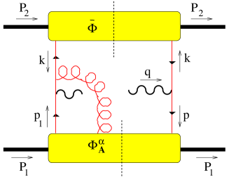
FIG. 1.: A diagram contributing to the Drell-Yan process at order $1/Q$.

The diagrams with first of all zero or one $A^{+}$ gluon(s) that we need to consider are (schematically) displayed in Fig. 2. We have only drawn the relevant left part of the diagrams and left out the blobs denoting the correlation functions, so gluons going to the bottom (top) emanate from $\Phi$ ($\overline{\Phi}$). For instance, Fig. 2b represents Fig. 1. The index $\alpha$ in Fig. 2b can be either transverse ($T$) or $+$ and it turns out that $\alpha$ and $\beta$ in Fig. 2c will be $T$ and $+$ respectively, otherwise the diagram will give a suppressed contribution; on the other diagrams we have indicated the appropriate gluon polarization (collinear or transverse).

The diagrams (h) and (i) are the only diagrams with a triple gluon vertex, since others will either be of higher order in $\alpha_{s}$ or cannot be separated from the soft part, since not all momenta are participating in the hard scattering and soft momentum loops will appear. We will first ignore the issue of color matrices in the diagrams without a triple gluon vertex and return to this point after we have considered the diagrams (a)-(g), i.e., after Eq. (59).

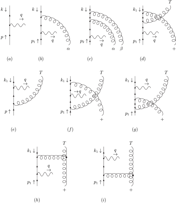
FIG. 2.: A subset of diagrams to be considered upon inclusion of zero or one $A^{+}$ gluon(s).

To discuss the expressions for the diagrams as given in the figure, we will introduce the shorthand notation:

$$\Big{[}\!\!\Big{[}\,\ldots\,\Big{]}\!\!\Big{]}\equiv\int d^{4}k\,d^{4}p\,\delta^{4}(p+k-q)\,{\text{Tr}}\left[\ldots\right]$$ (34)

Also, we need the precise definitions of $\Phi_{A}^{\alpha}(p_{1},p)$ and $\Phi_{AA}^{\alpha\beta}(p_{2},p_{1},p)$ ($\alpha,\beta$ not restricted to be transverse) and the antiquark correlation functions $\overline{\Phi}(k),\overline{\Phi}_{A}^{\alpha}(k_{1},k)$:

$$\Phi_{A}^{\alpha}(p_{1},p) = \int\frac{d^{4}x}{(2\pi)^{4}}\,\frac{d^{4}y}{(2\pi)^{4}}\ e^{ip\cdot y}\,e^{ip_{1}\cdot(x-y)}\,\langle P_{1},S_{1}|\overline{\psi}(0)\,gA^{\alpha}(y)\,\psi(x)|P_{1},S_{1}\rangle,$$ (35)

$$\Phi_{AA}^{\alpha\beta}(p_{2},p_{1},p) = \int\frac{d^{4}x}{(2\pi)^{4}}\,\frac{d^{4}y}{(2\pi)^{4}}\,\frac{d^{4}z}{(2\pi)^{4}}\ e^{ip\cdot z}\,e^{ip_{1}\cdot(y-z)}\,e^{ip_{2}\cdot(x-y)}\,\langle P_{1},S_{1}|\overline{\psi}(0)\,gA^{\beta}(z)\,gA^{\alpha}(y)\,\psi(x)|P_{1},S_{1}\rangle,$$ (36)

$$\overline{\Phi}(k) = \int\frac{d^{4}x}{(2\pi)^{4}}\,e^{-i\,k\cdot x}\langle P_{2},S_{2}|\psi(x)\overline{\psi}(0)|P_{2},S_{2}\rangle,$$ (37)

$$\overline{\Phi}_{A}^{\alpha}(k_{1},k) = \int\frac{d^{4}x}{(2\pi)^{4}}\,\frac{d^{4}y}{(2\pi)^{4}}\,e^{-i\,k\cdot(x-y)}e^{-i\,k_{1}\cdot y}\langle P_{2},S_{2}|\psi(x)gA^{\alpha}(y)\overline{\psi}(0)|P_{2},S_{2}\rangle.$$ (38)

The hadron momenta $P_{1},P_{2}$ (chosen such that $P_{1}\cdot P_{2}={\cal O}(Q^{2})$) and photon momentum $q$ are decomposed as

$$P_{1}^{\mu}\equiv\frac{Q}{x\sqrt{2}}\,n_{+}^{\mu}+\frac{xM_{1}^{2}}{Q\sqrt{2}}\,n_{-}^{\mu},$$ (39)

$$P_{2}^{\mu}\equiv\frac{\bar{x}M_{2}^{2}}{Q\sqrt{2}}\,n_{+}^{\mu}+\frac{Q}{\bar{x}\sqrt{2}}\,n_{-}^{\mu},$$ (40)

$$q^{\mu}\equiv\frac{Q}{\sqrt{2}}\,n_{+}^{\mu}+\frac{Q}{\sqrt{2}}\,n_{-}^{\mu}+q_{T}^{\mu},$$ (41)

for $Q_{T}^{2}\equiv-q_{T}^{2}\ll Q^{2}$. Furthermore, we decompose the parton momenta as ($i=1,2,\ldots$)

$$p\equiv\frac{Q}{\sqrt{2}}\,n_{+}+\frac{(p^{2}+\mathchoice{{\hbox{\boldmath$\displaystyle p$}}}{{\hbox{\boldmath$\textstyle p$}}}{{\hbox{\boldmath$\scriptstyle p$}}}{{\hbox{\boldmath$\scriptscriptstyle p$}}}_{T}^{2})}{Q\sqrt{2}}\,n_{-}+p_{T},$$ (42)

$$p_{i}\equiv\frac{\xi_{i}Q}{\sqrt{2}}\,n_{+}+\frac{(p_{i}^{2}+\mathchoice{{\hbox{\boldmath$\displaystyle p$}}}{{\hbox{\boldmath$\textstyle p$}}}{{\hbox{\boldmath$\scriptstyle p$}}}{{\hbox{\boldmath$\scriptscriptstyle p$}}}_{iT}^{2})}{\xi_{i}Q\sqrt{2}}\,n_{-}+p_{iT},$$ (43)

$$k\equiv\frac{Q}{\sqrt{2}}\,n_{-}+\frac{(k^{2}+\mathchoice{{\hbox{\boldmath$\displaystyle k$}}}{{\hbox{\boldmath$\textstyle k$}}}{{\hbox{\boldmath$\scriptstyle k$}}}{{\hbox{\boldmath$\scriptscriptstyle k$}}}_{T}^{2})}{Q\sqrt{2}}\,n_{+}+k_{T},$$ (44)

$$k_{i}\equiv\frac{\bar{\xi}_{i}Q}{\sqrt{2}}\,n_{-}+\frac{(k_{i}^{2}+\mathchoice{{\hbox{\boldmath$\displaystyle k$}}}{{\hbox{\boldmath$\textstyle k$}}}{{\hbox{\boldmath$\scriptstyle k$}}}{{\hbox{\boldmath$\scriptscriptstyle k$}}}_{iT}^{2})}{\bar{\xi}_{i}Q\sqrt{2}}\,n_{+}+k_{iT}.$$ (45)

We find for diagrams (a)-(d):

$$(a) = \Big{[}\!\!\Big{[}\Phi(p)\gamma^{\mu}\overline{\Phi}(k)\gamma^{\nu}\Big{]}\!\!\Big{]},$$ (46)

$$(b) = \Big{[}\!\!\Big{[}\Phi_{A}^{\alpha}(p)\gamma^{\mu}\overline{\Phi}(k)\gamma_{\alpha T}\frac{\mbox{$\not\!n_{+}$}}{\sqrt{2}Q}\gamma^{\nu}\Big{]}\!\!\Big{]}+\Big{[}\!\!\Big{[}\int d^{4}p_{1}\,\Phi_{A}^{+}(p_{1},p)\,\frac{\sqrt{2}}{Q(1-\xi_{1}+i\epsilon)}\,\gamma^{\mu}\overline{\Phi}(k)\gamma^{\nu}\Big{]}\!\!\Big{]}$$ (47)

$$+ \Big{[}\!\!\Big{[}\int d^{4}p_{1}\,\Phi_{A}^{+}(p_{1},p)\gamma^{\mu}\overline{\Phi}(k)\frac{\sqrt{2}}{Q(1-\xi_{1}+i\epsilon)}\left\{\frac{\mbox{$\not\!n_{+}$}}{\sqrt{2}Q}\left(\mbox{$\not\!k_{T}$}+\mbox{$\not\!p_{T}$}-\mbox{$\not\!p_{1T}$}\right)-P_{-}\right\}\gamma^{\nu}\Big{]}\!\!\Big{]},$$ (48)

$$(c) = \Big{[}\!\!\Big{[}\int d^{4}p_{2}\,d^{4}p_{1}\,\Phi_{AA}^{\alpha\,+}(p_{2},p_{1},p)\,\frac{\sqrt{2}}{Q(1-\xi_{1}+i\epsilon)}\,\gamma^{\mu}\overline{\Phi}(k)\gamma_{\alpha T}\frac{\mbox{$\not\!n_{+}$}}{\sqrt{2}Q}\gamma^{\nu}\Big{]}\!\!\Big{]},$$ (49)

$$(d) = \Big{[}\!\!\Big{[}\int d^{4}p_{1}\,\Phi_{A}^{+}(p_{1},p)\gamma^{\mu}\left(\int d^{4}k_{1}\,\overline{\Phi}_{D}^{\beta}(k_{1},k)\gamma_{\beta T}+\overline{\Phi}(k)\mbox{$\not\!k_{T}$}\right)\frac{\sqrt{2}}{Q(1-\xi_{1}+i\epsilon)}\frac{\mbox{$\not\!n_{+}$}}{\sqrt{2}Q}\gamma^{\nu}\Big{]}\!\!\Big{]}.$$ (50)

In the last equation we have used the fact that in the $A^{-}=0$ gauge no link operator will be present in $\overline{\Phi}_{A}^{\beta}$. We can then apply the equations of motion to $\int d^{4}k_{1}\,\overline{\Phi}_{D}^{\beta}(k_{1},k)\gamma_{\beta T}$, which results (in the $A^{-}=0$ gauge) in a cancellation of the term with the $P_{-}=\mbox{$\not\!n_{-}$}\mbox{$\not\!n_{+}$}/2$ projector in the expression for diagram (b). Anticipating the specific link operators that will result in the end, we observe that

$$\Phi[-\infty,x](p) \equiv \int\frac{d^{4}x}{(2\pi)^{4}}\,e^{ip\cdot x}\,\langle P_{1},S_{1}|\overline{\psi}(0)\,{\cal L}^{+}[-\infty,x]\,\psi(x)|P_{1},S_{1}\rangle$$ (51)

$$= \Phi(p)+\int d^{4}p_{1}\,\Phi_{A}^{+}(p_{1},p)\frac{\sqrt{2}}{Q(1-\xi_{1}+i\epsilon)}+\ldots,$$ (52)

$$\Phi_{A}^{\alpha}[-\infty,x](p) \equiv \int\frac{d^{4}x}{(2\pi)^{4}}\,e^{ip\cdot x}\,\langle P_{1},S_{1}|\overline{\psi}(0)\,{\cal L}^{+}[-\infty,x]\,gA^{\alpha}(x)\,\psi(x)|P_{1},S_{1}\rangle$$ (53)

$$= \Phi_{A}^{\alpha}(p)+\int d^{4}p_{2}\,d^{4}p_{1}\,\Phi_{AA}^{\alpha\,+}(p_{2},p_{1},p)\frac{\sqrt{2}}{Q(1-\xi_{1}+i\epsilon)}+\ldots,$$ (54)

where the definition of $\Phi_{A}^{\alpha}(p)$ is given in Eq. (33). The sum of the four diagrams (a)-(d) therefore results in (to order $g$ in the link operator)

$$(a)+(b)+(c)+(d) = \Big{[}\!\!\Big{[}\Phi[-\infty,x](p)\gamma^{\mu}\overline{\Phi}(k)\gamma^{\nu}\Big{]}\!\!\Big{]}+\Big{[}\!\!\Big{[}\Phi_{A}^{\alpha}[-\infty,x](p)\gamma^{\mu}\overline{\Phi}(k)\gamma_{\alpha T}\frac{\mbox{$\not\!n_{+}$}}{\sqrt{2}Q}\gamma^{\nu}\Big{]}\!\!\Big{]}$$ (55)

$$+ \Big{[}\!\!\Big{[}\int d^{4}p_{1}\,\Phi_{A}^{+}(p_{1},p)\gamma^{\mu}\overline{\Phi}(k)\frac{\sqrt{2}}{Q(1-\xi_{1}+i\epsilon)}\frac{\mbox{$\not\!n_{+}$}}{\sqrt{2}Q}\left(\mbox{$\not\!p_{T}$}-\mbox{$\not\!p_{1T}$}\right)\gamma^{\nu}\Big{]}\!\!\Big{]}.$$ (56)

By taking into account the derivative of the link operator, the last two terms nicely combine into the following expression containing exclusively the functions $\Phi[-\infty,x](p)$ and $\Phi_{D}^{\alpha}[-\infty,x](p)$ (the latter is obtained from Eq. (54) by replacing $gA^{\alpha}$ by $iD^{\alpha}$):

$$(a)+(b)+(c)+(d) = \Big{[}\!\!\Big{[}\Phi[-\infty,x](p)\gamma^{\mu}\overline{\Phi}(k)\gamma^{\nu}\Big{]}\!\!\Big{]}$$ (57)

$$+ \Big{[}\!\!\Big{[}\left\{\Phi_{D}^{\alpha}[-\infty,x](p)-p^{\alpha}\,\Phi[-\infty,x](p)\right\}\gamma^{\mu}\overline{\Phi}(k)\gamma_{\alpha T}\frac{\mbox{$\not\!n_{+}$}}{\sqrt{2}Q}\gamma^{\nu}\Big{]}\!\!\Big{]}.$$ (58)

The diagrams (e)-(g) also turn out to combine, yielding the (expected) expression:

$$(e)+(f)+(g)=-\Big{[}\!\!\Big{[}\Phi[-\infty,x](p)\gamma^{\mu}\left\{\gamma_{0}\overline{\Phi}_{D}^{\beta\dagger}(k)\gamma_{0}+k^{\beta}\overline{\Phi}(k)\right\}\gamma^{\nu}\frac{\mbox{$\not\!n_{-}$}}{\sqrt{2}Q}\gamma_{\beta T}\Big{]}\!\!\Big{]},$$ (59)

where we used that $\int d^{4}k_{1}\overline{\Phi}_{D}^{\beta}(k_{1},k)=\gamma_{0}\overline{\Phi}_{D}^{\beta\dagger}(k)\gamma_{0}$, when $\overline{\Phi}_{D}^{\beta}(k)\equiv\int d^{4}k_{1}\overline{\Phi}_{D}^{\beta}(k,k_{1})$, cf. Ref. [19]. To arrive at Eq. (59) we also made use of the fact that to this order $\overline{\Phi}_{A}^{\alpha}$ (with $\alpha$ transverse) will be proportional to $\not\!n_{-}$ and that $\Phi_{A}^{+}$ will be proportional to $\not\!n_{+}$.

Until now we have ignored the issue of color matrices. It is easy to see that in diagrams (d), (f) and (g) the color matrices are in the wrong order for them to be absorbed into the correlation functions along with the link operators. The diagrams with the triple gluon vertex should be included to cancel the contributions arising from commuting the two color matrices. In this way diagram (h) will cancel the term arising from diagram (d) and diagram (i) that of diagrams (f) and (g). Hence, by including diagram (h) and (i) one can include the color matrices in the link operators.

This concludes the case of including zero or one $A^{+}$ gluon(s) (emanating from $\Phi$, connecting to the left). Inclusion of two $A^{+}$ gluons is done in a similar fashion, where we note that from diagram (c) with $\alpha=\beta=+$ one can see that a product of two theta-functions in the minus component appears, which gives rise to the path-ordering. Knowing this, it is a matter of iteratively treating each order like the first order we have discussed just now, by considering $\left\{\Phi_{D}^{\alpha}[-\infty,x](p)-p^{\alpha}\,\Phi[-\infty,x](p)\right\}$ as an effective $\Phi_{A}^{\alpha}(p)$.

When the $A^{+}$ gluons emanating from $\Phi$ connect to the right side of the diagrams, then one arrives at the link operator

$${\cal L}^{+}[0,-\infty]=\left.{\cal P}\exp\left(ig\int_{-\infty}^{0^{-}}dy^{-}\,A^{+}(y)\right)\right|_{y^{+}=0^{+},\mathchoice{{\hbox{\boldmath$\displaystyle y$}}}{{\hbox{\boldmath$\textstyle y$}}}{{\hbox{\boldmath$\scriptstyle y$}}}{{\hbox{\boldmath$\scriptscriptstyle y$}}}_{T}=\mathchoice{{\hbox{\boldmath$\displaystyle 0$}}}{{\hbox{\boldmath$\textstyle 0$}}}{{\hbox{\boldmath$\scriptstyle 0$}}}{{\hbox{\boldmath$\scriptscriptstyle 0$}}}_{T}}.$$ (60)

Inclusion of arbitrary numbers of $A^{+}$ gluons emanating from $\Phi$ connecting to either side of the diagram, results in the appearance of the following color gauge invariant correlation functions exclusively:

$$\Phi_{\text{GI}}(p) \equiv \int\frac{d^{4}x}{(2\pi)^{4}}\,e^{ip\cdot x}\,\langle P_{1},S_{1}|\overline{\psi}(0)\,{\cal L}^{+}[0,-\infty]\,{\cal L}^{+}[-\infty,x]\,\psi(x)|P_{1},S_{1}\rangle,$$ (61)

$$\Phi_{D\,\text{GI}}^{\alpha}(p_{1},p) \equiv \int\frac{d^{4}x}{(2\pi)^{4}}\,\frac{d^{4}y}{(2\pi)^{4}}\ e^{ip\cdot y}\,e^{ip_{1}\cdot(x-y)}\,\langle P_{1},S_{1}|\overline{\psi}(0)\,{\cal L}^{+}[0,-\infty]$$ (63)

$$\times\,{\cal L}^{+}[-\infty,y]\,iD^{\alpha}(y)\,{\cal L}^{+}[y,-\infty]\,{\cal L}^{+}[-\infty,x]\,\psi(x)|P_{1},S_{1}\rangle.$$

Hence, Eqs. (61) and (63) are the Drell-Yan process extentions of Eqs. (10) and (11) to the case the correlation functions not only depend on the lightcone momentum fractions.

So we conclude that at the tree level the complete set of diagrams with arbitrary numbers of $A^{+}$ gluons emanating from $\Phi$ will result in the appearance of color gauge invariant correlation functions (containing link operators and covariant derivatives), with path-ordered exponentials having paths along lightlike directions extending to lightcone infinity. Not choosing the $A^{-}=0$ gauge cannot affect $\Phi_{\text{GI}}$ or $\Phi_{D\,\text{GI}}^{\alpha}$ to this order ($1/Q$) and hence, these are the correlation functions that will appear in any gauge. Choosing the $A^{+}=0$ gauge instead, will give rise to similar results for $\overline{\Phi}$ and $\overline{\Phi}_{D}^{\alpha}$. The color gauge invariant matrix elements $\overline{\Phi}_{\text{GI}}(k)$ and $\overline{\Phi}_{D\,\text{GI}}^{\alpha}(k_{1},k)$ contain similar links extending to lightcone infinity, but now involving $A^{-}$ gluon fields:

$$\overline{\Phi}_{\text{GI}}(k) \equiv \int\frac{d^{4}x}{(2\pi)^{4}}\,e^{-i\,k\cdot x}\langle P_{2},S_{2}|\psi(x)\,{\cal L}^{-}[x,-\infty]\,{\cal L}^{-}[-\infty,0]\,\overline{\psi}(0)|P_{2},S_{2}\rangle,$$ (64)

$$\overline{\Phi}_{D\,\text{GI}}^{\alpha}(k_{1},k) \equiv \int\frac{d^{4}x}{(2\pi)^{4}}\,\frac{d^{4}y}{(2\pi)^{4}}\,e^{-i\,k\cdot(x-y)}e^{-i\,k_{1}\cdot y}\langle P_{2},S_{2}|\psi(x)\,{\cal L}^{-}[x,-\infty]$$ (66)

$$\times\,{\cal L}^{-}[-\infty,y]\,iD^{\alpha}(y)\,{\cal L}^{-}[y,-\infty]\,{\cal L}^{-}[-\infty,0]\,\overline{\psi}(0)|P_{2},S_{2}\rangle,$$

where

$${\cal L}^{-}[x,-\infty]=\left.{\cal P}\exp\left(ig\int_{-\infty}^{x^{+}}dy^{+}\,A^{-}(y)\right)\right|_{y^{-}=x^{-},\mathchoice{{\hbox{\boldmath$\displaystyle y$}}}{{\hbox{\boldmath$\textstyle y$}}}{{\hbox{\boldmath$\scriptstyle y$}}}{{\hbox{\boldmath$\scriptscriptstyle y$}}}_{T}=\mathchoice{{\hbox{\boldmath$\displaystyle x$}}}{{\hbox{\boldmath$\textstyle x$}}}{{\hbox{\boldmath$\scriptstyle x$}}}{{\hbox{\boldmath$\scriptscriptstyle x$}}}_{T}}.$$ (67)

One thus finds the following color gauge invariant expression for the hadron tensor not integrated over the transverse momentum of the lepton pair, including $1/Q$ contributions:

$${\cal W}^{\mu\nu}(P_{1},P_{2},q) = \frac{1}{3}\,\int d^{4}k\,d^{4}p\,\delta^{4}(p+k-q)\,\Biggl{\{}{\text{Tr}}\left[\Phi_{\text{GI}}(p)\gamma^{\mu}\overline{\Phi}_{\text{GI}}(k)\gamma^{\nu}\right]$$ (68)

$$+ {\text{Tr}}\left[\left\{\int d^{4}p_{1}\,\Phi_{D\,\text{GI}}^{\alpha}(p_{1},p)-p^{\alpha}\,\Phi_{\text{GI}}(p)\right\}\gamma^{\mu}\overline{\Phi}_{\text{GI}}(k)\gamma_{\alpha T}\frac{\mbox{$\not\!n_{+}$}}{\sqrt{2}Q}\gamma^{\nu}\right]$$ (69)

$$- {\text{Tr}}\left[\Phi_{\text{GI}}(p)\gamma^{\mu}\left\{\int d^{4}k_{1}\,\overline{\Phi}_{D\,\text{GI}}^{\beta}(k_{1},k)+k^{\beta}\,\overline{\Phi}_{\text{GI}}(k)\right\}\gamma^{\nu}\frac{\mbox{$\not\!n_{-}$}}{\sqrt{2}Q}\gamma_{\beta T}\right]$$ (70)

$$+ {\text{Tr}}\left[\left\{\int d^{4}p_{1}\,\Phi_{D\,\text{GI}}^{\alpha}(p,p_{1})-p^{\alpha}\,\Phi_{\text{GI}}(p)\right\}\gamma^{\mu}\frac{\mbox{$\not\!n_{+}$}}{\sqrt{2}Q}\gamma_{\alpha T}\overline{\Phi}_{\text{GI}}(k)\gamma^{\nu}\right]$$ (71)

$$- {\text{Tr}}\left[\Phi_{\text{GI}}(p)\gamma_{\beta T}\frac{\mbox{$\not\!n_{-}$}}{\sqrt{2}Q}\gamma^{\mu}\left\{\int d^{4}k_{1}\,\overline{\Phi}_{D\,\text{GI}}^{\beta}(k,k_{1})+k^{\beta}\,\overline{\Phi}_{\text{GI}}(k)\right\}\gamma^{\nu}\right]\Biggl{\}}.$$ (72)

This expression still contains some order $1/Q^{2}$ contributions, which we ignore to keep the notation as simple as possible. To the order we consider one can for instance replace

$$\delta^{4}(p+k-q)\to\delta(q^{+}-p^{+})\,\delta(q^{-}-k^{-})\,\delta^{2}(\mathchoice{{\hbox{\boldmath$\displaystyle p$}}}{{\hbox{\boldmath$\textstyle p$}}}{{\hbox{\boldmath$\scriptstyle p$}}}{{\hbox{\boldmath$\scriptscriptstyle p$}}}_{T}+\mathchoice{{\hbox{\boldmath$\displaystyle k$}}}{{\hbox{\boldmath$\textstyle k$}}}{{\hbox{\boldmath$\scriptstyle k$}}}{{\hbox{\boldmath$\scriptscriptstyle k$}}}_{T}-\mathchoice{{\hbox{\boldmath$\displaystyle q$}}}{{\hbox{\boldmath$\textstyle q$}}}{{\hbox{\boldmath$\scriptstyle q$}}}{{\hbox{\boldmath$\scriptscriptstyle q$}}}_{T}).$$ (73)

To obtain the hadron tensor expression Eq. (72) we have already used these delta functions, for instance in the parametrizations of the momenta $q,p,k$.

We would like to emphasize that we have not obtained color gauge invariance at the cost of introducing a path dependence. The expansion in orders of $1/Q$ does not leave any freedom of choosing the paths for the leading and next-to-leading twist terms.

B Color gauge invariant correlation functions to all orders in $\alpha_{s}$

In order to extend the above tree level analysis to all orders in $\alpha_{s}$ in the hard scattering part, we will first discuss two limiting cases. The first case we consider is the cross section integrated over the transverse momentum $\mathchoice{{\hbox{\boldmath$\displaystyle q$}}}{{\hbox{\boldmath$\textstyle q$}}}{{\hbox{\boldmath$\scriptstyle q$}}}{{\hbox{\boldmath$\scriptscriptstyle q$}}}_{T}$ of the lepton pair. The second case is the cross section at measured $\mathchoice{{\hbox{\boldmath$\displaystyle q$}}}{{\hbox{\boldmath$\textstyle q$}}}{{\hbox{\boldmath$\scriptstyle q$}}}{{\hbox{\boldmath$\scriptscriptstyle q$}}}_{T}$ (with $\mathchoice{{\hbox{\boldmath$\displaystyle q$}}}{{\hbox{\boldmath$\textstyle q$}}}{{\hbox{\boldmath$\scriptstyle q$}}}{{\hbox{\boldmath$\scriptscriptstyle q$}}}_{T}^{2}\equiv Q_{T}^{2}\ll Q^{2}$), but restricted to the leading twist.

In case one integrates the cross section, and hence the hadron tensor, over the transverse momentum $\mathchoice{{\hbox{\boldmath$\displaystyle q$}}}{{\hbox{\boldmath$\textstyle q$}}}{{\hbox{\boldmath$\scriptstyle q$}}}{{\hbox{\boldmath$\scriptscriptstyle q$}}}_{T}$ of the lepton pair, then the situation simplifies considerably. After a collinear expansion of the hard scattering parts, the transverse momenta of the partons can be integrated over each separately. The hadron tensor will be expressed in terms of collinear partons only, i.e., they are collinear to the momentum direction of the parent hadron (neglecting target mass corrections). More specifically, the hadron tensor contains the above gauge invariant correlation functions $\Phi,\Phi_{D}^{\alpha}$ ($\overline{\Phi}$, $\overline{\Phi}_{D}^{\alpha}$) integrated over the $-$ ($+$) and transverse momentum components. They depend only on the lightcone momentum fractions, such as the ones that appear in the DIS cross section, cf. Eq. (10) and (11). In that case one can apply Ward identities to gluon fields with polarizations proportional to their momenta, to prove that the above results are also correct to all orders in $\alpha_{s}$ in the hard scattering part. This has been done for the leading twist contribution in for instance Refs. [12, 20], Ref. [17] (cf. its Fig. 4.4 and appendix) and Ref. [14] (cf. its Figs. 19 and 25 and Eqs. (131) and (133)). It is completely analogous to the application of Eq. (19) in DIS. Also, it straightforwardly applies to the $1/Q$ corrections for which a factorization theorem has been discussed in Ref. [21]. The same Ward identities can be applied, since the additional $A_{T}$ gluon has physical polarization and is on-shell and therefore, does not affect how the collinear gluons appear in the Ward identities. The latter just produce link operators on both side of the $A_{T}$ field and since in this case the links are independent of transverse coordinates, the replacement $gA_{T}\to iD_{T}-i\partial_{T}$ immediately gives the result for $\int d^{2}\mathchoice{{\hbox{\boldmath$\displaystyle q$}}}{{\hbox{\boldmath$\textstyle q$}}}{{\hbox{\boldmath$\scriptstyle q$}}}{{\hbox{\boldmath$\scriptscriptstyle q$}}}_{T}\,{\cal W}^{\mu\nu}(P_{1},P_{2},q)$, using ${\cal W}^{\mu\nu}$ from Eq. (72) with hard scattering parts $H$ containing all orders in $\alpha_{s}$:

$$\int d^{2}\mathchoice{{\hbox{\boldmath$\displaystyle q$}}}{{\hbox{\boldmath$\textstyle q$}}}{{\hbox{\boldmath$\scriptstyle q$}}}{{\hbox{\boldmath$\scriptscriptstyle q$}}}_{T}\,{\cal W}^{\mu\nu}(x,\bar{x},\mathchoice{{\hbox{\boldmath$\displaystyle q$}}}{{\hbox{\boldmath$\textstyle q$}}}{{\hbox{\boldmath$\scriptstyle q$}}}{{\hbox{\boldmath$\scriptscriptstyle q$}}}_{T})=\frac{1}{3}\,\Biggl{\{}\text{Tr}\left[\Phi_{\text{GI}}(x)\overline{\Phi}_{\text{GI}}(\bar{x})H^{\mu\nu}(x,\bar{x})\right]$$ (74)

$$\quad+\text{Tr}\left[\int\,dy\,\left\{\Phi_{D\,\text{GI}}^{\alpha}(y,x)-\delta(y-x)\int\,d^{4}p\,\delta(p^{+}-xP_{1}^{+})\,p^{\alpha}\,\Phi_{\text{GI}}(p)\right\}\overline{\Phi}_{\text{GI}}(\bar{x})\,H_{1\,\alpha}^{\mu\nu}(y,x,\bar{x})\right]$$ (75)

$$\quad+\text{Tr}\left[\Phi_{\text{GI}}(x)\,\int\,d\bar{y}\,\left\{\overline{\Phi}_{D\,\text{GI}}^{\alpha}(\bar{y},\bar{x})+\delta(\bar{y}-\bar{x})\int\,d^{4}k\,\delta(k^{-}-\bar{x}P_{2}^{-})\,k^{\alpha}\overline{\Phi}_{\text{GI}}(k)\right\}H_{2\,\alpha}^{\mu\nu}(x,\bar{y},\bar{x})\right]\Biggr{\}}.$$ (76)

This is just a schematic way of writing, since the four spinor indices on the hard scattering part $H^{\mu\nu}$ and $H_{\alpha}^{\mu\nu}$ connects to both $\Phi$ and $\overline{\Phi}$. At tree level this equation is Eq. (27) re-expressed in terms of color gauge invariant functions, Eqs. (10), (11) and the obvious extensions $\overline{\Phi}_{\text{GI}}(\bar{x})$ and $\overline{\Phi}_{D\,\text{GI}}^{\alpha}(\bar{x},\bar{y})$. This holds in case soft gluon poles are assumed to be absent. Our previous tree level analysis is in this case an explicit demonstration of a result valid to all orders in $\alpha_{s}$, since soft gluons can be shown to cancel [21].

To apply such Ward identities to the more extended case we considered here, namely to the cross section differential in the transverse momentum $\mathchoice{{\hbox{\boldmath$\displaystyle q$}}}{{\hbox{\boldmath$\textstyle q$}}}{{\hbox{\boldmath$\scriptstyle q$}}}{{\hbox{\boldmath$\scriptscriptstyle q$}}}_{T}$ of the lepton pair ($Q_{T}^{2}\ll Q^{2}$), is more complicated. The momenta of the partons are in general not collinear to the parent hadron, since they also possess some transverse momentum. Hence, the $A^{+}$ gluons, i.e., the gluons that are collinear to the parent hadron do not have polarization collinear to their own momenta. The latter type of gluons are called gluons with longitudinal polarization [14] and are the gluons to which Ward identities can be applied directly. For the leading twist contribution the application of such Ward identities still works for $A^{+}$ gluons, because deviations of $A^{+}$ gluons from longitudinal polarization (such deviations are proportional to $A_{T}$) will be suppressed by inverse powers of the hard scale. We then find for the leading twist part of Eq. (72) with a hard part $H$ containing all orders in $\alpha_{s}$:

$${\cal W}^{\mu\nu}(x,\bar{x},\mathchoice{{\hbox{\boldmath$\displaystyle q$}}}{{\hbox{\boldmath$\textstyle q$}}}{{\hbox{\boldmath$\scriptstyle q$}}}{{\hbox{\boldmath$\scriptscriptstyle q$}}}_{T})=\frac{1}{3}\int\,d^{2}\mathchoice{{\hbox{\boldmath$\displaystyle p$}}}{{\hbox{\boldmath$\textstyle p$}}}{{\hbox{\boldmath$\scriptstyle p$}}}{{\hbox{\boldmath$\scriptscriptstyle p$}}}_{T}\,d^{2}\mathchoice{{\hbox{\boldmath$\displaystyle k$}}}{{\hbox{\boldmath$\textstyle k$}}}{{\hbox{\boldmath$\scriptstyle k$}}}{{\hbox{\boldmath$\scriptscriptstyle k$}}}_{T}\,\delta^{2}(\mathchoice{{\hbox{\boldmath$\displaystyle p$}}}{{\hbox{\boldmath$\textstyle p$}}}{{\hbox{\boldmath$\scriptstyle p$}}}{{\hbox{\boldmath$\scriptscriptstyle p$}}}_{T}+\mathchoice{{\hbox{\boldmath$\displaystyle k$}}}{{\hbox{\boldmath$\textstyle k$}}}{{\hbox{\boldmath$\scriptstyle k$}}}{{\hbox{\boldmath$\scriptscriptstyle k$}}}_{T}-\mathchoice{{\hbox{\boldmath$\displaystyle q$}}}{{\hbox{\boldmath$\textstyle q$}}}{{\hbox{\boldmath$\scriptstyle q$}}}{{\hbox{\boldmath$\scriptscriptstyle q$}}}_{T})\,{\text{Tr}}\left[\Phi_{\text{GI}}(x,\mathchoice{{\hbox{\boldmath$\displaystyle p$}}}{{\hbox{\boldmath$\textstyle p$}}}{{\hbox{\boldmath$\scriptstyle p$}}}{{\hbox{\boldmath$\scriptscriptstyle p$}}}_{T})\,\overline{\Phi}_{\text{GI}}(\bar{x},\mathchoice{{\hbox{\boldmath$\displaystyle k$}}}{{\hbox{\boldmath$\textstyle k$}}}{{\hbox{\boldmath$\scriptstyle k$}}}{{\hbox{\boldmath$\scriptscriptstyle k$}}}_{T})\,H^{\mu\nu}(x,\bar{x},\mathchoice{{\hbox{\boldmath$\displaystyle p$}}}{{\hbox{\boldmath$\textstyle p$}}}{{\hbox{\boldmath$\scriptstyle p$}}}{{\hbox{\boldmath$\scriptscriptstyle p$}}}_{T},\mathchoice{{\hbox{\boldmath$\displaystyle k$}}}{{\hbox{\boldmath$\textstyle k$}}}{{\hbox{\boldmath$\scriptstyle k$}}}{{\hbox{\boldmath$\scriptscriptstyle k$}}}_{T},\mathchoice{{\hbox{\boldmath$\displaystyle q$}}}{{\hbox{\boldmath$\textstyle q$}}}{{\hbox{\boldmath$\scriptstyle q$}}}{{\hbox{\boldmath$\scriptscriptstyle q$}}}_{T})\right].$$ (77)

However, this is not the complete result, since if one goes beyond the tree level, then apart from having a more complicated hard scattering part, soft gluons have to be resummed into Sudakov form factors [4], resulting in a replacement

$$\delta^{2}(\mathchoice{{\hbox{\boldmath$\displaystyle p$}}}{{\hbox{\boldmath$\textstyle p$}}}{{\hbox{\boldmath$\scriptstyle p$}}}{{\hbox{\boldmath$\scriptscriptstyle p$}}}_{T}+\mathchoice{{\hbox{\boldmath$\displaystyle k$}}}{{\hbox{\boldmath$\textstyle k$}}}{{\hbox{\boldmath$\scriptstyle k$}}}{{\hbox{\boldmath$\scriptscriptstyle k$}}}_{T}-\mathchoice{{\hbox{\boldmath$\displaystyle q$}}}{{\hbox{\boldmath$\textstyle q$}}}{{\hbox{\boldmath$\scriptstyle q$}}}{{\hbox{\boldmath$\scriptscriptstyle q$}}}_{T})\to\int\frac{d^{2}\mathchoice{{\hbox{\boldmath$\displaystyle b$}}}{{\hbox{\boldmath$\textstyle b$}}}{{\hbox{\boldmath$\scriptstyle b$}}}{{\hbox{\boldmath$\scriptscriptstyle b$}}}}{(2\pi)^{2}}\,e^{-i\mathchoice{{\hbox{\boldmath$\displaystyle b$}}}{{\hbox{\boldmath$\textstyle b$}}}{{\hbox{\boldmath$\scriptstyle b$}}}{{\hbox{\boldmath$\scriptscriptstyle b$}}}\cdot(\mathchoice{{\hbox{\boldmath$\displaystyle p$}}}{{\hbox{\boldmath$\textstyle p$}}}{{\hbox{\boldmath$\scriptstyle p$}}}{{\hbox{\boldmath$\scriptscriptstyle p$}}}_{T}+\mathchoice{{\hbox{\boldmath$\displaystyle k$}}}{{\hbox{\boldmath$\textstyle k$}}}{{\hbox{\boldmath$\scriptstyle k$}}}{{\hbox{\boldmath$\scriptscriptstyle k$}}}_{T}-\mathchoice{{\hbox{\boldmath$\displaystyle q$}}}{{\hbox{\boldmath$\textstyle q$}}}{{\hbox{\boldmath$\scriptstyle q$}}}{{\hbox{\boldmath$\scriptscriptstyle q$}}}_{T})}\,e^{-S(\mathchoice{{\hbox{\boldmath$\displaystyle b$}}}{{\hbox{\boldmath$\textstyle b$}}}{{\hbox{\boldmath$\scriptstyle b$}}}{{\hbox{\boldmath$\scriptscriptstyle b$}}})},$$ (78)

where $e^{-S(\mathchoice{{\hbox{\boldmath$\displaystyle b$}}}{{\hbox{\boldmath$\textstyle b$}}}{{\hbox{\boldmath$\scriptstyle b$}}}{{\hbox{\boldmath$\scriptscriptstyle b$}}})}$ is the Sudakov form factor. This has been shown in Ref. [3, 18] for the leading twist.

For the next-to-leading twist a factorization proof for the cross section differential in the transverse momentum of the lepton pair ($Q_{T}^{2}\ll Q^{2}$) has not been given. But we will discuss how Ward identities applied to longitudinally polarized gluons can be used to show that collinear gluons factorize, i.e., they exponentiate into link operators, also at next-to-leading twist (${\cal O}(1/Q)$).

From our tree level result we can deduce how the deviations of longitudinally polarized gluons from collinearity will affect the application of the Ward identities. The part of a longitudinally polarized gluon field $A_{\text{lp}}^{\mu}\sim p^{\mu}$ that deviates from the $n_{+}$ direction (i.e., from its $A^{+}$ part) will be proportional to its transverse momentum ($A_{\text{lp}\,T}^{\mu}\sim p_{T}^{\mu}$). The latter part will generate derivatives of the $A^{+}$ parts of the other additional longitudinally polarized gluons, which to this order can be taken to be collinear. This yields the derivative of a link operator that is exactly needed to compensate for the effect of the replacement $gA\to iD-i\partial$ inside $\Phi_{A}^{\alpha}$ (which now contains link operators depending on transverse coordinates), in order to arrive at the replacement $\Phi_{A}^{\alpha}(p)\to\Phi_{D}^{\alpha}(p)-p^{\alpha}\Phi(p)$ for correlation functions containing link operators. At tree level this is the step from Eq. (56) to Eq. (58).

To make this a bit more explicit we write down the longitudinally polarized gluon field in Fig. 1:

$$A_{\text{lp}}^{\alpha}=n_{+}^{\alpha}(n_{-}\cdot A)+\left(p_{T}^{\alpha}-p_{1T}^{\alpha}\right)\frac{\sqrt{2}}{Q(1-\xi_{1}+i\epsilon)}(n_{-}\cdot A)\,\propto\,(p^{\alpha}-p_{1}^{\alpha}).$$ (79)

Insertion of this field into the most general hard part (Fig. 1 contains only the tree level hard part) and applying the Ward identity will result in those diagrams where the longitudinally polarized gluon attaches directly to the “external” legs of the hard part (those legs that connect to the soft parts), cf. Ref. [14]. The $A^{+}$ part of $A_{\text{lp}}^{\alpha}$ will yield a term in a link operator in $\Phi$ (represented by a double line in Ref. [14], called an eikonal line) and the second term on the r.h.s. of Eq. (79) will give rise to the derivative of a link operator in $\Phi_{A}^{\alpha}$. At tree level these are the first and third term of Eq. (56), respectively.

It is easy to verify that this will work to all orders in $\alpha_{s}$ in the hard part, since one has to take this deviation into account for only one longitudinally polarized gluon. Hence, our conclusion is that transverse momentum dependence in correlation functions does not spoil the summation of collinear $A^{+}$ gluons into link operators at next-to-leading twist (${\cal O}(1/Q)$). This is not in conflict with the known failure of factorization at even higher twist [22].

Hence, Eq. (72) can then be written with a hard part $H$ containing all orders in $\alpha_{s}$:

$${\cal W}^{\mu\nu}(P_{1},P_{2},q) = \frac{1}{3}\,\int d^{4}k\,d^{4}p\,\delta^{4}(p+k-q)\,\Biggl{\{}{\text{Tr}}\left[\Phi_{\text{GI}}(p)\,\overline{\Phi}_{\text{GI}}(k)\,H^{\mu\nu}(p,k,q)\right]$$ (80)

$$+ {\text{Tr}}\left[\int d^{4}p_{1}\,\left\{\Phi_{D\,\text{GI}}^{\alpha}(p_{1},p)-\delta(p_{1}-p)\,p^{\alpha}\,\Phi_{\text{GI}}(p)\right\}\,\overline{\Phi}_{\text{GI}}(k)\,H_{1\,\alpha}^{\mu\nu}(p,k,q)\right]$$ (81)

$$+ {\text{Tr}}\left[\Phi_{\text{GI}}(p)\,\int d^{4}k_{1}\,\left\{\overline{\Phi}_{D\,\text{GI}}^{\beta}(k_{1},k)+\delta(k_{1}-k)\,k^{\beta}\,\overline{\Phi}_{\text{GI}}(k)\right\}\,H_{2\,\beta}^{\mu\nu}(p,k,q)\right]\Biggl{\}}.$$ (82)

Again soft gluons will have to be included and they will modify the delta function.

Application of Ward identities are an essential part of the proof of factorization. They are used to show that collinear gluons exponentiate, like discussed above, but also that soft gluons factorize from the hard part and from the correlation functions. In the $\mathchoice{{\hbox{\boldmath$\displaystyle q$}}}{{\hbox{\boldmath$\textstyle q$}}}{{\hbox{\boldmath$\scriptstyle q$}}}{{\hbox{\boldmath$\scriptscriptstyle q$}}}_{T}$-integrated case the soft gluons must be shown to cancel and in the case of measured $\mathchoice{{\hbox{\boldmath$\displaystyle q$}}}{{\hbox{\boldmath$\textstyle q$}}}{{\hbox{\boldmath$\scriptstyle q$}}}{{\hbox{\boldmath$\scriptscriptstyle q$}}}_{T}$ they must be shown to exponentiate into Sudakov factors. For the next-to-leading twist the latter case has not been studied yet, but the application of collinear Ward identities as discussed above will be an essential ingredient. The fact that Ward identities can be used to show that collinear gluons also exponentiate at next-to-leading twist in the case of measured $\mathchoice{{\hbox{\boldmath$\displaystyle q$}}}{{\hbox{\boldmath$\textstyle q$}}}{{\hbox{\boldmath$\scriptstyle q$}}}{{\hbox{\boldmath$\scriptscriptstyle q$}}}_{T}$ (with $Q_{T}^{2}\ll Q^{2}$), suggests that collinear Ward identities can also be applied to the soft gluon exponentiation and a factorization theorem is expected to hold. It could of course be the case that the replacement Eq. (78) is different for these subleading terms than for the leading term. This has to be investigated further.

Finally, we have to remark that additional divergences are introduced by the paths extending to infinity if one considers $\alpha_{s}$ corrections connecting to the paths; these have to be renormalized. A discussion on this topic and how to deal with it is given in [3] and applies unchanged to the next-to-leading twist results discussed here.

C Color gauge invariant soft gluon poles

Until now we have considered the case where we assume all fields at infinity to vanish inside the hadronic matrix elements. In the case of soft gluon poles this assumption is relaxed in a specific way. To include such contributions one has to make the following replacement (cf. Eq. (27)) in the first term in Eq. (48) for diagram (b) and in Eq. (49) for diagram (c):

$$\frac{\mbox{$\not\!n_{+}$}}{\sqrt{2}Q}\to\frac{\mbox{$\not\!n_{+}$}}{\sqrt{2}Q}\frac{1-\xi_{1}}{1-\xi_{1}+i\epsilon}.$$ (83)

A soft gluon pole means that the correlation function has a pole at $\xi_{1}=1$, i.e., when the gluon has vanishing momentum. This prohibits applying the inverse of the above replacement [2].

If we consider the above replacement the following matrix element (times $\delta(p^{+}-p_{1}^{+})$) results (in addition to the matrix elements in Eq. (72)):

$$\int\frac{d^{4}x}{(2\pi)^{4}}\,\frac{d^{4}y}{(2\pi)^{4}}\ e^{ip\cdot y}\,e^{ip_{1}\cdot(x-y)}\,\langle P_{1},S_{1}|\overline{\psi}(0)\,{\cal L}^{+}[0,-\infty]$$ (85)

$$\qquad\qquad\qquad\times\frac{1}{2}\frac{\partial}{\partial y^{-}}\left({\cal L}^{+}[-\infty,y]\,gA_{T}^{\alpha}(y)\,{\cal L}^{+}[y,-\infty]\right)\,{\cal L}^{+}[-\infty,x]\,\psi(x)|P_{1},S_{1}\rangle.$$

Due to time reversal symmetry and under the assumption of continuity of the correlation functions, one can show [2] that for soft gluon poles one has to have antisymmetric boundary conditions on the field $A_{T}$ at $y^{-}=\pm\infty$. In this case one can replace $gA_{T}\to iD_{T}$ in the above matrix element. The identity

$$\left[\frac{\partial}{\partial y^{-}},{\cal L}^{+}[-\infty,y]\,iD^{\alpha}(y)\,{\cal L}^{+}[y,-\infty]\right]={\cal L}^{+}[-\infty,y]\,gF^{+\alpha}(y)\,{\cal L}^{+}[y,-\infty]$$ (86)

is used to arrive from Eq. (85) at

$$\Phi_{F\,\text{GI}}^{\alpha}(p_{1},p) \equiv \int\frac{d^{4}x}{(2\pi)^{4}}\,\frac{d^{4}y}{(2\pi)^{4}}\ e^{ip\cdot y}\,e^{ip_{1}\cdot(x-y)}\,\langle P_{1},S_{1}|\overline{\psi}(0)\,{\cal L}^{+}[0,-\infty]$$ (88)

$$\times\,{\cal L}^{+}[-\infty,y]\,\frac{g}{2}F^{+\alpha}(y)\,{\cal L}^{+}[y,-\infty]\,{\cal L}^{+}[-\infty,x]\,\psi(x)|P_{1},S_{1}\rangle,$$

where $\alpha$ is transverse. The gauge invariant term $\Phi_{F\,\text{GI}}^{\alpha}(p_{1},p)$ will show up in the hadron tensor Eq. (72) in exactly the same way as $\Phi_{D\,\text{GI}}^{\alpha}(p_{1},p)$. In Eq. (72) one can just replace

$$\Phi_{D\,\text{GI}}^{\alpha}(p_{1},p)\to\Phi_{D\,\text{GI}}^{\alpha}(p_{1},p)+\Phi_{F\,\text{GI}}^{\alpha}(p_{1},p)\,\delta(p^{+}-p_{1}^{+}).$$ (89)

We find that upon choosing the $A^{+}=0$ gauge in $\int d^{4}p_{1}d^{4}p\,\Phi_{F\,\text{GI}}^{\alpha}(p_{1},p)\delta(p^{+}-p_{1}^{+})$ that the standard expression for the soft gluon pole matrix element $T(x,S_{T})$ as given in [6, 2] results, cf. Eqs. (3) and (5) (note that we have now included a factor $g/2$ in the matrix element $\Phi_{F\,\text{GI}}^{\alpha}$).

From the above it is clear that soft gluon poles require nonzero matrix elements containing $A_{T}$ fields at $y^{-}=\pm\infty$ in any gauge. On the other hand, we have chosen hadronic matrix elements with $A^{+}$ fields at $y^{-}=\pm\infty$ to vanish. The reason is that otherwise the previously obtained matrix elements will not be color gauge invariant anymore and their derivation will not even be well-defined, i.e., will not result in finite answers, since

$$\int dp_{1}^{+}\Phi_{A}^{+}(p_{1},p)\frac{\sqrt{2}}{Q(1-\xi_{1}+i\epsilon)}$$ (90)

will be divergent. We simply conclude that soft gluon poles arise from gluon fields with physical (transverse) polarizations.

Hence, the inclusion of soft gluon poles can be done in a color gauge invariant way, even in the case where the transverse momentum of the lepton pair is not integrated over.

As a final point we note that in the color gauge invariant correlation functions $\Phi_{D\,\text{GI}}^{\alpha}$ and $\Phi_{F\,\text{GI}}^{\alpha}$ the index $\alpha$ is purely transverse, reflected in the appearance of $\gamma_{T}^{\alpha}$ in Eq. (72) (analogous to the projector $\omega$ in DIS). Imposing the additional, but unnecessary constraint of $n_{-}$-independence at this stage will alter the expression for the hadron tensor and may result in different answers.

V Conclusions

We have considered the color gauge invariance of a factorized description of the Drell-Yan process cross section. The analysis focused on next-to-leading twist contributions for polarized scattering (${\cal O}(1/Q)$) and on the cross section differential in the transverse momentum of the lepton pair ($Q_{T}^{2}\ll Q^{2}$). The hadron tensor has been expressed in terms of manifestly color gauge invariant, nonlocal operator matrix elements. The tree level case was worked out explicitly and Ward identities, applied to longitudinally polarized gluons, allowed to extend the results to all orders in the hard scattering part. This use of Ward identities in case longitudinally polarized gluons are not equal to collinear gluons will also be an important ingredient in a full (and still lacking) factorization proof for the case under consideration, to be given in a gauge independent way. The factorization, i.e., exponentiation into Sudakov factors, of soft gluons is expected to be analogous to the factorization and exponentiation of collinear gluons as derived here.

The leading twist part of the expressions we have derived, are in agreement with earlier investigations [3, 18]. Moreover, the whole result (including the next-to-leading twist) reduces to known results [21] upon integration over the transverse momentum of the lepton pair. We have also given a color gauge invariant treatment of soft gluon poles, showing that in any gauge such poles arise from gluon fields with physical (transverse) polarizations. In addition, we have extensively discussed the discrepancy between the results of Ref. [1] and [2] for a single transverse spin asymmetry in the Drell-Yan process. This asymmetry appears at the tree level in case soft gluon poles in the twist-three matrix elements are present. We have demonstrated that the requirement of $n_{-}$-independence of the resulting factorized hadron tensor expression as imposed in Refs. [1, 11] is unnecessary from the point of Lorentz and gauge invariance and leads to a different answer in the case of the above mentioned asymmetry. Without imposing this requirement the derivative term will not be present in the asymmetry expression at tree level. We have carefully considered the color gauge invariance of the description of the cross section in terms of the matrix elements, to conclude that only physical, i.e., transverse gluon degrees of freedom contribute and hence, arrive at the expression $A_{2}$ (Eq. (2) or equivalently Eq. (8)) for the asymmetry.

REFERENCES

• [1] N. Hammon, O. Teryaev and A. Schäfer, Phys. Lett. B 390 (1997) 409.
• [2] D. Boer, P.J. Mulders and O.V. Teryaev, Phys. Rev. D 57 (1998) 3057.
• [3] J.C. Collins, D.E. Soper and G. Sterman, Phys. Lett. B 109 (1982) 388; Nucl. Phys. B 223 (1983) 381; Phys. Lett. B 126 (1983) 275.
• [4] J.C. Collins, in Perturbative Quantum Chromodynamics, Ed. A.H. Mueller (World Scientific, Singapore, 1989), p. 573.
• [5] I.I. Balitsky and V.M. Braun, Nucl. Phys. B 361 (1991) 93.
• [6] J. Qiu and G. Sterman, Phys. Rev. Lett. 67 (1991) 2264; Nucl. Phys. B 378 (1992) 52.
• [7] V.M. Korotkiyan and O.V. Teryaev, Dubna preprint E2-94-200; Phys. Rev. D 52 (1995) R4775.
• [8] A.V. Efremov, V.M. Korotkiyan and O.V. Teryaev, Phys. Lett. B 384 (1995) 577.
• [9] J. Qiu and G. Sterman, Phys. Rev. D 59 (1999) 014004.
• [10] R.K. Ellis, W. Furmanski and R. Petronzio, Nucl. Phys. B 212 (1983) 29; Nucl. Phys. B 207 (1982) 1.
• [11] A.V. Efremov and O.V. Teryaev, Sov. J. Nucl. Phys. 39 (1984) 962.
• [12] A.V. Efremov and A.V. Radyushkin, Theor. Math. Phys. 44 (1981) 774.
• [13] J.C. Collins and D.E. Soper, Nucl. Phys. B 194 (1982) 445.
• [14] J.C. Collins, D.E. Soper and G. Sterman, in Perturbative Quantum Chromodynamics, Ed. A.H. Mueller (World Scientific, Singapore, 1989), p. 1.
• [15] J. Qiu and G. Sterman, Nucl. Phys. B 353 (1991) 105; Nucl. Phys. B 353 (1991) 137.
• [16] R.L. Jaffe and X. Ji, Phys. Rev. Lett. 67 (1991) 552; Nucl. Phys. B 375 (1992) 527.
• [17] J.C. Collins, D.E. Soper and G. Sterman, Nucl. Phys. B 261 (1985) 104.
• [18] J.C. Collins, D.E. Soper and G. Sterman, Nucl. Phys. B 250 (1985) 199; G.T. Bodwin, Phys. Rev. D 31 (1985) 2616; Phys. Rev. D 34 (1986) 3932 (E).
• [19] P.J. Mulders and R.D. Tangerman, Nucl. Phys. B 461 (1996) 197; Nucl. Phys. B 484 (1997) 538 (E).
• [20] R.K. Ellis, H. Georgi, M. Machacek, H.D. Politzer and G.G. Ross, Nucl. Phys. B 152 (1979) 285.
• [21] J. Qiu and G. Sterman, Proceedings of the Polarized Collider Workshop, Eds. J.C. Collins, S.F. Heppelman and R.W. Robinett, University Park, PA (1990), AIP Conf. Proc. No. 223, (AI, New York, 1990), p. 249.
• [22] R. Doria, J. Frenkel and J.C. Taylor, Nucl. Phys. B 168 (1980) 93;
C. Di’Lieto, S. Gendron, I.G. Halliday and C.T. Sachrajda, Nucl. Phys. B 183 (1981) 223;
R. Basu, A.J. Ramalho and G. Sterman, Nucl. Phys. B 244 (1984) 221
F.T. Brandt, J. Frenkel and J.C. Taylor, Nucl. Phys. B 312 (1989) 589.