Feynman-Schwinger representation approach to nonperturbative physics

Abstract

The Feynman-Schwinger representation provides a convenient framework for the calculation of nonperturbative propagators. In this paper we first investigate an analytically solvable case, namely the scalar QED in 0+1 dimension. With this toy model we illustrate how the formalism works. The analytic result for the self energy is compared with the perturbative result. Next, using a $\chi^{2}\phi$ interaction, we discuss the regularization of various divergences encountered in this formalism. The ultraviolet divergence, which is common in standard perturbative field theory applications, is removed by using a Pauli-Villars regularization. We show that the divergence associated with large values of Feynman-Schwinger parameter $s$ is spurious and it can be avoided by using an imaginary Feynman parameter $is$.

I Introduction

In nuclear physics one is often faced by problems that require nonperturbative methods. The best known example is the problem of bound states. Even if the underlying theory may have a small coupling constant (such as in QED), and therefore allows the use of perturbation theory in general, the treatment of bound states are inherently nonperturbative. The n-body bound state is defined by the pole of the interacting n-body propagator. A perturbative approximation of n-body propagator does not produce the bound state pole location. This can most easily be seen by the following example:

$$\frac{1}{1-x}=1+x+x^{2}+x^{3}+\,.\,.\,.$$ (1)

Any truncation of the righthandside (perturbation theory) will fail to produce the pole which is located at $x=1$. Therefore it is essential that reliable nonperturbative methods that take all orders of interaction into account are developed. For this reason, numerous nonperturbative methods have been developed and succesfully used in the literature. Some of the best known examples are relativistic bound state equations [1, 2, 3], and lattice gauge theory [4].

Relativistic bound state equations provide a practical and intuitive framework to analyze bound states. However this practicality comes with certain drawbacks. In particular, the bound state equations in general lack gauge invariance. The second problem is associated with the fact that a completely self consistent solution of bound state equations is very difficult. A completely self consistent solution requires solving infinitely many coupled equations for all n-point functions of the theory. Since this is an impossible task, one is either forced to model various vertices and interaction kernels or specify them perturbatively.

The second and more recent approach is known as lattice gauge theory (LGT). LGT is a Euclidean path integral based approach which relies on the discretization of space-time. An economical lattice simulation with a small lattice size of $5^{4}$ requires roughly $4\,({\rm links})\times 8\,({\rm real\,\,SU(3)\,\,parameters})\times 5^{4}\,({\rm space-timepoints})=20000$ integrations. In general with larger lattice sizes this cost goes as $32N^{4}$. The disadvantage of discretization is twofold. The first one is the excessive computational time required for lattice simulations. The second problem is the anomalies caused by the discretization, such as the fermion doubling problem [4].

In this paper we discuss yet another method known as the Feynman-Schwinger Representation (FSR)  [5, 6, 7]. Similar to the LGT, the FSR approach is also based on Euclidean path integral formalism. The basic idea in the FSR approach is to integrate out all fields at the expense of introducing quantum mechanical path integrals over the trajectories of particles. Replacing the path integrals over fields with path integrals over trajectories has an enormous computational advantage. In the FSR approach, a calculation similar to the example given above requires only $4N$ integrations, where $N$ is now the steps a particle takes between the initial and final states. In addition to this enormous savings in computational time, the FSR approach also employs a space time continuum and therefore does not suffer from problems such as fermion doubling and the continuum limit.

An additional motivation in studying the FSR approach is to determine which subsets of diagrams give the dominant contribution to the n-body propagator. This is particularly important in determining what kind of approximations are reasonable within the context of bound state equations. Therefore the FSR is a very promising tool to do this. In this paper we report on results for the 2-point function. In studies of hadronic systems like $\pi N$ one usually models the self-energy contribution through the lowest order one-loop graph. Also this is used as a starting point for the improved action procedure proposed by Lepage [8]. It is clearly useful to compare such a lowest order approximation with the full results obtained from a FSR calculation. We study here as a toy model the scalar QED (SQED) in 0 space and 1 time dimension, which can be solved analytically. The intriguing issue we also address in this paper is the difficulty found in the Euclidean action functional for the case of a $\phi^{3}$-theory. In applying the FSR to the 4-point function in the case of a $\phi^{3}$-theory confined to generalized ladders one encounters a difficulty that the Euclidean action diverges. It was conjectured and demonstrated in a simple example by Nieuwenhuis [9] that this problem arises due to the continuation to the Euclidean metric. This problem is examined in detail here and we in particular show that there exists a regularization method to remove this divergence. As a result a clear prescription is given for dealing in a proper way with the Euclidean action in this case.

The organization of this paper is as follows: In the next section we start by discussing the case of SQED in 0+1 dimension. This is a simple case which can be worked out analytically. We consider the one-body and two-body propagators. We compare the one-body result for the dressed mass with the perturbation theory result. In the third section we consider the case of scalar interaction $\chi^{2}\phi$ in 3+1 dimension. We consider the issue of Wick rotation in Feynman parameter $s$, and present the FSR result for the one-body dressed mass obtained by Monte-Carlo integration. The result is again compared by the perturbation theory prediction.

II Scalar QED

Massive scalar QED in 0+1 dimension is a simple interaction that enables one to obtain a fully analytical result for the dressed and bound state masses within the FSR approach. In this section we compare the self energy result obtained by perturbative methods with the full result obtained from the Feynman-Schwinger representation. The Minkowski metric expression for the scalar QED Lagrangian in Stueckelberg form is given by

$${\cal L}_{SQED}=-m^{2}\chi^{2}-\frac{1}{4}F^{2}+\frac{1}{2}\mu^{2}A^{2}-\lambda\frac{1}{2}(\partial A)^{2}+(\partial_{\mu}-ieA_{\mu})\chi^{*}(\partial^{\mu}+ieA^{\mu})\chi,$$ (2)

where $A$ represents the gauge field of mass $\mu$, and $\chi$ is the charged field of mass $m$. We employ the Feynman gauge ($\lambda=1$). The presence of a mass term for the exchange field breaks the gauge invariance. Here the mass term was introduced in order to avoid infrared singularities which are present in 0+1 dimension. For dimensions larger than n=2 the infrared singularity does not exist and therefore the limit $\mu\rightarrow$ can be safely taken to restore the gauge invariance. Since we confine ourselves to 0+1 dimension, the antisymmetric tensor $F^{\mu\nu}$ vanishes. Therefore, in Euclidean metric and in 0+1 dimension, the scalar QED Lagrangian can be written as

$${\cal L}_{SQED}^{E}=\biggl{[}m^{2}\chi^{2}+(\partial\chi)^{2}+\frac{1}{2}\,\mu^{2}A^{2}+\frac{1}{2}\,(\partial A)^{2}+e^{2}\chi^{2}A^{2}-ieA(\chi^{*}\partial\chi-\chi\partial\chi^{*})\biggr{]}.$$ (3)

In preparation for the path integration which will be performed below, it is more convenient to cast the Lagrangian into the following form

$${\cal L}_{SQED}^{E}=\chi^{*}\biggl{[}m^{2}-\partial^{2}-2ieA\partial-ie\partial A+e^{2}A^{2}\biggr{]}\chi+\frac{1}{2}A(\mu^{2}-\partial^{2})A.$$ (4)

In order to construct a gauge invariant Green’s function G, we introduce a gauge link $U(x,y)$

$$U(x,y)\equiv{\rm exp}\left[-ie\int_{x}^{y}dz\,A(z)\right].$$ (5)

The two-body Green’s function for the transition from the initial state $\Phi_{i}=\chi^{*}(x)U(x,\bar{x})\chi(\bar{x})$ to final state $\Phi_{f}=\chi^{*}(y)U^{*}(y,\bar{y})\chi(\bar{y})$ is given by

$$G(y,\bar{y}|x,\bar{x})=N\int{\cal D}\chi^{*}\int{\cal D}\chi\int{\cal D}A\,\,\Phi^{*}_{f}\Phi_{i}\,e^{-S_{E}},$$ (6)

where

$$S_{E}=\int d^{4}x\,\,{\cal L}_{SQED}^{E}.$$ (7)

Performing the path integrals over $\chi$ and $\chi^{*}$ fields one finds

$$G(y,\bar{y}|x,\bar{x}) = N\int{\cal D}A\,({\rm det}S)^{-1}U(x,\bar{x})U^{*}(y,\bar{y})\left[S(x,y)S(\bar{x},\bar{y})+S(x,\bar{x})S(y,\bar{y})\right]$$ (9)

$$\,\,\,\,\,\,\,\,\,\,\,\,\,\,\,\,\,\,\,\,\times\,{\rm exp}\left[-\frac{1}{2}\int d^{4}zA(z)(\mu^{2}-\partial^{2})A(z)\right],$$

where the interacting propagator is defined by

$$S(x,y)\equiv<y\,|\,\frac{1}{m^{2}-\partial^{2}-2ieA\,\partial-ie\partial A+e^{2}A^{2}}\,|\,x>.$$ (10)

As in lattice gauge theory calculations we use the quenched approximation, ${\rm det}S\rightarrow 1$. In order to be able to carry out the remaining path integral over the exchange field $A$ it is desirable to represent the interacting propagator in the form of an exponential. This can be achieved by using a Feynman representation for the interacting propagator.

$$S(x,y)=<y\,|\int_{0}^{-i\infty}ds\,\,{\rm exp}\biggl{[}-s(m^{2}-\partial^{2}-2ieA\,\partial-ie\partial A+e^{2}A^{2}+i\epsilon)\biggr{]}|\,x>,$$ (11)

where the $s$ integration is along the imaginary axis. Let us now define

$$U(x,y,s)\equiv<y\,|\,{\rm exp}\biggl{[}-s(-\partial^{2}-2ieA\,\partial-ie\partial A+e^{2}A^{2})\biggr{]}|\,x>$$ (12)

where $U(x,y,s)$ satisfies

$$\frac{\partial}{\partial s}U(x,y,s)=(\partial^{2}+2ieA\,\partial+ie\partial A-e^{2}A^{2})U(x,y,s).$$ (13)

This is equivalent to the Schroedinger equation for imaginary time $t=is$, with Hamiltonian

$$H(p,z)=(p+ieA(z))^{2}.$$ (14)

The matrix element of the interacting propagator Eq. (11) can be written in terms of a quantum mechanical path integral. We know from quantum mechanics that

$$<y\,|\,{\rm exp}[-iH(q,p)\,t]\,|\,x>=\int{\cal D}q\,{\rm exp}\biggl{[}\,i\int_{0}^{\infty}{\cal L}(q(t),\dot{q}(t))\,dt\,\biggr{]}.$$ (15)

The Lagrangian for Eq. (14) is given by

$$L(z,\dot{z})=\frac{\dot{z}^{2}}{4}-ie\dot{z}A(z).$$ (16)

Therefore, the quantum mechanical path integral representation for this propagator is given by

$$S(x,y)=-i\int_{0}^{\infty}ds\int{\cal D}z\,{\rm exp}\biggl{[}is(m^{2}+i\epsilon)-i/4\int_{0}^{s}d\tau\,\dot{z}^{2}(\tau)+ie\int_{0}^{s}d\tau\,\dot{z}A(z(\tau))\biggr{]},$$ (17)

where the boundary conditions are given by $z(0)=x$, $z(s)=y$. This representation allows one to perform the remaining path integral over the exchange field $A$. The final result for the two-body propagator involves a quantum mechanical path integral that sums up contributions coming from all possible trajectories of particles

$$G=-\int_{0}^{\infty}ds\int_{0}^{\infty}d\bar{s}\int({\cal D}z)_{xy}\int({\cal D}\bar{z})_{\bar{x}\bar{y}}\,e^{-S[Z]},$$ (18)

where $S[Z]$ is given by

$$S[Z]\equiv-iK[z,s]-iK[\bar{z},\bar{s}]+V[z,\bar{z}].$$ (19)

The free and the interaction contributions to $S[Z]$ are given as

$$K[z,s] = (m^{2}+i\epsilon)s-\frac{1}{4s}\int_{0}^{1}d\tau\,\frac{dz_{\mu}(\tau)}{d\tau}\frac{dz^{\mu}(\tau)}{d\tau},$$ (20)

$$V[z,\bar{z}] = +\frac{e^{2}}{2}\oint_{C}d\tau\,\dot{z}(\tau)\oint_{C}d\bar{\tau}\,\dot{\bar{z}}(\bar{\tau})\,\Delta(z(\tau)-\bar{z}(\bar{\tau}),\mu),$$ (21)

$$\Delta(x,\mu) = \int\frac{dp}{2\pi}\frac{e^{ipx}}{p^{2}+\mu^{2}}=\frac{e^{-\mu|z|}}{2\mu},$$ (22)

where $\Delta(x)$ is the interaction kernel. $K[z,s]$ represents the mass term and the kinetic term, and $V[z,s]$ includes the self energy and the exchange interaction contributions (shown in Fig. 1). The contour of integration $C$ follows a counterclockwise trajectory $x\rightarrow y\rightarrow\bar{y}\rightarrow\bar{x}\rightarrow x$ as parameters $\tau$, and $\bar{\tau}$ are varied from 0 to $1$. The self energy and the exchange interaction contributions, which are embedded in expression 21, have different signs. This follows from the fact that particles forming the two body bound state carry opposite charges.

FIG. 1.: A sample trajectory of each particle along with various interactions are shown.

The bound state spectrum can be determined from the spectral decomposition of the two body Green’s function

$$G(T)=\sum_{n=0}^{\infty}c_{n}e^{-m_{n}T},$$ (23)

where T is defined as the average time between the initial and final states

$$T\equiv\frac{1}{2}(y_{4}+\bar{y}_{4}-x_{4}-\bar{x}_{4}).$$ (24)

In the limit of large $T$, the ground state mass is given by

$$m_{0}=\lim_{T\rightarrow\infty}-\frac{d}{dT}ln[G(T)]=\frac{\int{\cal D}ZS^{\prime}[Z]e^{-S[Z]}}{\int{\cal D}Ze^{-S[Z]}},$$ (25)

A The one-body case

In order to be able to compare with the perturbative result later, we concentrate on the one-body case. The one-body propagator is given by

$$G(0,T)=\int ds\int({\cal D}z)_{0T}\,{\rm exp}\biggl{[}iK[z,s]-V_{0}[z]\biggr{]}.$$ (26)

The integral of the self interaction Eq. (21) can analytically be performed

$$V_{0}[z] = \frac{e^{2}}{4\mu}\int_{0}^{1}d\tau\,\dot{z}(\tau)\int_{0}^{1}d\bar{\tau}\,\dot{z}(\bar{\tau})\,e^{-\mu|z(\tau)-z(\bar{\tau})|},$$ (27)

$$= \frac{e^{2}T}{2\mu^{2}}\biggl{[}1-\frac{1-e^{-\mu T}}{\mu T}\biggr{]},$$ (28)

where the boundary conditions were chosen as $z(0)=0$, and $z(1)=T$. Next, the path integral over $z$ can be evaluated after a discretization in proper time. Since the only path dependence in the propagator is in the kinetic term, the path integral over $z$ involves gaussian integrals which can be performed easily by using the following discretization

$$({\cal D})_{0T}\rightarrow(N/4\pi s)^{N/2}\Pi^{N-1}_{i=1}\int dz_{i}.$$ (29)

The $s$ integral can also be evaluated by saddle point method giving

$$G(0,T)=N{\rm exp}\biggl{[}-mT-e^{2}\frac{T}{2\mu^{2}}+\frac{e^{2}}{2\mu^{3}}(1-e^{-\mu T})\biggr{]}.$$ (30)

This is an exact result for large times $T$. The dressed mass can easily be obtained by taking the logarithmic derivative of this expression. Therefore, the one-body dressed mass for SQED in 0+1 dimension according to the FSR formalism is given by

$$M=m+\frac{e^{2}}{2\mu^{2}}.$$ (31)

Simplicity of the SQED in 0+1 dimension also allows one to get an analytical result for the two-body bound state mass. It can easily be seen that the two-body result for the total mass is given by

$$M_{bound}=\left(m+\frac{e^{2}}{2\mu^{2}}\right)+\left(m+\frac{e^{2}}{2\mu^{2}}\right)-\frac{e^{2}}{\mu^{2}}=2m,$$ (32)

where the first two terms are due to the one-body contributions and the last term is due to the exchange interaction. The exchange contribution to the mass (up to a missing factor of two), was also reported earlier in Ref. [9]. The interesting feature of the result in Eq. (32) is the fact that the positive shift of one-body masses are exactly compensated by the negative binding energy created by the exchange interaction. Therefore the total bound state mass is exactly equal to the sum of bare masses. Therefore in this simple case vertex corrections do not contribute to the bound state mass.

In order to be able to compare with the FSR prediction Eq. (31) we consider the perturbative treatment of self energy.

B The perturbative result

In this section we consider the perturbative treatment of the self energy and compare the perturbative result with the FSR prediction Eq. (31). The self energy (Figure 2) in 0+1 dimension is given by

$$\Sigma(p)=-ie^{2}\int_{-\infty}^{\infty}\frac{dk}{2\pi}\frac{(2p-k)^{2}}{(k^{2}-\mu^{2})[(p-k)^{2}-m^{2}]}+ie^{2}\int_{\infty}^{\infty}\frac{dk}{2\pi}\frac{1}{k^{2}-\mu^{2}}.$$ (33)

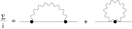
FIG. 2.: Self energy for the SQED.

Performing the Wick rotation we get the following Euclidean expression

$$\Sigma(p)=-e^{2}\int_{-\infty}^{\infty}\frac{dk}{2\pi}\biggl{[}\frac{(2p-k)^{2}}{(k^{2}+\mu^{2})[(p-k)^{2}+m^{2}]}-\frac{1}{k^{2}+\mu^{2}}\biggr{]}.$$ (34)

Evaluating the integral we find

$$\Sigma(p)=-\frac{e^{2}}{2}\biggl{[}\frac{(i\mu-2p)^{2}}{\mu[m^{2}+(i\mu-p)^{2}]}+\frac{(im-p)^{2}}{m[\mu^{2}+(im+p)^{2}]}-\frac{1}{\mu}\biggr{]}.$$ (35)

The dressed propagator corresponding to this self energy is

$$-i\Delta_{d}(p)= \frac{-i}{m^{2}+p^{2}}+\frac{-i}{m^{2}+p^{2}}\biggl{\{}-i\Sigma_{E}(p)\biggr{\}}\frac{-i}{m^{2}+p^{2}}+\cdots$$ (36)

$$= \frac{-i}{m^{2}+p^{2}+\Sigma_{E}(p)}\,.$$ (37)

The coordinate space form of the dressed propagator is

$$\Delta_{d}(t)=\int_{-\infty}^{\infty}\frac{dp}{2\pi}\left(\frac{e^{ipt}}{m^{2}+p^{2}+\Sigma_{E}(p)}\right)\simeq Ne^{-Mt}\,.$$ (38)

where $M$ is the dressed mass and $N$ is a normalization factor. The dependence of $M$ on the coupling strength $e$ can be obtained from the solution of the on-shell condition

$$M=\sqrt{m^{2}+\Sigma_{E}(iM)},$$ (39)

which must be real if the dressed mass is to be stable. Therefore, for SQED, the equation determining the dressed mass takes the following form

$$M^{2}=m^{2}+\frac{e^{2}}{2}\biggl{[}\frac{(\mu-2M)^{2}}{\mu[m^{2}-(\mu-M)^{2}]}+\frac{(m-M)^{2}}{m[\mu^{2}-(m+M)^{2}]}+\frac{1}{\mu}\biggr{]}.$$ (40)

This perturbative result can be compared with the exact result Eq. (31) found earlier. In figure 3 we present the case of $m=\mu=1$ GeV. For small values of coupling strength $e^{2}$ the perturbative and the full results converge. From the figure we see, that although the higher loop contributions cannot entirely be neglected they are of limited size, suggesting that in this case the lowest one-loop contribution may be a reasonable approximation for not too strong couplings. This is consistent with the results from Ref. [9] in the case of SQED in 2+1 dimension. The perturbative result develops a complex mass beyond a critical coupling $e^{2}_{crit}=0.343$ (GeV)². At the critical point a ’collision’ takes place with another real solution of Eq. (40), leading to two complex conjugated solutions with increasing $e^{2}$. This happens at $M=1.49$ GeV. This is an inadequacy of the perturbative approach.

The occurrence of complex ghost poles in the propagator has also been found in Lee-like models [10, 11] and in $\pi-N$-interaction models [12]. Moreover, it is also interesting to note that a similar critical behaviour was also observed within the context of one body Dyson-Schwinger equation in Ref. [13]. In the Dyson-Schwinger-Bethe-Salpeter studies of hadron structure the lack of real and finite mass poles in the quark propagator is usually considered as an indication of confinement. On the other hand, the simple example of SQED study in 0+1 dimension shows that while the exact result for the dressed mass obtained from the FSR approach produces a real mass pole for all values of the coupling, the simple bubble sumation leads to complex mass poles for large coupling values. Therefore the connection between confinement and lack of real mass poles is far from clear.

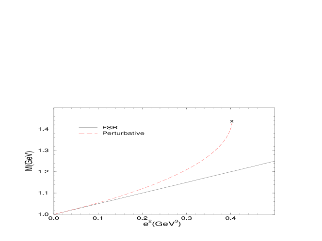
FIG. 3.: The function $M(g^{2})$ calculated by the FSR approach and the perturbative methods for values of $m=\mu=1$ GeV. According to the perturbative result there is a critical point at $g^{2}_{crit}=0.343$ (GeV)² beyond which the dressed mass becomes complex.

Having presented the study of SQED in 0+1 dimension, where analytical results are easily obtained and compared with the perturbative ones, we move on to the scalar $\chi^{2}\phi$ interaction in 3+1 dimension.

III The Feynman-Schwinger formalism for scalar fields

We consider the theory of charged scalar particles $\chi$ of mass $m$ interacting through the exchange of a neutral scalar particle $\phi$ of mass $\mu$. For this case the analytical integration of path integrals are not possible and one needs computational tools.

The Euclidean Lagrangian for this theory is given by

$${\cal L}_{E}=\chi^{*}\bigl{[}m^{2}-\partial^{2}+g\phi\bigr{]}\chi+\frac{1}{2}\,\phi(\mu^{2}-\partial^{2})\phi.$$ (41)

The two body Green’s function for the transition from the initial state $\Phi_{i}=\chi^{*}(x)\chi(\bar{x})$ to final state $\Phi_{f}=\chi^{*}(y)\chi(\bar{y})$ is given by

$$G(y,\bar{y}|x,\bar{x})=N\int{\cal D}\chi^{*}\int{\cal D}\chi\int{\cal D}\phi\,\Phi^{*}_{f}\Phi_{i}\,e^{-S_{E}}.$$ (42)

Performing the path integrals over $\chi$ and $\chi^{*}$ fields one finds

$$G(y,\bar{y}|x,\bar{x})=N\int{\cal D}\phi\,({\rm det}S)^{-1}[S(x,y)S(\bar{x},\bar{y})+S(x,\bar{x})S(y,\bar{y})]e^{-\frac{1}{2}\int d^{4}z\phi(\mu^{2}-\partial^{2})\phi},$$ (43)

where the interacting propagator is defined by

$$S(x,y)\equiv<y\,|\,\frac{1}{m^{2}-\partial^{2}+g\phi}\,|\,x>.$$ (44)

In order to be able to carry out the remaining path integral over the exchange field $\phi$ it is desirable to represent the interacting propagator in the form of an exponential.

$$S(x,y)=<y\,|\int_{0}^{-i\infty}ds\,e^{-s(m^{2}-\partial^{2}+g\phi+i\epsilon)}|\,x>.$$ (45)

Here we want to comment on a subtlety about the Feynman representation. In earlier works[5, 6] the following Feynman representation was used

$$S(x,y)\equiv<y\,|\int_{0}^{\infty}ds\,e^{-s(m^{2}-\partial^{2}+g\phi)}|\,x>,\\$$ (46)

The validity of this representation depends on the sign of the field $\phi$ which can be either positive or negative. If one accepts this representation, the problem manifests itself as an exponentially diverging $s$ dependence after the path integral over $\phi$ is performed. In order to circumvent the problem of the $s$ singularity we use the Feynman representation given in Eq. (45). Let us define

$$U(x,y,s)\equiv<y\,|e^{-s(-\partial^{2}+g\phi)}|\,x>,$$ (47)

where $U(x,y,s)$ satisfies

$$\frac{\partial}{\partial s}U(x,y,s)=(\partial^{2}-g\phi)U(x,y,s).$$ (48)

This is equivalent to the Schroedinger equation for imaginary time $t=is$, with Hamiltonian

$$H(p,z)=p^{2}-g\phi(z).$$ (49)

The Lagrangian for the Hamiltonian given in Eq. (49) is

$$L(z,\dot{z})=\frac{\dot{z}^{2}}{4}+g\phi(z).$$ (50)

Therefore, the interacting propagator can be expressed as

$$S(x,y)=-i\int_{0}^{\infty}ds\int{\cal D}z\,{\rm exp}\biggl{[}is(m^{2}+i\epsilon)-i/4\int_{0}^{s}d\tau\,\dot{z}^{2}(\tau)+ig\int_{0}^{s}d\tau\,\phi(z(\tau))\biggr{]},$$ (51)

where the boundary conditions are given by $z(0)=x$, $z(s)=y$. The final result for the two-body propagator involves a quantum mechanical path integral that sums up contributions coming from all possible trajectories of particles. The only difference from the SQED case Eq. (17) is the replacement of $e\dot{z}A(z(\tau))\rightarrow g\phi$. Therefore, for the two body propagator one arrives at the same expresion as Eq. (18) except now the new definition (compare with Eq. (21)) of the interaction term is

$$V[z,\bar{z},s,\bar{s}] = V_{0}[z,s]+2V_{12}[z,\bar{z},s,\bar{s}]+V_{0}[\bar{z},\bar{s}],$$ (52)

where

$$V_{0}[z,s] = \frac{g^{2}}{2}s^{2}\int_{0}^{1}d\tau\int_{0}^{1}d\tau^{\prime}\,\Delta(z(\tau)-z(\tau^{\prime}),\mu),$$ (53)

$$V_{12}[z,\bar{z},s,\bar{s}] = \frac{g^{2}}{2}s\bar{s}\int_{0}^{1}d\tau\int_{0}^{1}d\bar{\tau}\,\Delta(z(\tau)-\bar{z}(\bar{\tau}),\mu).$$ (54)

Here the $V_{0}[z,s]$ term represents the self energy contribution, while the $V_{12}[z,\bar{z},s,\bar{s}]$ term represents the exchange interaction (Fig. 1). The notable difference compared to the SQED case is that the interaction terms now depend on the $s$ variable. The second difference from the SQED case is the fact that self energy and exchange interaction terms have the same signs. The interaction kernel $\Delta(x)$ is defined by

$$\Delta(x,\mu) = \int\frac{d^{4}p}{(2\pi)^{4}}\frac{e^{ip\cdot x}}{p^{2}+\mu^{2}}=\frac{\mu}{4\pi^{2}|x|}K_{1}(\mu|x|).$$ (55)

The time of propagation, T, is defined as before in Eq. (24)

In principle one can work with equation (25), using the interaction given in Eq. (52), to determine the ground state energy of the bound state. However this is in practice very costly. The problem is the oscillatory behavior of the integrand which forbids the use of Monte-Carlo techniques for integration. Therefore it is desirable to make a Wick rotation in variable $s$. In the next section we discuss how this rotation can be made without leading to a large s divergence associated with the interaction term.

A The large s behavior and Wick rotation

The one body propagator is given by

$$G=i\int_{0}^{\infty}ds\,\int{\cal D}z\,\,{\rm exp}\left[im^{2}s-i\frac{k^{2}}{4s}-s^{2}v-\epsilon s\right],$$ (56)

where the s-independent functionals $k^{2}[z]$ and $v[z]$ are defined by

$$k^{2}[z] \equiv \int_{0}^{1}d\tau\,\frac{dz_{\mu}(\tau)}{d\tau}\frac{dz^{\mu}(\tau)}{d\tau},$$ (57)

$$v[z] \equiv \frac{g^{2}}{2}\int_{0}^{1}d\tau\int_{0}^{1}d\tau^{\prime}\,\Delta(z(\tau)-z(\tau^{\prime}),\mu).$$ (58)

The path integral is discretized using

$$({\cal D})_{xy}\rightarrow(N/4\pi s)^{2N}\Pi^{N-1}_{i=1}\int d^{4}z_{i},$$ (59)

where the s-dependence is critical in obtaining the correct normalization. The one body propagator after this discretization is given by

$$G=i\left(\frac{N}{4\pi}\right)^{2N}\int\Pi_{i=1}^{N-1}dz_{i}\int_{0}^{\infty}\frac{ds}{s^{2N}}\,{\rm exp}\biggl{[}im^{2}s-i\frac{k^{2}}{4s}-s^{2}v\biggr{]},$$ (60)

This is a well defined and finite integral. In principle the number of steps $N$ should be taken to infinity. If one keeps the N fixed, a simple replacement of $s\rightarrow i\,s$ clearly leads to a divergent $s$ integral and is therefore not allowed. In order to put this integral into a form that allows Wick rotation without changing the physics we use the following trick. At large values of s the integral in Eq. (60) is highly damped because of the $v$ and $s^{2N}$ terms. The integrand is also highly oscillatory as $s\rightarrow 0$, or $s\rightarrow\infty$ and therefore these regions do not contribute to the integral. In the limit $g^{2}\rightarrow 0$ the dominant contribution to the integral in Eq. (60) can be shown, by using the saddle point method, to come from

$$s=is_{0}=i\frac{k}{2m}.$$ (61)

Since the large $s$ values do not contribute to the integral even without the interaction term, it is a good approximation to suppress the $g^{2}$ term at large s values. While this suppression is done it is important that the integrand is not modified in the region of dominant contribution $s\sim is_{0}$. This can be achieved by scaling the $s$ variable, in the interaction term only, by

$$s\rightarrow\frac{s}{R(s,s_{0})},$$ (62)

where

$$R(s,s_{0})\equiv 1-(s-is_{0})^{2}/\Gamma^{2}.$$ (63)

In the free case, $(g^{2}=0)$, the width $W$ of the region of dominant $s$ contribution goes as

$$W=\sqrt{\frac{T}{2m^{3}}}.$$ (64)

Therefore, in the free case the dominant contribution to the $s$ integral comes from $i(s_{0}-W)<s<i(s_{0}+W)$. In order to ensure that the scaling given in Eq. (62) does not make a significant change in the region of dominant contribution, $\Gamma$ should be chosen such that

$$\Gamma\geq W$$ (65)

It should be pointed out that as one increases the coupling strength, the value of $s_{0}$ will deviate from its free value. Therefore, in general, $s_{0}$ has to be defined self consistently by monitoring the peak of the $s$ distribution. In Figure (4) we display the insensitivity of the dressed mass to the width $\Gamma$, for $g=5$ GeV and $mT=40$. The results we present in the remainder of the paper are obtained with a choice of $\Gamma^{2}=2W^{2}$.

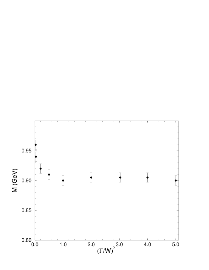
FIG. 4.: The figure shows the insensitivity of the dressed mass to the width $\Gamma$ for $\Gamma\geq W$. This case represents $g=5$ GeV, and $mT=40$. Results were obtained averaging about 4 Monte-Carlo runs at each $\Gamma$.

As a result of the scaling Eq. (62) the interaction term disappears at large $s$ values where the integrand does not contribute anyway. The benefit of this replacement is in the fact that even though N is kept finite one can perform a Wick rotation rigorously in variable $s$ to find a nonoscillatory and finite integral. Now let us take a closer look at the Wick rotation.

After the redefinition given in Eq. (62) the $s$ integral in Eq. (56) takes the following form

$$G\propto\int_{0}^{\infty}\frac{ds}{s^{2N}}\,\,{\rm exp}\biggl{[}im^{2}s-i\frac{k^{2}}{4s}-g^{2}s^{2}/R^{2}(s)\,v\biggr{]}.$$ (66)

The exponent has a singularity in the complex $s$ plane at $s_{p}=is_{0}\pm\Gamma$. One of these singularities is on the path of the Wick rotation. However it can easily be seen that it does not contribute to the integral. In particular, the contribution of the singularity at $s_{s}=is_{0}+\Gamma$, let’s call it $G_{pole}$, is given by

$$G_{pole}=i\,\frac{e^{im^{2}s_{p}-ik^{2}/(4s_{p})}}{s_{p}^{2N}}\lim_{\delta\rightarrow 0}\delta\int_{0}^{2\pi}d\theta\,{\rm exp}\biggl{[}i\theta-g^{2}s_{p}^{2}\Gamma^{2}/(4\delta^{2})e^{-2i\theta}\,v\biggr{]},$$ (67)

which is identically equal to 0. The contribution to the integral coming from the quarter circle can also be shown to vanish. On the quarter circle the interaction term approaches zero, and the integral is dominated by $1/s^{2N}$ term which vanishes as the radius of circle goes to infinity. Therefore the integral vanishes along the quarter circle. The vanishing of the interaction term on the quarter circle is only possible if one assumes that the radius of the quarter circle is much greater than $\Gamma$. Therefore $\Gamma$ can not be taken to infinity until the s integral is performed.

FIG. 5.: Wick rotation

Thus, one can indeed perform the Wick rotation without any complication to find a finite and nonoscillatory expression for the fully interacting two-body propagator:

$$G = \int_{0}^{\infty}ds\int_{0}^{\infty}d\bar{s}\int({\cal D}z)_{xy}\int({\cal D}\bar{z})_{\bar{x}\bar{y}}$$ (69)

$$\times{\rm exp}\biggl{[}-K[z,s]-K[\bar{z},\bar{s}]+V_{0}[z,s_{r}]+V_{0}[\bar{z},\bar{s}_{r}]+2V_{12}[z,\bar{z},s_{r},\bar{s}_{r}]\biggr{]},$$

where

$$s_{r}\equiv\frac{s}{R(s,s_{0})}.$$ (70)

The discretized versions of kinetic and interaction terms are given by

$$K[z,s] \rightarrow (m^{2}+i\epsilon)s-\frac{N}{4s}\sum_{i=1}^{N}(z_{i}-z_{i-1})^{2},$$ (71)

$$V_{0}[z,s] \rightarrow \frac{g^{2}s^{2}}{2N^{2}}\sum_{i,j=1}^{N}\Delta(\frac{1}{2}(z_{i}+z_{i-1}-z_{j}-z_{j-1}),\mu),$$ (72)

$$V_{12}[z,\bar{z},s,\bar{s}] \rightarrow \frac{g^{2}s\bar{s}}{2N^{2}}\sum_{i,j=1}^{N}\Delta(\frac{1}{2}(z_{i}+z_{i-1}-\bar{z}_{j}-\bar{z}_{j-1}),\mu).$$ (73)

Having outlined the treatment of the large s behavior and the Wick rotation, we next address the regularization of the ultraviolet (short distance) singularities.

B The ultraviolet regularization

The ultraviolet singularity in the kernel $\Delta(x,\mu)$ Eq. (55) can be regularized using a Pauli-Villars regularization prescription. In order to do this one replaces the kernel

$$\Delta(x,\mu)\longrightarrow\Delta(x,\mu)-\Delta(x,\alpha\mu),$$ (74)

where $\alpha$ is in principle a large constant. The ultraviolet singularity in the interaction is of the type

$$\int dz\,z\,\Delta(z,\mu).$$ (75)

At short distances the kernel $\Delta(z,\mu)$ goes as $1/z^{2}$. Therefore, we have a logarithmic type singularity. The Pauli-Villars regularization takes care of this singularity. The Pauli-Villars regularization is particularly convenient for Monte-Carlo simulations since it only involves a modification of the kernel. In order to achieve an efficient convergence in numerical simulations we use a rather small cut-off parameter $\alpha=3$. This choice leads to a less singular kernel. However this is not a major defect since the value of $\alpha$ can be increased arbitrarily at the cost additional computational time.

C Perturbation theory result for self energy

In this section we study the self energy of a particle of mass $m$ in lowest order in perturbation theory. We carry out the study in 3+1 dimension.

The lowest order “bubble” diagram is shown in Fig. 6. In 3+1 dimensions this diagram is

$$\Sigma(p)=ig^{2}\int\frac{d^{4}k}{(2\pi)^{4}}\frac{1}{\left(m^{2}-(p-k)^{2}\right)\left(\mu^{2}-k^{2}\right)}\,.$$ (76)

FIG. 6.: The self energy for $\chi^{2}\phi$ interaction.

In order to compare the perturbative result with the FSR prediction we use the same regularization method, namely the Pauli-Villars regularization. Assuming that $p^{2}<(m+\mu)^{2}$, the integration over $k$ may be rotated from the real axis to the imaginary axis without meeting any singularities. Substituting $k\to-ik$ and $p\to-ip$ and gives the Euclidean expression for the self energy

$$\Sigma_{E}(p)=-g^{2}\int\frac{d^{4}k}{(2\pi)^{4}}\frac{\Lambda^{2}-\mu^{2}}{\left(m^{2}+(p-k)^{2}\right)\left(\mu^{2}+k^{2}\right)\left(\Lambda^{2}+k^{2}\right)},$$ (77)

where the Pauli-Villars regularization mass $\Lambda$ is chosen to be $\Lambda=3\mu$. Using the Feynman trick the integral can be evaluated giving

$$\Sigma_{E}(p)=-\frac{g^{2}}{16\pi^{2}}\left[I(p^{2},\mu)-I(p^{2},\Lambda)\right],$$ (78)

where $I(p^{2},\mu)$ is defined by

$$I(p^{2},\mu) \equiv \int_{0}^{1}dx\,{\rm ln}[m^{2}x+p^{2}x(1-x)+\mu^{2}(1-x)],$$ (79)

$$= -\frac{1}{2}\biggl{[}\,2\,D\,{\rm tan}^{-1}\left(\frac{\mu^{2}-m^{2}-p^{2}}{D}\right)+(\mu^{2}-m^{2}-p^{2})\,{\rm ln}(\frac{\mu^{2}}{m^{2}})$$ (81)

$$\,\,\,\,\,\,\,\,-2\,D\,{\rm tan}^{-1}\left(\frac{\mu^{2}-m^{2}+p^{2}}{D}\right)-2p^{2}[-2+\,{\rm ln}(m^{2})]\biggr{]},$$

where

$$D\equiv\sqrt{-\mu^{4}+2\mu^{2}(m^{2}-p^{2})-(m^{2}+p^{2})^{2}}.$$ (82)

The dependence of $M$ on the coupling strength $g$ can be obtained by analytic continuation of the Euclidean form of $\Sigma$ given in Eq. (78). It is found from the on-shell condition Eq. (39) that

$$M^{2}=m^{2}-\frac{g^{2}}{16\pi^{2}}\left[I(-M^{2},\mu)-I(-M^{2},\Lambda)\right],$$ (83)

The mass $M$ is therefore the solution of this equation which must be real if the dressed mass is to be stable.

The FSR result is obtained through Monte-Carlo integration. The dressed mass $m_{0}\equiv\lim_{T\rightarrow\infty}M(T)$, which is given by Eq. (25) becomes largely independent of $T$ at large times $mT\geq 40$. As the coupling strength is increased the plateau is shifted towards higher $T$ values. In Figure 7 we demonstrate how the stability is achieved as $T$ increases for the case of $g=5$ GeV.

FIG. 7.: The Monte-Carlo result for the function $M(T)$ is shown. Error bars reflect statistical errors associated with the Monte-Carlo sampling. The plateau region occurs around $T\geq 40$.

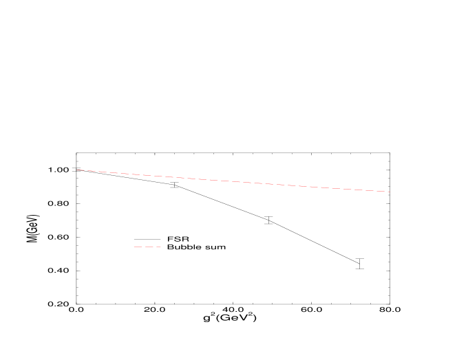
FIG. 8.: The FSR result for the function $M(g^{2})$ obtained from the Monte-Carlo simulation is shown along with the perturbative result. Error bars on the Monte-Carlo result are due to the fluctuations of the correlation function (which goes as $e^{-mt}$) under time.

The behavior of dressed mass $M(g^{2})$ as a function of the coupling constant is illustrated in Fig. 8. $M(g^{2})$ is always smaller than unity, and decreases as $g$ increases. The agreement of the FSR result with the perturbative prediction is very good at low $g^{2}\leq 30$ (GeV)². We see that the mass shift is negative, corresponding to an attractive interaction. This should be contrasted with the SQED, where a positive mass shift is predicted. From the figures we see that the higher loop contributions increase the mass shifts in both cases.

Moreover, the perturbative result displays a critical point as in the 0+1 dimension SQED case. According to the perturbative result (see Fig. 9), the dressed mass $M$ decreases up to a critical critical value $g_{\rm crit}$ which occurs when the mass reaches to $M_{\rm crit}=0.094$ GeV. For this simple case the critical coupling is given by $g_{\rm crit}=22.2$ GeV. For larger values of $g$ there are no real solutions, showing that the dressed particle is unstable. For $g>g_{\rm crit}$ the state does not propagate as a free particle. For the example shown in the figure, $m=1$ GeV, and $\mu=0.15$ GeV.

FIG. 9.: The perturbative result for the function $M(g^{2})$ is shown for $m=1$ GeV, and $\mu=0.15$. The critical coupling is given by $g_{\rm crit}=22.2$ GeV. For larger values of $g$ there are no real solutions

IV conclusions

In this paper we have considered the SQED interaction in 0+1 dimension and the scalar $\chi^{2}\phi$ interaction in 3+1 dimension. We have shown that for the SQED, the analytical FSR result and the perturbative one are in agreement at small couplings. The exact SQED result for the dressed mass is real while a lowest order bubble sum produces complex mass poles as the coupling constant is increased. This example shows that the lack of real and finite mass poles do not necessarily imply confinement unless they are obtained by fully nonperturbative calculations.

For the $\chi^{2}\phi$ interaction we have shown that it is possible to perform a Wick rotation in Feynman parameter s and obtain a convergent expression for the s integration.

V acknowledgement

This work was supported in part by the US Department of Energy under grant No. DE-FG02-97ER41032. One of us (JT) likes to thank the theory group of the Jefferson Lab for the hospitality extended to him, where this work was performed.

REFERENCES

- [1] N. Nakanishi, Prog. Theor. Phys. Suppl. 43 (1969) 1; ibid 95, 1 (1988).
- [2] P. C. Tiemeijer, J. A. Tjon, Phys. Rev. C 48 (1993); ibid C 49, 494 (1994).
- [3] F. Gross, Phys. Rev. C 26, 2203 (1982).
- [4] H. J. Rothe, ’Lattice Gauge Theory’, World Scientific 1992.
- [5] Yu. A. Simonov and J. A. Tjon, Ann. Phys. 228, 1 (1993).
- [6] T. Nieuwenhuis and J. A. Tjon, Phys. Rev. Lett. 77, 814 (1996).
- [7] N. Brambilla, A. Vairo, Phys. Rev D. 56, 1445 (1997).
- [8] P. Lepage, Proceedings of the XIV’th International Conference on Few Body Problems in Physics, Williamsburg VA, 1994 / editor Franz Gross.
- [9] T. Nieuwenhuis, PhD-thesis, University of Utrecht (1995), unpublished.
- [10] W. Pauli and G. Kallen, Dan. Mat. Fys. Medd. 30, nr. 7 (1955).
- [11] E. J. J. Kirchner and T. W. Ruijgrok, Acta Physica Polonica B22, 47 (1991).
- [12] E. van Faassen and J. A. Tjon, Phys. Rev. C 33, 2105 (1986).
- [13] Çetin Şavklı, Frank Tabakin, Nucl. Phys. A 628, 645 (1998).