IFT/99/10
hep-ph/9906206
June 1999

Constraints on Phases of Supersymmetric Flavour Conserving Couplings

S. Pokorski^a, J. Rosiek^a and C. A. Savoy^b

^aInstitute of Theoretical Physics, Warsaw University,
Hoża 69, 00-681 Warsaw, Poland
^bService de Physique Theorique, CEA Saclay,
91191 Gif-sur-Yvette CEDEX, France

Abstract

In the unconstrained MSSM, we reanalyze the constraints on the phases of supersymmetric flavour conserving couplings that follow from the electron and neutron electric dipole moments (EDM). We find that the constraints become weak if at least one exchanged superpartner mass is $>{\cal O}(1~{}\mathrm{TeV})$ or if we accept large cancellations among different contributions. However, such cancellations have no evident underlying symmetry principle. For light superpartners, models with small phases look like the easiest solution to the experimental EDM constraints. This conclusion becomes stronger the larger is the value of $\tan\beta$. We discuss also the dependence of $\epsilon_{K}$, $\Delta m_{B}$ and $b\rightarrow s\gamma$ decay on those phases.

                                           
This work was supported in part by the Polish Committee for Scientific Research under the grant numbers 2 P03B 052 16 and 2 P03B 030 14 (J.R.) and by French-Polish Programme POLONIUM.

1 Introduction

In the Minimal Supersymmetric Standard Model (MSSM) there are new potential sources of the CP non-conservation effects. One can distinguish two categories of such sources. One is independent of the physics of flavour non-conservation in the neutral current sector and the other is closely related to it. To the first category belong the phases of the parameters $\mu$, gaugino masses $M_{i}$, trilinear scalar couplings $A_{i}$ and $m_{12}^{2}$, which can in principle be arbitrary. They can be present even if the sfermion sector is flavour conserving. Not all of them are physically independent.

The other potential phases may appear in flavour off-diagonal sfermion mass matrix elements $\Delta m^{2}_{ij}$ and in flavour off-diagonal LR mixing parameters $A_{ij}$. These potential new sources of CP violation are, therefore, closely linked to the physics of flavour and, for instance, vanish in the limit of flavour diagonal (in the basis where quarks are diagonal) sfermion mass matrices. It is, therefore, quite likely that the two categories of the potential CP violation in the MSSM are controlled by different physical mechanisms. They should be clearly distinguished and discussed independently.

Experimental constraints on the “flavour-conserving” phases come mainly from the electric dipole moments of electron [1] and neutron [2]:

$$E_{e}^{exp}<4.3\cdot 10^{-27}e\cdot cm$$

$$E_{n}^{exp}<6.3\cdot 10^{-26}e\cdot cm$$

The common belief was that the constraints from the electron and neutron electric dipole moments are strong [4, 5] and the new phases must be very small. More recent calculations performed in the framework of the minimal supergravity model [6, 7, 8] indicated the possibility of cancellations between contributions proportional to the phase of $\mu$ and those proportional to the phase of $A$ and, therefore, of weaker limits on the phases in some non-negligible range of parameter space. The possibility of even more cancellations have been reported in ref. [9] in non-minimal models. For instance, for the electron dipole moment, the coefficient of the $\mu$ phase has been found to vanish for some values of parameters. Since the constraints on the supersymmetric sources of $CP$ violating phases are of considerable theoretical and phenomenological interest, in this paper we reanalyze the electric dipole moments with the emphasis on complete understanding of the mechanism of the cancellations.

The new flavour-conserving phases in the MSSM, beyond the $\theta_{QCD}$ present in the SM, may appear in the bilinear term in the superpotential and in the soft breaking terms: gaugino masses and bi- and trilinear scalar couplings - see eqs. (A.8,A.11). We define them as:

$$e^{i\phi_{\mu}}=\frac{\mu}{|\mu|}\hskip 42.67912pte^{i\phi_{i}}=\frac{M_{i}}{|M_{i}|}\hskip 42.67912pte^{i\phi_{A_{I}}}=\frac{A_{I}}{|A_{I}|}\hskip 42.67912pte^{i\phi_{H}}=\frac{m_{12}^{2}}{|m_{12}^{2}|}$$ (1)

Not all of those phases are physical. In the absence of terms (A.8,A.11) the MSSM Lagrangian has two global $U(1)$ symmetries, an $R$ symmetry and the Peccei-Quinn symmetry [10]. Terms (A.8,A.11) may be treated as spurions breaking those symmetries, with appropriate charge assignments. Physics observables depend only on the phases of parameter combinations neutral under both $U(1)$’s transformation. Such combinations are:

$$M_{i}\mu(m^{2}_{12})^{\star}\hskip 56.9055ptA_{I}\mu(m^{2}_{12})^{\star}\hskip 56.9055ptA_{I}^{\star}M_{i}$$ (2)

Not all of them are independent. The two $U(1)$ symmetries may be used to get rid of two phases. We follow the common choice and keep $m_{12}^{2}$ real in order to have real tree level Higgs field VEV’s and $\tan\beta$. The second re-phasing may be used e.g. to make one of the gaugino mass terms real - we choose it to be the gluino mass term.

A particularly simple picture is obtained assuming universal gaugino masses and universal trilinear couplings $A_{I}=A$ at the GUT scale. In this case $U(1)$’s invariant parameter combinations (2) contain at that scale only two independent phases. Defining $\phi_{g}\equiv\phi_{1}=\phi_{2}=\phi_{3}$, $\phi_{A}\equiv\phi_{A_{i}}$ we can write them down as

$$\delta_{1}=\phi_{A}-\phi_{g},\hskip 85.35826pt\delta_{2}=\phi_{g}+\phi_{\mu}-\mathrm{arg}(m_{12}^{2})$$ (3)

The re-phasing freedom may be used in this case to make all $M_{i}$ simultaneously real. The RGE for $M_{i}$ at one loop does not introduce phases once they are set to zero at GUT scale. The second $U(1)$ rotation can be used again to remove phase from $m_{12}^{2}$ already at $M_{Z}$ scale. Then only $\mu$ and $A_{I}$ parameters remain complex at electroweak scale. Phases of various $A_{I}$ parameters are not independent and can be calculated from the RGE equations.

In most of the calculations in the next sections we keep in general $\mu,M_{1},M_{2}$ and $A_{I}$ complex. As one can see, all the physical results depend explicitly only on the phases of parameter combinations (2), as follows from the general considerations above.

In Section 2 we discuss in detail the electron electric dipole moment. First, we present the results of an exact calculation, which is convenient for numerical codes. For a better qualitative understanding, we also perform the calculation in the mass insertion approximation. The results of the two methods can be compared by appropriately expanding the exact results for some special configurations of the selectron and gaugino masses. After those technical preliminaries we discuss in Section 2 the magnitude of various contributions to the electric dipole moment and investigate the pattern of possible cancellations. The first observation we want to emphasize is that, even without any cancellations, there are interesting regions in the parameter space where the phases are weakly constrained. Secondly, we do not find any symmetry principle that would guarantee cancellations in the regions where the phases are constrained. Such cancellations are, nevertheless, possible by proper tuning of the $\mu$ and $A$ phases to the values of the soft masses.

In Section 3 we analyze the neutron electric dipole moment with similar conclusions. In Section 4 we discuss the role of the $\mu$ phase in the $\epsilon_{K}$ measurement and in the $b\rightarrow s\gamma$ decay. The necessary conventions, Feynman rules and integrals are collected in the Appendices.

2 Electric dipole moment of the electron

2.1 Mass eigenstate vs. mass insertion calculation

The electric dipole moments (EDM) of leptons and quarks, defined as the coefficient $E$ of the operator

$${\cal L}_{E}=-\frac{i}{2}E\bar{\psi}\sigma_{\mu\nu}\gamma_{5}\psi F^{\mu\nu},$$ (4)

can be generated in the MSSM already at 1-loop level, assuming that supersymmetric parameters are complex.

In the mass eigenstate basis for all particles, two diagrams contribute to the electron electric dipole moment. They are shown in Fig. 1 (summation over all charginos, neutralinos, sleptons and sneutrinos in the loops is understood).

Figure 1: Diagrams contributing to lepton EDM.

The result for the lepton electric dipole moment reads:

$$E_{l}^{I} = \frac{em_{l}^{I}}{8\pi^{2}}\sum_{j=1}^{2}\sum_{K=1}^{3}m_{C_{j}}\mathrm{Im}\left((V_{l\tilde{\nu}C})_{L}^{IKj}(V_{l\tilde{\nu}C})_{R}^{IKj\star}\right)C_{11}(m_{C_{j}}^{2},m_{\tilde{\nu}_{K}}^{2})$$ (5)

$$- \frac{em_{l}^{I}}{16\pi^{2}}\sum_{j=1}^{4}\sum_{k=1}^{6}m_{N_{j}}\mathrm{Im}\left((V_{l\tilde{L}N})_{L}^{Ikj}(V_{l\tilde{L}N})_{R}^{Ikj\star}\right)C_{12}(m_{\tilde{L}_{k}}^{2},m_{N_{j}}^{2})$$

where $(V_{l\tilde{\nu}C})_{L}$, $(V_{l\tilde{\nu}C})_{R}$, $(V_{l\tilde{L}N})_{L}$, $(V_{l\tilde{L}N})_{R}$ are, respectively, the left- and right- electron-sneutrino-chargino and electron-selectron-neutralino vertices and $C_{11},C_{12}$ are the loop integrals. Explicit form of the vertices and integrals can be found in Appendix A.

The eq. (5) is completely general, but as we discussed already in the Introduction, in the rest of this paper we assume no flavour mixing in the slepton sector. Therefore, in the formulae below we skip the slepton flavour indices.

We present now the calculation of the electron EDM in the mass insertion approximation, for easier understanding of cancellations of various contributions, and then compare the two results. We use the “generalized mass insertion approximation”, i.e. we treat as mass insertions both the L-R mixing terms in the squark mass mixing matrices and the off-diagonal terms in the chargino and neutralino mass matrices. Therefore we assume that the diagonal entries in the latter: $|\mu|$, $|M_{1}|$, $|M_{2}|$ are sufficiently larger than the off-diagonal entries, which are of the order of $M_{Z}$.

There are four diagrams with wino and charged Higgsino exchange, shown in Fig. 2.

Figure 2: Chargino contribution to lepton EDM in mass insertion expansion.

Their contribution to the electron EDM is ($E_{e}\equiv E_{l}^{1}$ for electron):

$$(E_{e})_{C} = {2eg^{2}m_{e}\over(4\pi)^{2}}\mathrm{Im}(M_{2}\mu)\tan\beta{C_{11}(|\mu|^{2},m^{2}_{\tilde{\nu}})-C_{11}(|M_{2}|^{2},m^{2}_{\tilde{\nu}})\over|\mu|^{2}-|M_{2}|^{2}}$$ (6)

Neutral wino, bino and neutral Higgsino contributions can be split into two classes: with mass insertion on the fermion or on the sfermion line. Diagrams belonging to the first class are shown in Fig. 3. Their contribution has a structure very similar to that given by eq. (6):

Figure 3: Neutralino contribution to lepton EDM in mass insertion expansion: mass insertion on the fermion line.

Figure 4: Neutralino contribution to lepton EDM in mass insertion expansion: mass insertion on the scalar line

$$(E_{e})_{Nf} = -{eg^{2}m_{e}\over 2(4\pi)^{2}}\mathrm{Im}(M_{2}\mu)\tan\beta{C_{12}(m_{E}^{2},|\mu|^{2})-C_{12}(m_{E}^{2},|M_{2}|^{2})\over|\mu|^{2}-|M_{2}|^{2}}$$ (7)

$$+ {e{g^{\prime}}^{2}m_{e}\over 2(4\pi)^{2}}\mathrm{Im}(M_{1}\mu)\tan\beta{C_{12}(m_{E}^{2},|\mu|^{2})-C_{12}(m_{E}^{2},|M_{1}|^{2})\over|\mu|^{2}-|M_{1}|^{2}}$$

$$- {e{g^{\prime}}^{2}m_{e}\over(4\pi)^{2}}\mathrm{Im}(M_{1}\mu)\tan\beta{C_{12}(m_{E^{c}}^{2},|\mu|^{2})-C_{12}(m_{E^{c}}^{2},|M_{1}|^{2})\over|\mu|^{2}-|M_{1}|^{2}}$$

where we denote by $m_{E}$, $m_{{E}^{c}}$ and $m_{\tilde{\nu}}$ the masses of left- and right- selectron and electron sneutrino, respectively. Finally, diagrams with mass insertions on the selectron line are shown in Fig. 4. Only the first two with bino line in the loop give sizeable contributions. The other two with neutral Higgsino exchange are suppressed by the additional factor ${\cal O}\left(m_{e}^{2}/M_{W}^{2}\right)$ and thus completely negligible. The result is:

$$(E_{e})_{Ns} = {e{g^{\prime}}^{2}m_{e}\over(4\pi)^{2}}\mathrm{Im}\left[M_{1}(\mu\tan\beta+A_{e}^{\star})\right]{C_{12}(m_{E}^{2},|M_{1}|^{2})-C_{12}(m_{E^{c}}^{2},|M_{1}|^{2})\over m_{E}^{2}-m_{E^{c}}^{2}}$$ (8)

$$+ \mathrm{terms~{}suppressed~{}by~{}}{\cal O}\left(\frac{m_{e}^{2}}{M_{W}^{2}}\right)$$

Eqs. (6-8) have a simple structure: they are linear in the CP-invariants (2), with coefficients that are functions of the real mass parameters. Thus, the possibility of cancellations depends primarily on the relative amplitudes and signs of those coefficients. An immediate conclusion following from (6-8) is that limits on the $M_{i}\mu$ phases are inversely proportional to $\tan\beta$. Therefore, in the next Section, we discuss limits on $\sin\phi_{\mu}\tan\beta$ rather than on the $\mu$ phase itself.

The approximate formulae (6-8) work very well already for relatively small $|\mu|$, $|M_{1}|$ and $|M_{2}|$ values, not much above the $M_{Z}$ scale. Figure 5 shows the ratio of the electron EDM calculated in the mass insertion approximation to the exact 1-loop result given by eq. (5). The accuracy of the mass insertion expansion may become reasonable already for $|\mu|\geq 150$ GeV (depending on $|M_{2}/\mu|$ ratio) and becomes very good for $|\mu|\geq 200-250$ GeV.

Formulae (6-8) can also be obtained directly from the exact expression (5) using the expansion of sfermion and supersymmetric fermion mass matrices described in Appendix B (this gives a very useful cross-check of the correctness of the calculations). One should note that even though the expansion (B.75) does not work for degenerate $|M_{2}|$ and $|\mu|$, the expression (6) has already a well defined limit for $|M_{2}|=|\mu|$. The same holds for the $|M_{1}|=|\mu|$ and the degenerate sfermion masses in eqs. (7,8).

Figure 5: Ratio of the electron EDM calculated in the mass insertion approximation to the exact 1-loop result. Thinner lines: $\phi_{\mu}=0$, thicker lines: $\phi_{A}=0$. Degenerate left and right slepton masses and $M_{1}/\alpha_{1}=M_{2}/\alpha_{2}$ assumed.

2.2 Limits on $\mu$ and $A_{e}$ phases

It is useful to consider two classes of models: one with $M_{1}/\alpha_{1}=M_{2}/\alpha_{2}$ for gaugino masses, that is universal gaugino masses at the GUT scale (the universal phase can be set to zero by convention), and the other with non-universal gaugino masses and arbitrary relative phase between $M_{1}$ and $M_{2}$. In the universal case we choose $\mu$ and $A_{e}$ phases as the independent ones, in the second case the $M_{1},M_{2}$ phases are the additional free parameters. Constraints from the RGE running and proper electroweak breaking are insignificant at this point, as we have enough additional parameters to satisfy them for any chosen set of low energy values for $\mu$, $M_{1}$, $M_{2}$, $m_{E}$ and $A_{e}$

We shall begin our discussion by presenting the magnitude of each contribution (6), (7) and of the $\mu$ and $A_{e}$ terms in eq. (8), separately. For the $M_{1}/\alpha_{1}=M_{2}/\alpha_{2}$ case a sample of results is shown in Fig. 6. We identify there the parameter region where at least one of the terms is such that for $\sin\phi_{\mu}\tan\beta$ fixed at some assumed value, its contribution to $E_{e}$ is larger than $E_{e}^{exp}$. Barring potential cancellations, the fixed value of $\sin\phi_{\mu}\tan\beta$ is then the limit on this phase in the identified parameter region. In the left (right) plot of Fig. 6 we show the regions of masses (below the plotted surface) where the limits on $|\sin\phi_{\mu}|\tan\beta$ are stronger then 0.2 (0.05), respectively. We see that this region extends up to 900 (400) GeV in $m_{E}$ (physical left selectron mass) for small values of $|\mu|$ and $|M_{1}|,|M_{2}|$ (up to 200-300 GeV, say) and for larger values of $|\mu|$ and/or $|M_{1}|,|M_{2}|$ it gradually shrinks to 100 (0) GeV in $m_{E}$ for $|\mu|\sim|M_{2}|\sim 1$ TeV. We assume left and right slepton mass parameters equal, $M_{L}=M_{E}$, so that the physical masses of the left and right selectron differ by D-terms only. The regions below the plotted surfaces are the regions of interest for potential cancellations. We observe, however, that even without cancellations, there are interesting regions of small $|\mu|$ and $|M_{2}|$ and $m_{E}>{\cal O}(1\mathrm{TeV})$ or small $m_{E}$ and $|\mu|\sim|M_{2}|>{\cal O}(500~{}\mathrm{TeV})$ where the phase of $\mu$ is weakly constrained. One should also note that for very large $|\mu|$ and the other masses fixed the limits on the $\mu$ phase get stronger again. This is due to the term (8), which does not decouple for large $|\mu|$. The limits on $(|A_{e}\sin\phi_{A_{e}}|/m_{E}$ are typically significantly weaker.

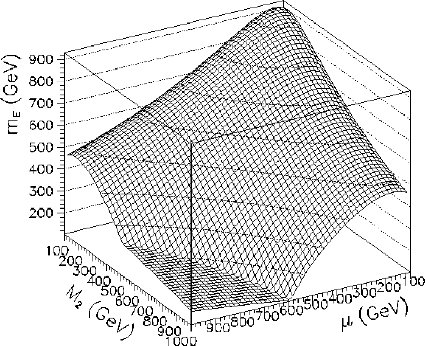
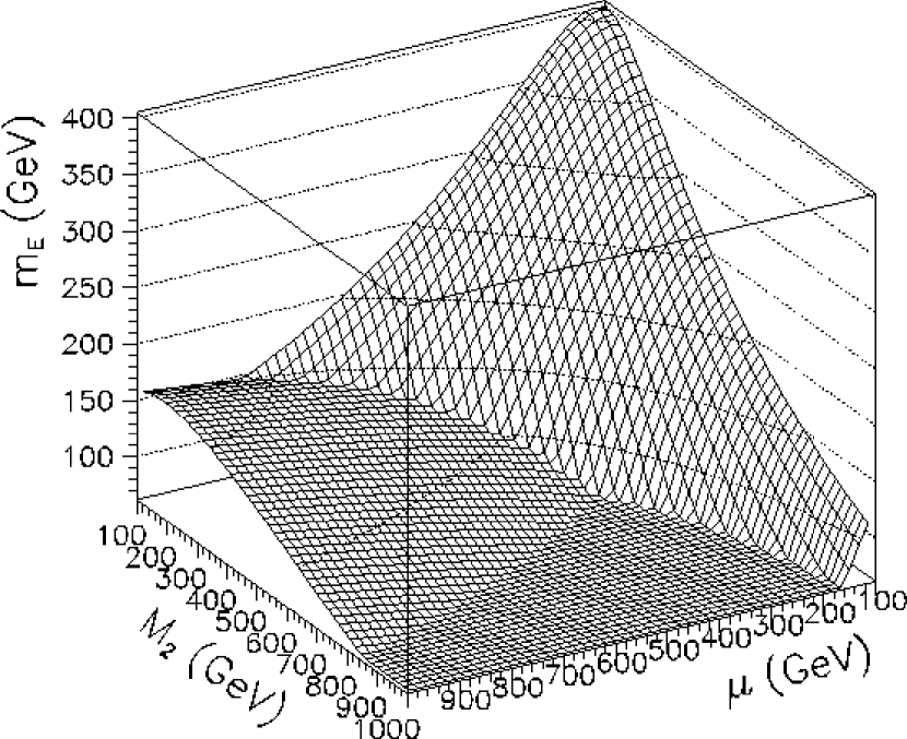
Figure 6: Regions (below the dark surface) for which generic limits on $|\sin\phi_{\mu}|\tan\beta$ are stronger then, respecively, 0.2 (left plot) and 0.05 (right plot). Degenerate left and right slepton masses and $M_{1}/\alpha_{1}=M_{2}/\alpha_{2}$ assumed.

In Fig. 7 we show again the limits on $\mu$ phase, this time as a two-dimensional plot in the $(m_{E},|M_{2}|)$ plane, assuming $M_{1}/\alpha_{1}=M_{2}/\alpha_{2}$ and $\phi_{A_{e}}=0$. The limits plotted in Fig. 7 are given by the sum of all terms (6-8), not by the largest of them like in Fig. 6.

In Fig. 8 we show similar limits on the $A_{e}$ phase on $(m_{E}$,$|M_{1}|)$ plane, assuming vanishing $\mu$ phase. The limits on the $A_{e}$ parameter phase are significantly weaker and decrease more quickly with increasing particle masses. They are almost independent of $M_{2}$ and $\mu$, as can be also seen immediately from eq. (8).

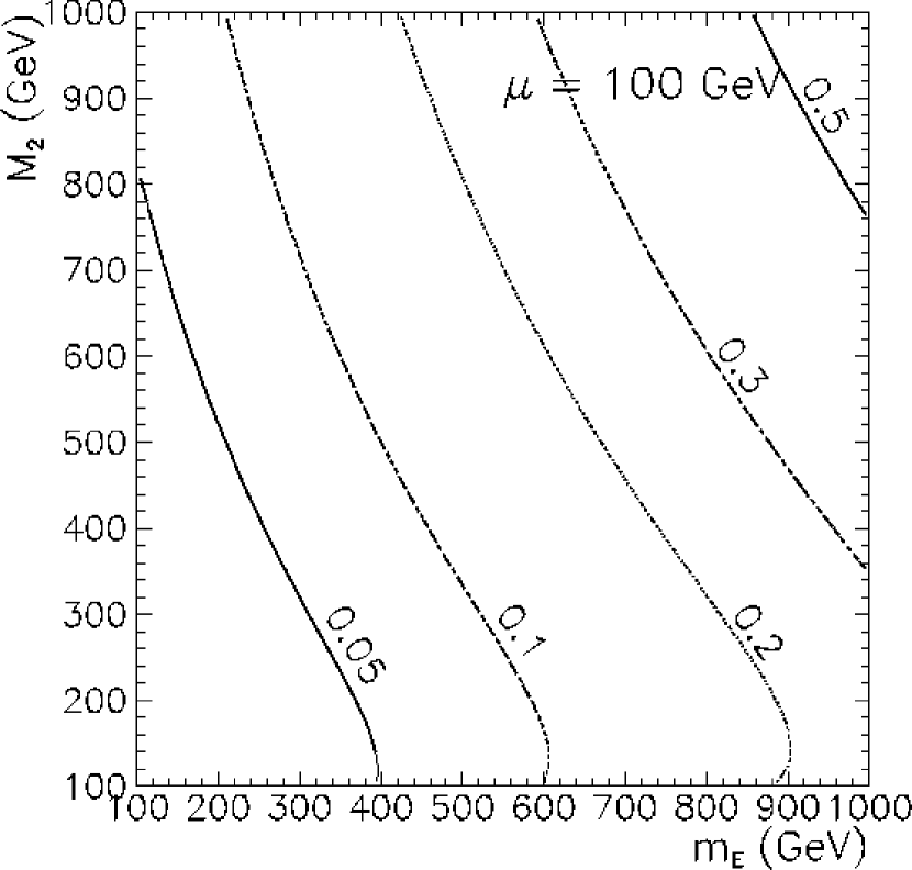
Figure 7: Limits on $|\sin\phi_{\mu}|\tan\beta$ given by the electron EDM measurements. $\sin\phi_{A_{e}}=0$ and $M_{1}/\alpha_{1}=M_{2}/\alpha_{2}$ assumed.

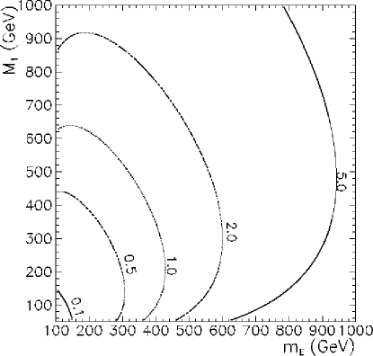
Figure 8: Limits on $|A_{e}/m_{E}\sin\phi_{A_{e}}|$ given by the electron EDM measurements ($|\mu|=200$ GeV, $\sin\phi_{\mu}=0$ and $M_{1}/\alpha_{1}=M_{2}/\alpha_{2}$ assumed).

The magnitude and signs of individual contributions as a function of $m_{E}$ are illustrated in Fig. 9. We plot there the coefficients of $\mu$ and $A_{e}$ phases obtained from the exact 1-loop result and normalized by dividing them by the experimental limit on the electron EDM. Their shape depends mostly on the $m_{E}/|\mu|$ ratio, much less on the $|\mu/M_{2}|$ ratio and scales like $1/m_{E}^{2}$. We see that either the chargino contribution to the term proportional to the $\mu$ phase dominates (for small $|\mu|$), or, if they become comparable (possible only for larger values of $|\mu|>700$ GeV), the chargino and the dominant neutralino contribution, given by eq. (8), to the $\mu$ phase coefficient are of the same sign. The neutralino contribution given by eq. (7) has opposite sign than that of eq. (8), but their sum is positive. The only exception is the case of $|\mu|,|M_{1}|\leq 100$ GeV, where both neutralino contributions are much smaller than the chargino one. Thus, the full coefficient of the $\mu$ phase cannot vanish and the only possible cancellations are between the $A_{e}$ and $\mu$ phases.

Figure 9: Relative signs and amplitudes of various contributions to the electron EDM, normalized to (divided by) the experimental limit. Solid, dashed, dotted lines: coefficients of $\sin\phi_{\mu}\tan\beta$ given by chargino (eq. (6)) and neutralino contributions (eqs. (7) and (8)) respectively. Dotted-dashed line: coefficient of $|A_{e}\sin\phi_{A_{e}}|/m_{E}$. Degenerate left and right slepton masses and $M_{1}/\alpha_{1}=M_{2}/\alpha_{2}$ assumed.

Since the $A_{e}$ phase coefficient is in the interesting region much smaller such cancellations always require large $A_{e}$ in the selectron sector, $A_{e}/m_{E}\gg 1$. This is shown in Fig. 10, where we assume “maximal” CP violation $\phi_{\mu}=\phi_{A_{e}}=\pi/2$.

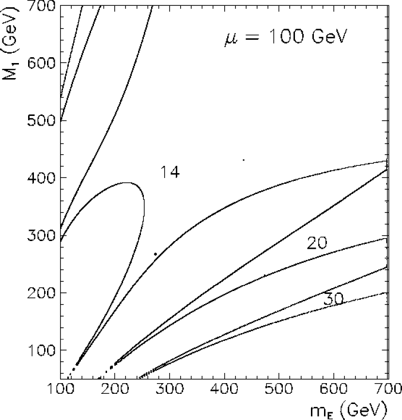
Figure 10: Regions of $m_{E}-M_{1}$ plane allowed by the electron EDM measurement assuming “maximal” CP violation $\phi_{\mu}=\phi_{A_{e}}=\pi/2$ and the corresponding values of $A_{e}/m_{E}$ parameter (marked on the plots), necessary for the $\mu-A$ cancellation.

Better understanding of the $\mu$–$A_{e}$ cancellation can be achieved after some approximations. For light supersymmetric fermions, significantly lighter than sleptons, chargino exchanges dominate (Fig. 2), whereas in the opposite limit the biggest contribution is given by the diagrams with bino exchanges (Fig. 4). Eqs. (6-8) can be greatly simplified in both cases, giving for degenerate slepton masses $m_{E}\approx m_{E^{c}}\approx m_{\tilde{\nu}}$:

1) $|M_{1,2}|,|\mu|\ll m_{E}$.

$$E_{e} \approx {eg^{2}m_{e}\over(4\pi)^{2}}{\mathrm{Im}(M_{2}\mu)\tan\beta\over m_{E}^{2}(|\mu^{2}|-|M_{2}|^{2})}\log\frac{|\mu|^{2}}{|M_{2}|^{2}}+{e{g^{\prime}}^{2}m_{e}\over 2(4\pi)^{2}}{\mathrm{Im}(M_{1}A_{e}^{\star})\over m_{E}^{4}}$$ (9)

2) $|M_{1,2}|,|\mu|\gg m_{E}$.

$$E_{e} \approx {eg^{2}m_{e}\over 4(4\pi)^{2}}{\mathrm{Im}(M_{2}\mu)\tan\beta\over|\mu|^{2}|M_{2}|^{2}}-{e{g^{\prime}}^{2}m_{e}\over 4(4\pi)^{2}}{\mathrm{Im}(M_{1}\mu)\tan\beta\over|\mu|^{2}|M_{1}|^{2}}$$ (10)

$$- {e{g^{\prime}}^{2}m_{e}\over 2(4\pi)^{2}}{\mathrm{Im}\left[M_{1}(\mu\tan\beta+A_{e}^{\star})\right]\over|M_{1}|^{4}}\left(5+2\log{m_{E}^{2}\over|M_{1}|^{2}}\right)$$

The behaviour of the lepton EDM is different in both limits. For heavy sleptons, $|M_{1,2}|,|\mu|\ll m_{E}$ the coefficient of the $\mu$ phase decreases with the increasing slepton mass as $1/m_{E}^{2}$. The coefficient of the $A_{e}$ phase decreases faster, as $1/m_{E}^{4}$. Therefore, in this limit the exact cancellation between $A_{e}$ and $\mu$ phases requires large $A_{e}$ value, growing with increasing $m_{E}$. However, because all contributions simultaneously decrease with increasing $m_{E}$, partial cancellation between $\mu$ and $A_{e}$ phase is already sufficient to push the electron EDM below the experimental limits, what may be observed in Fig. 10 as a widening of the allowed regions for large $m_{E}$.

For sufficiently small slepton masses the full cancellation between $\mu$ and $A_{e}$ terms occurs approximately for

$$\sin\phi_{A_{e}}|A_{e}|=\sin\phi_{\mu}|\mu|\tan\beta\left(1+{|M_{1}|^{2}\over|\mu|^{2}}{3\over 5+2\log\frac{m_{E}^{2}}{|M_{1}^{2}|}}\right)$$

(11)

where we assumed $M_{1}/\alpha_{1}=M_{2}/\alpha_{2}$ and redefined the $M_{1}$ phase to zero. Since this result is valid for $|\mu|,|M_{1}|,|M_{2}|\gg m_{E}$ we see that for comparable $\phi_{\mu}$ and $\phi_{A_{e}}$ the cancellation is again possible only for large $A_{e}/m_{E}\gg 1$. For large $|\mu|\gg|M_{1}|$, when one can neglect the second term in the parenthesis in eq. (11), the $A_{e}$ giving maximal cancellation is almost independent of $|M_{1}|$, what can be observed in the right plot of Fig. 10. The allowed regions also widen with increasing $|M_{1}|$, but slower then for large $m_{E}$ because the $\mu$ and $A_{e}$ phases are in this case suppressed by lower powers of $|M_{1}|$: $1/|M_{1}|$ and $1/|M_{1}|^{3}$ respectively, instead of $1/m_{E}^{2}$ and $1/m_{E}^{4}$.

It is worthwhile to note that in the most interesting region of light SUSY masses, where the limits on phases are strongest, the cancellation between (fixed) $\mu$ and $A_{e}$ phases may occur only for very precisely correlated mass parameters, i.e. it requires strong fine tuning between $|\mu|$, $|M_{1}|$, $|M_{2}|$ and $|A_{e}|$.

In Fig. 11 we plot the allowed regions of the $\phi_{A_{e}}-\phi_{\mu}$ plane for chosen fixed values of mass parameters. For light SUSY masses they are very narrow. This means that for fixed light mass parameters one needs strong fine tuning between the phases in order to fulfill experimental limits.

Figure 11: Illustration of the fine tuning between the phases for fixed mass parameters (listed in the plots), $\tan\beta=2$ and two values of $A_{e}/m_{E}=5,~{}10$ (marked near the respective allowed regions). Degenerate left and right slepton masses and $M_{1}/\alpha_{1}=M_{2}/\alpha_{2}$ assumed.

We shall discuss now the general case, with non-universal gaugino masses. The results for the magnitude of individual terms remain qualitatively similar. This is shown in Fig. 12 for $M_{1}=100$ GeV. The region of strong constraints on the $\mu$ phase shrinks in $m_{E}$ with increasing $M_{1}$. One can also see again some subtle effects like the expansion in $m_{E}$ of this region, for fixed $M_{1}$ and $M_{2}$ and increasing $|\mu|$. This behaviour can be easily understood from the analytic results of eq. (8), where one can identify the term increasing with $|\mu|$.

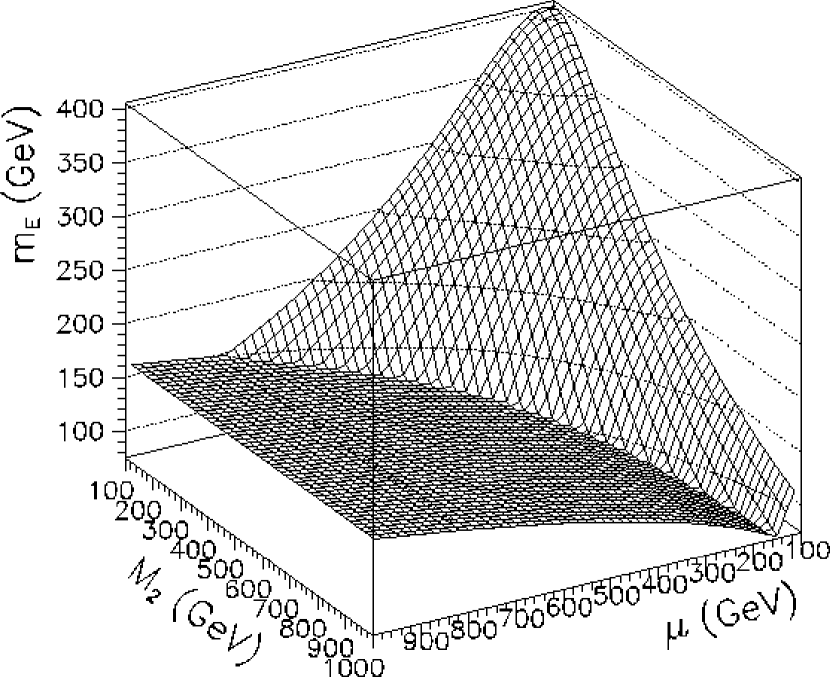
Figure 12: Regions for which generic limits on $|\sin\phi_{\mu}|\tan\beta$ are stronger then, respectively, 0.2 (left plots) and 0.05 (right plots). The plots are done for $M_{1}=100$ GeV, degenerate left and right slepton masses are assumed.

The magnitude of individual contributions as a function of $m_{E}$ has very similar behaviour as in the universal case – again, for small $|\mu|$ chargino contribution dominates for all values of $|M_{1}|$ and $|M_{2}|$. The only possible cancellations for this $|\mu|$ range are between $\mu$ and $A_{e}$ phases. For larger values of $|\mu|>700$ GeV the magnitude of individual terms may become comparable. For instance the $\mu$ phase coefficients in $E_{c}$ and $E_{Ns}$ terms (eqs. (6,8)) becomes comparable for $|\mu|/m_{E}$ fixed by the ratio $|M_{1}/M_{2}|$. With arbitrary relative phase of $M_{1}$ and $M_{2}$ it is possible to cancel the terms proportional to the $\mu$ phase. To study this possibility it is more convenient to plot the contributions proportional to $\mathrm{Im}(\mu M_{1})$ and $\mathrm{Im}(\mu M_{2})$ (Fig. 13).

Figure 13: Relative signs and amplitudes of various contributions to the electron EDM, normalized to (divided by) the experimental limit. Solid, dashed and dotted lines: coefficients of $\sin(\phi_{\mu}+\phi_{2})\tan\beta$, $\sin(\phi_{\mu}+\phi_{1})\tan\beta$ and $|A_{e}|/m_{E}\sin(\phi_{A_{e}}-\phi_{1})$ respectively. $|M_{1}|=|M_{2}|=100$ GeV and degenerate left and right slepton masses assumed.

They are comparable for $m_{E}/|\mu|\sim 1/5-1/3$, depending on $|M_{1}/M_{2}|$ ratio. It is clear that choosing $\phi_{1}$ and $\phi_{2}$ phases such that $\sin(\phi_{\mu}+\phi_{2})$ and $\sin(\phi_{\mu}+\phi_{1})$ have opposite signs, e.g. $\phi_{1}-\phi_{2}\sim\pi$, would give cancellation at these points.

To give a more specific example, lets assume $\phi_{2}=0$ and maximal $\phi_{\mu}=\pi/2$ (one can always achieve $\phi_{2}=0$ by field redefinition). In such a case, this new possibility of cancellation applies for $|\phi_{1}-\phi_{2}|\equiv|\phi_{1}|>\pi/2$. For very light $|M_{1}|$ and $m_{E}$, $|\phi_{1}|\sim\pi/2$ is required, in order to suppress the term proportional to $\mathrm{Im}(\mu M_{1})$. For heavier $M_{1}$ and $m_{E}$ to avoid limits on $\phi_{\mu}$ one needs $|\phi_{1}|\sim\pi$ – otherwise the $\mathrm{Im}(\mu M_{1})$ term is suppressed too strongly. This behaviour is illustrated in Fig. 14.

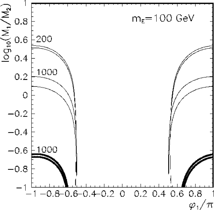
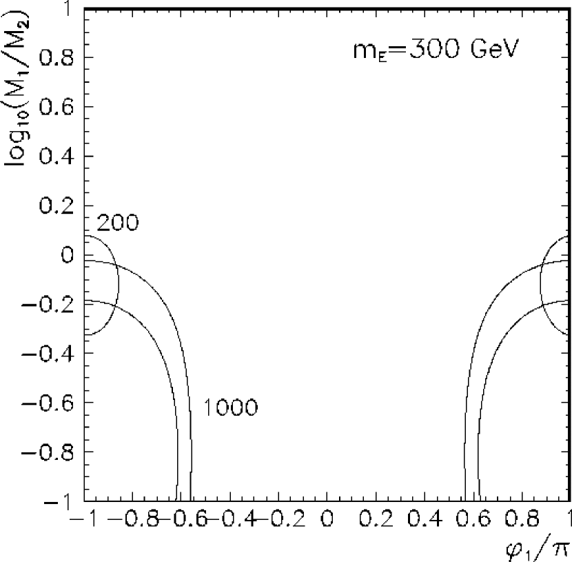
Figure 14: Allowed regions for $M_{1}$ phase as a function of $|M_{1}/M_{2}|$ for some choices of mass parameters, $\tan\beta=2$ and $\phi_{\mu}=\pi/2$. Thicker lines: $|\mu|=200$ GeV, thinner lines: $|\mu|=1000$ GeV. $|M_{2}|=200$ or $1000$ GeV (marked on the plots), $\phi_{2}=\phi_{A_{e}}=0$ and degenerate left and right slepton masses assumed.

3 EDM of the neutron

3.1 Formulae for the neutron EDM

The structure of the neutron EDM is more complicated then in the electron case. It can be approximately calculated as the sum of the electric dipole moments of the constituent $d$ and $u$ quarks plus additional contributions coming from the chromoelectric dipole moments of quarks and gluons. The chromoelectric dipole moment $C_{q}$ of a quark is defined as:

$${\cal L}_{C}=-\frac{i}{2}C_{q}\bar{q}\sigma_{\mu\nu}\gamma_{5}T^{a}qG^{\mu\nu a}$$ (12)

The gluonic dipole moment $C_{g}$ is defined as:

$${\cal L}_{g}=-\frac{1}{6}C_{g}f_{abc}G^{a}_{\mu\rho}G^{b\rho}_{\nu}G^{c}_{\lambda\sigma}\epsilon^{\mu\nu\lambda\sigma}$$ (13)

As an example, in Fig. 15 we list the diagrams contributing to the $d$-quark electric dipole moment.

Figure 15: Diagrams contributing to $d$-quark EDM.

Exact calculation of the neutron EDM requires the full knowledge of its wave function. We use the “naive” chiral quark model approximation [12], which gives the following expression:

$$E_{n}=\frac{\eta_{e}}{3}(4E_{d}-E_{u})+\frac{e\eta_{c}}{4\pi}(4C_{d}-C_{u})+\frac{e\eta_{g}\Lambda_{X}}{4\pi}C_{g}$$ (14)

where $\eta_{i}$ and $\Lambda_{X}$ are the QCD correction factors and chiral symmetry breaking scale, respectively, $\eta_{e}\approx 1.53$, $\eta_{c}\approx\eta_{g}\approx 3.4$ [13], $\Lambda_{X}=1.19$ GeV [12]. We use also following values of light quark masses: $m_{d}(\Lambda_{X})=10$ MeV, $m_{u}(\Lambda_{X})=7$ MeV [14].

Eq. (14) contains sizeable theoretical uncertainities due to non-perturbative strong interactions. However, as we show in the next section, for most parameter choices $E_{d}$ alone gives the leading contribution to the neutron EDM. Therefore, one may hope that those uncertainities affect mainly the overall normalization of the neutron EDM. They do not affect significantly the possible cancellations between the phases (or in their coefficients), as long as such cancellations must occur predominantly inside the $E_{d}$. For instance, if one uses relativistic quark-parton model [15, 8] instead of the naive chiral quark model, the contribution of quarks to the neutron EDM is weighted by [15] their contributions $\Delta_{q}$ to the spin of proton, measured in polarized lepton-nucleon scattering: $E_{n}=\eta_{e}(\Delta_{u}E_{d}+\Delta_{d}E_{u}+\Delta_{s}E_{s})$. For the neutron, applying the isospin relations, we have $(\Delta_{u})_{n}=\Delta_{d}$, $(\Delta_{d})_{n}=\Delta_{u}$, $(\Delta_{s})_{n}=\Delta_{s}$. With the assumption of degenerate masses and phases of the $A$ parameters of the first two generations of squarks, $E_{d}$ and $E_{s}$ have exactly the same structure and differ only by the quark mass multiplying the appropriate loop integrals: $E_{d}/m_{d}=E_{s}/m_{s}$ (see eq. (B.80)). Therefore, accepting the values given in ref. [16]: $\Delta_{u}=0.82$, $\Delta_{d}=-0.44$, $\Delta_{s}=-0.11$, one can estimate that, in the quark-parton model, the contribution from the $s$ sea-quark, not present at all in the naive chiral model, is predicted to dominate. The leading contributions to the neutron EDM in the considered models are (we assume $m_{s}\approx 150$ MeV):

$$\mathrm{Chiral~{}quark~{}model:} E_{n}\approx\frac{4}{3}\eta_{e}E_{d}\approx 1.33\eta_{e}E_{d}$$

$$\mathrm{Quark~{}parton~{}model:} E_{n}\approx(\Delta_{u}+\frac{m_{s}}{m_{d}}\Delta_{s})\eta_{e}E_{d}\approx-0.83\eta_{e}E_{d}$$ (15)

and the $u$ quark contribution is smaller. The coefficients of $E_{d}$ for the two models differ in magnitude and even in sign but in both models the limits on the phases can be avoided if the $E_{d}$ itself vanishes due to some internal cancellations. Of course, one should remember that the estimate (15) is subject to some uncertainity in $\Delta_{s}$ and a larger cancellation between $d$ and $s$ quark contributions, leading (at least in the low $\tan\beta$ region [15]) to the dominance of the $u$ quark contribution, is not excluded. Thus, there are uncertainities related to the choice of a particular quark model and uncertainities within the chosen model (like e.g. $\mathrm{Im}A_{d}=\mathrm{Im}A_{s}$ assumption). Any theoretical calculation of the overall normalization of the neutron EDM should be considered as a qualitative one. The pattern of cancellations we discuss in the naive chiral quark model can be more generally trusted to the extend the smallness of the $u$ quark contribution compared to the $d$ and $s$ quark contributions can be trusted as a model independent feature. At present the limits on the phases given by the electron EDM are more precise and better established.

It was recently pointed out [17] that 2-loop contributions to the neutron EDM may be numerically significant, especially for large $\tan\beta$ regime. Unlike most of the terms in eq. (14), they depend mainly on the masses and mixing parameters of the third generation of squarks. Therefore, they are especially important in the case of the third generation of squarks significantly lighter than the first two generation, so that the 1-loop contributions are suppressed. We do not include such corrections in the present analysis.

The formulae for the up- and down quark electric dipole moment are the following:

$$E_{d}^{I} = \frac{e}{8\pi^{2}}\sum_{j=1}^{2}\sum_{k=1}^{6}m_{C_{j}}\mathrm{Im}\left((V_{d\tilde{U}C})_{L}^{Ikj}(V_{d\tilde{U}C})_{R}^{Ikj\star}\right)\left(C_{11}(m_{C_{j}}^{2},m_{\tilde{U}_{k}}^{2})+\frac{1}{3}C_{12}(m_{\tilde{U}_{k}}^{2},m_{C_{j}}^{2})\right)$$ (16)

$$- \frac{e}{48\pi^{2}}\sum_{j=1}^{4}\sum_{k=1}^{6}m_{N^{0}_{j}}\mathrm{Im}\left((V_{d\tilde{D}N})_{L}^{Ikj}(V_{d\tilde{D}N})_{R}^{Ikj\star}\right)C_{12}(m_{\tilde{D}_{k}}^{2},m_{N^{0}_{j}}^{2})$$

$$- \frac{2e\alpha_{s}}{9\pi}|M_{3}|\sum_{k=1}^{6}\mathrm{Im}(Z_{DL}^{Ik}Z_{DR}^{Ik\star})C_{12}(m_{\tilde{D}_{k}}^{2},|M_{3}|^{2})$$

$$E_{u}^{I} = -\frac{e}{8\pi^{2}}\sum_{j=1}^{2}\sum_{k=1}^{6}m_{C_{j}}\mathrm{Im}\left((V_{u\tilde{D}C})_{L}^{Ikj}(V_{u\tilde{D}C})_{R}^{Ikj\star}\right)\left(C_{11}(m_{C_{j}}^{2},m_{\tilde{D}_{k}}^{2})+\frac{1}{6}C_{12}(m_{\tilde{D}_{k}}^{2},m_{C_{j}}^{2})\right)$$ (17)

$$+ \frac{e}{24\pi^{2}}\sum_{j=1}^{4}\sum_{k=1}^{6}m_{N^{0}_{j}}\mathrm{Im}\left((V_{u\tilde{U}N})_{L}^{Ikj}(V_{u\tilde{U}N})_{R}^{Ikj\star})C_{12}(m_{\tilde{U}_{k}}^{2},m_{N^{0}_{j}}^{2}\right)$$

$$+ \frac{4e\alpha_{s}}{9\pi}|M_{3}|\sum_{k=1}^{6}\mathrm{Im}(Z_{UL}^{Ik}Z_{UR}^{Ik\star})C_{12}(m_{\tilde{U}_{k}}^{2},|M_{3}|^{2})$$

Chromoelectric dipole moments of the quarks are given by:

$$C_{d}^{I} = \frac{g_{s}}{16\pi^{2}}\sum_{j=1}^{2}\sum_{k=1}^{6}m_{C_{j}}\mathrm{Im}\left((V_{d\tilde{U}C})_{L}^{Ikj}(V_{d\tilde{U}C})_{R}^{Ikj\star}\right)C_{12}(m_{\tilde{U}_{k}}^{2},m_{C_{j}}^{2})$$ (18)

$$+ \frac{g_{s}}{16\pi^{2}}\sum_{j=1}^{4}\sum_{k=1}^{6}m_{N^{0}_{j}}\mathrm{Im}\left((V_{d\tilde{D}N})_{L}^{Ikj}(V_{d\tilde{D}N})_{R}^{Ikj\star}\right)C_{12}(m_{\tilde{D}_{k}}^{2},m_{N^{0}_{j}}^{2})$$

$$- \frac{g_{s}^{3}}{8\pi^{2}}|M_{3}|\sum_{k=1}^{6}\mathrm{Im}(Z_{DL}^{Ik}Z_{DR}^{Ik\star})\left(3C_{11}(|M_{3}|^{2},m_{\tilde{D}_{k}}^{2})+\frac{1}{6}C_{12}(m_{\tilde{D}_{k}}^{2},|M_{3}|^{2})\right)$$

$$C_{u}^{I} = \frac{g_{s}}{16\pi^{2}}\sum_{j=1}^{2}\sum_{k=1}^{6}m_{C_{j}}\mathrm{Im}\left((V_{u\tilde{D}C})_{L}^{Ikj}(V_{u\tilde{D}C})_{R}^{Ikj\star}\right)C_{12}(m_{\tilde{D}_{k}}^{2},m_{C_{j}}^{2})$$ (19)

$$+ \frac{g_{s}}{16\pi^{2}}\sum_{j=1}^{4}\sum_{k=1}^{6}m_{N^{0}_{j}}\mathrm{Im}\left((V_{u\tilde{U}N})_{L}^{Ikj}(V_{u\tilde{U}N})_{R}^{Ikj\star}\right)C_{12}(m_{\tilde{U}_{k}}^{2},m_{N^{0}_{j}}^{2})$$

$$- \frac{g_{s}^{3}}{8\pi^{2}}|M_{3}|\sum_{k=1}^{6}\mathrm{Im}(Z_{UL}^{Ik}Z_{UR}^{Ik\star})\left(3C_{11}(|M_{3}|^{2},m_{\tilde{U}_{k}}^{2})+\frac{1}{6}C_{12}(m_{\tilde{U}_{k}}^{2},|M_{3}|^{2})\right)$$

Finally, the gluon chromoelectric dipole moment is given by:

$$C_{g} = {3\alpha_{s}^{2}g_{s}m_{t}\over 16\pi^{2}}\mathrm{Im}(Z_{UL}^{36\star}Z_{UR}^{36}){m_{\tilde{t}_{1}}^{2}-m_{\tilde{t}_{2}}^{2}\over|M_{3}|^{5}}H\left({m_{\tilde{t}_{1}}^{2}\over|M_{3}|^{2}},{m_{\tilde{t}_{2}}^{2}\over|M_{3}|^{2}},{m_{t}^{2}\over|M_{3}|^{2}}\right)$$ (20)

where the definition of the 2-loop function $H$ can be found in [18].

The full form of all necessary fermion-sfermion-chargino/neutralino vertices can be found in Appendix A. In Appendix B we give also mass insertion expressions for the quark electric and chromoelectric dipole moments. Although somewhat more complicated than in the case of leptons, they are very useful for qualitative understanding of the neutron EDM behaviour.

3.2 Limits on phases

The neutron EDM depends on more phases than the electron EDM. All electric and chromoelectric dipole moments depend on the common $\mu$ phase, but some of them are proportional to $\mu\tan\beta$ and others to $\mu\cot\beta$, hence the limit on $\mu$ phase does not scale simply like $1/\tan\beta$, as it was in the electron case. In addition, the quark moments depend on the phases of the two LR mixing parameters of the first generation of squarks, $A_{d}$ and $A_{u}$. The gluonic chromoelectric dipole moment depends in principle on all $A$ parameters and squark masses, but contributions from different squark generation are weighted by the respective fermion mass, so we take into account only the dominant stop contribution, dependent on the $A_{t}$ parameter.

In practice, the analysis of the dependence of the neutron EDM on SUSY parameters appears less complicated than suggested by the above list, as some of the parameters have small numerical importance. As discussed below, the result is most sensitive to the squark masses of the first generation (left and right), gaugino masses, $|\mu|$, $A_{u}$, $A_{d}$ and $\tan\beta$.

The number of free parameters can be further reduced by assuming GUT unification with universal boundary conditions. Such a variant was thoroughly discussed in [7, 8], so we do not repeat the full RGE analysis here, however its results can be qualitatively read also from the figures presented in this section. This can be done with the use of the following observations:

• As mentioned above, the neutron EDM is sensitive mostly to the masses of the first generation of squarks. Assuming universal sfermion masses at the GUT scale one can to a good approximation keep them degenerate also at $M_{Z}$ scale. The remnant of the GUT evolution is their relation to the gaugino masses: $m_{Q}^{2}\approx m_{D}^{2}\approx m_{U}^{2}\approx m_{0}^{2}+6.5M_{1/2}^{2}\approx m_{0}^{2}+10|M_{2}|^{2}$, which leads to the relation $m_{Q}\approx m_{U}\approx m_{D}\geq 3M_{2}$.

• The $\mu$ phase does not run. The $\mu$ itself runs weakly, it means that $\mathrm{Im}\mu$ also runs weakly. It is a free parameter anyway.

• The imaginary parts of the first generation $A$ parameters, $\mathrm{Im}A_{u}$ and $\mathrm{Im}A_{d}$, do not run, apart from the small corrections proportional to the Yukawa couplings of light fermions. Real parts of $A_{u}$ and $A_{d}$ run approximately in the same way. Therefore universal boundary conditions at the GUT scale lead simply to $\phi_{A_{u}}=\phi_{A_{d}}$ at the $M_{Z}$ scale.

• RGE running suppresses the $A_{t}$ phase (present in the chromoelectric dipole moment of gluons $C_{g}$). Therefore, the low energy constraints are easy to satisfy even with large $\phi_{A_{t}}$ at the GUT scale. The limits on $\phi_{A_{t}}$ at the electroweak scale appear themeselves to be rather weak.

• With universal gaugino masses and phases, $M_{1}/\alpha_{1}=M_{2}/\alpha_{2}=M_{3}/\alpha_{3}$, the common gaugino phase can be completely rotated away.

Using i)-v) one can use our plots for the universal GUT case, just assuming common $A$ phase, neglecting $\phi_{A_{t}}$ and looking at the part of plots for which $m_{Q}\geq 3M_{2}$. Actually, in all Figures of this Section we keep degenerate squark mass parameters $M_{Q}=M_{D}=M_{U}$, so that the physical masses differ by D-terms only. We plot the results in terms of the physical mass of the $D$-squark $m_{D}$.

We consider first the limits on the $\mu$ phase, neglecting the possibility of $\mu-A$ cancellations. In Fig. 16 (analogous to Fig. 6) we show where the generic limits for the $\mu$ phase given by the neutron EDM are strong. We plot there the area where the limit on $|\sin\phi_{\mu}|\tan\beta$ given separately by each of the contributions present in eq.(14) is stronger then 0.2 or 0.05 (in addition we consider separately the chargino, neutralino and gluino contributions to $E_{d}$). For small $|\mu|$, $|M_{2}|$, squark masses $m_{Q}\sim m_{D}\sim m_{U}>1600(750)$ GeV are required to avoid the assumed limits.

Figure 16: Regions for which generic limits on $|\sin\phi_{\mu}|\tan\beta$ given by neutron EDM are stronger then, respecively, 0.2 (left plot) and 0.05 (right plot). Degenerate squark masses and GUT related $M_{1},M_{2},M_{3}$ assumed.

The dominant contributions to the coefficient multiplying $\sin\phi_{\mu}$ come from the first term of eq. (14), i.e. from the d-quark electric dipole moment, as illustrated in Fig. 17. The only exception is large $|\mu|$ and light gauginos case, where also $C_{d}$ becomes comparable to the other term. In principle, relative importance of various contributions changes with $\tan\beta$, as $E_{d},C_{d}$ are proportional to $\mu\tan\beta$ and $E_{u},C_{u},C_{g}$ to $\mu\cot\beta$. However, $E_{d}$ and eventually $C_{d}$ always dominate and the $\mu$ phase coefficient scales again, like in the electron case, as $\tan\beta$ (Fig. 17 has been done for $\tan\beta=2$).

Figure 17: Contributions to $\sin\phi_{\mu}\tan\beta$ coefficient in the neutron EDM, normalized to (divided by) the experimental limit. Solid, dashed, dotted line: chargino, neutralino and gluino contributions to $E_{d}$; dotted-dashed line: $E_{u}+C_{d}+C_{u}+C_{g}$ summed up. $|M_{2}|=100$ GeV, $M_{1},M_{2},M_{3}$ GUT-related, $\phi_{A_{i}}=0$ and degenerate squark masses assumed.

The largest contributions to $\mu$ phase coefficient are given by the chargino and gluino (for small and large $|\mu|$, respectively) diagrams. They have the same sign, so again, like in the electron case, the total $\mu$ phase coefficient may disappear only if one allows the non-universal gaugino phases. The limits on $|\sin\phi_{\mu}|\tan\beta$ on $m_{D}-|M_{2}|$ plane are plotted in Fig. 18.

Figure 18: Limits on $|\sin\phi_{\mu}|\tan\beta$ given by the neutron EDM measurements. $M_{1},M_{2},M_{3}$ GUT-related, $\phi_{A_{u}}=\phi_{A_{d}}=\phi_{A_{t}}=0$ and degenerate squark masses assumed.

Some differences with the electron case may be observed in the structure of possible $\mu-A$ cancellations. For $E_{e}$ the term proportional to $A_{e}$ originates from the neutralino exchange diagram. For the neutron, additional contributions proportional to $A_{u}$, $A_{d}$ and $A_{t}$ are given by the diagrams with gluino exchange and they have larger magnitude than those induced by neutralino loops, as illustrated in Fig. 19 (this efect is particularly strong for large $|\mu|$ and light gauginos).

Figure 19: Coefficients of $\sin\phi_{\mu}\tan\beta$, $|A_{d}|/m_{D}\sin\phi_{A_{d}}$, $|A_{u}|/m_{U}\sin\phi_{A_{u}}$ and $|A_{t}|/m_{T}\sin\phi_{A_{t}}$ terms in the neutron EDM (solid, dashed, dotted and dashed-dotted lines respectively). $M_{1},M_{2},M_{3}$ GUT-related and degenerate squark masses assumed.

This means that, on the one hand constraints on the $A_{I}$ phases are somewhat stronger than in the electron case but, on the other hand, smaller $A_{I}$ values are necessary for cancellations. For small $|\mu|\sim 100$ GeV one needs $A_{e}/m_{E}\geq 14$ but only $A_{d}/m_{D}\sim A_{u}/m_{U}\geq 3$. Furthermore, in unconstrained MSSM we have bigger freedom because of several different $A_{i}$ parameters present in the formulae for $E_{n}$. Contributions proportional to $A_{u},A_{t}$, coming from $E_{u},C_{u}$ and $C_{g}$, are more important comparing to those given by the $E_{d},C_{d}$ as they are not suppressed by the relative factor $\cot^{2}\beta$ (like it is for the $\mu$ phase). Therefore, one has to take into account all $A_{i}$ phases. In Fig. 20 (compare Fig. 10) we plot the regions of $m_{D}-|M_{1}|$ plane allowed by the neutron EDM measurement assuming $\phi_{\mu}=\phi_{A_{d}}=\phi_{A_{u}}=\pi/2$ and various values of $A_{u}/m_{U}=A_{d}/m_{D}$.

Figure 20: Regions of $m_{D}-|M_{1}|$ plane allowed by the neutron EDM measurement assuming “maximal” CP violation $\phi_{\mu}=\phi_{A_{d}}=\phi_{A_{u}}=\pi/2$, various values of $A_{d}/m_{D}=A_{u}/m_{U}$ (marked on the plots), $A_{t}=0$, $m_{Q}=m_{U}=m_{D}$ and $M_{1}/\alpha_{1}=M_{2}/\alpha_{2}=M_{3}/\alpha_{3}$.

The overall conlusion is that eventual cancellations in neutron EDM are more likely than in the electron case. They require somewhat smaller values of $A$ parameters when one considers $\mu-A$ phases cancellations. Furthermore, assuming non-universal $A_{i}$ parameters it is possible to suppress simultaneously both $E_{e}$ and $E_{n}$ values below the experimental constraints, at the cost of rather strong fine-tuning if the SUSY mass parameters are light.

4 $\mu$ phase dependence of $\epsilon_{K}$ , $\Delta m_{B}$ and $b\rightarrow s\gamma$ 

Analysing the dependence of $\bar{K}^{0}K^{0}$ and $\bar{B}B$ mixing on the SUSY phases, we assume that there is no flavour violation in the squark mass matrices, so that only chargino and charged Higgs contributions to the matrix element do not vanish (gluino and neutralino contributions are always proportional to the flavour off-diagonal entries in the squark mass matrices). Furthermore, only chargino exchange contribution depends on the $\mu$, $M_{2}$ and $A$ phases and is interesting for our analysis. The leading chargino contribution is proportional to the $\bar{d}_{L}^{I\alpha}\gamma_{\mu}d_{L}^{J\alpha}\cdot\bar{d}_{L}^{I\beta}\gamma_{\mu}d_{L}^{J\beta}$ matrix element and has the form:

$$(M_{C})_{LLLL}=\frac{1}{8}\sum_{i,j,k,l}(V_{d\tilde{U}C})_{L}^{Iki}(V_{d\tilde{U}C})_{L}^{Ilj}(V_{d\tilde{U}C})_{L}^{Jli\star}(V_{d\tilde{U}C})_{L}^{Jkj\star}D_{2}(m^{2}_{C_{i}},m^{2}_{C_{j}},m^{2}_{\tilde{U}_{k}},m^{2}_{\tilde{U}_{l}})$$ (21)

where one should put $I=2,J=1$ for $\bar{K}^{0}K^{0}$ mixing, $I=3,J=1$ for $\bar{B}_{d}B_{d}$ mixing and $I=3,J=2$ for $\bar{B}_{s}B_{s}$ mixing (see Appendix A for the expression for loop function $D_{2}$).

In order to analyze the dependence of the matrix element (21) on the phases, we consider the simplest case of flavour-diagonal and degenerate up-squark mass and L-R mixing matrices and $|\mu|,|M_{2}|\geq 2M_{Z}$. In this case we can expand the matrix element in the mass insertion approximation, both in the sfermion and chargino sectors, as described in Appendix B. The eq. (21) gives in such approximation:

$$(M_{C})_{LLLL} \approx \frac{1}{8}\left(K^{\dagger}Y_{u}^{2}K\right)^{2}_{JI}\left[D_{2}(|\mu|^{2},|\mu|^{2},m^{2}_{U},m^{2}_{U})\right.$$ (22)

$$+ 8M_{W}^{2}\mathrm{Re}\left[(\mu^{\star}\cos\beta+M_{2}\sin\beta)(\mu\cos\beta+A_{U}^{\star}\sin\beta)\right]$$

$$\times \left.{\partial\over\partial m^{2}_{U}}{D_{2}(|\mu|^{2},|\mu|^{2},m^{2}_{U},m^{2}_{U})-D_{2}(|\mu|^{2},|M_{2}|^{2},m^{2}_{U},m^{2}_{U})\over|\mu|^{2}-|M_{2}|^{2}}\right]$$

$\epsilon_{K}$ and $\Delta m_{B}$ are proportional, respectively, to the imaginary and real part of the matrix element. One can see immediately from the equation above that in the leading order it is sensitive only to $|\mu|$ and to the real parts of the $M_{2}\mu$, $A_{U}\mu$ and $M_{2}A_{U}^{\star}$ products, i.e. to cosins of the appropriate phase combinations, not sins of them like it was in the EDM case. Eventual effects of the phases can be thus visible only for large phase values. Even then, they are suppressed by $M_{W}^{2}/m_{\tilde{U}}^{2}$ ratio and small numerical coefficient mutiplying them. An example of the $\epsilon_{K}$ dependence on the $\mu$ and $A_{U}$ phases (based on exact expression (21) and assuming $M_{2}$ to be real) is presented in Fig. 21. As can be seen from the Figure, even for light SUSY particle masses the change of the $\epsilon_{K}$ value with variation of $\mu$ and $A$ phases is smaller than 5%.

Figure 21: Dependence of $\epsilon_{K}$ on $\mu$ and $A_{u}$ phases, normalized to $\phi_{\mu}=\phi_{A_{u}}=0$ case. Thin lines: dependence on $\phi_{\mu}$ for $\phi_{A_{u}}=0$, thick lines: dependence on $\phi_{A_{u}}$ for $\phi_{\mu}=0$.

Figure 22: Dependence of $\mathrm{Br}(B\rightarrow X_{s}\gamma)$ on $\mu$ and $A_{t}$ phases for $m_{A}=500$ GeV, $|\mu|=|M_{2}|=\alpha_{2}/\alpha_{1}|M_{1}|=200$ GeV, $m_{\tilde{t}_{L}}=300$ GeV, $m_{\tilde{t}_{R}}=100$ GeV.

Recently the potential importance of non-leading chargino contributions to $\epsilon_{K}$ and $\bar{B}B$ mixing (proportional to LLRR and RRRR matrix elements) was discussed in the literature [19]. Such contributions are suppressed by the factor $m_{s}^{2}(m_{b}^{2})\tan^{2}\beta/M_{W}^{2}$ for $\bar{K}^{0}K^{0}$ ($\bar{B}B$ ) mixing. Therefore they can be significant only for large $\tan\beta$ values. Demir et al. [19] estimate that $\mbox{$\epsilon_{K}$~{}}\sim 3\cdot 10^{-3}$ can be obtained solely due to the supersymmetric phases of $\mu$ and $A_{t}$, assuming vanishing Kobayashi-Maskawa phase $\delta_{KM}=0$. It requires however large $\tan\beta=60$, large phases $\phi_{\mu}\sim\phi_{A_{t}}\sim-\pi/2$ and light stop and chargino: in the example they give $|\mu|=|M_{2}|=125$ GeV, $m_{\tilde{t}_{L}}=m_{\tilde{t}_{R}}=150$ GeV, $|A_{t}|=250$ GeV, what gives physical masses $m_{\tilde{t}_{1}}\approx 83$ GeV, $m_{C_{1}}\approx 80$ GeV. As follows from our discussion in sections  2 and 3, it is rather unlikely, although not completely impossible, to avoid limits on $\mu$ phase for light SUSY spectrum and simultaneously large $\tan\beta$ (limits on $\mu$ phase are inversely proportional to $\tan\beta$). The generic limits are in such a case very tight, so in order to avoid them one needs strong fine tuning and large cancellations between various contributions. For example, assuming the above set of parameters, universal gaugino masses and phases, $m_{E}=m_{U}=m_{D}=200$ GeV, $A_{u}=A_{d}$, $\phi_{A_{i}}=\pi/2$ one needs very large $|A_{e}|/m_{E}\sim 750$ and $|A_{u}|/m_{U}=|A_{d}|/m_{D}\sim 170$ in order to avoid the limits from the electron and neutron EDM measurements. Alternatively, one can keep smaller $A_{i}$ but give up the assumption of gaugino mass universality and adjust precisely their masses and relative phases. In each case, a very peculiar choice of parameters is required to fulfill simultaneously experimental measurements of $\epsilon_{K}$ and EDM’s if one choose to keep $\delta_{KM}=0$.

Because of the weak dependence of $\epsilon_{K}$ and $\Delta m_{B}$ on flavour conserving supersymmetric CP phases (excluding possibly very large $\tan\beta$ case), the determination of the KM matrix phase $\delta_{KM}$ (see e.g. [21]) is basically unaffected by their eventual presence. However, one should remeber that the KM phase detemination in the MSSM depends on the chargino and charged Higgs masses and mixing angles, even if not on their phases.

In contrast to $\epsilon_{K}$ and $\Delta m_{B}$, $b\rightarrow s\gamma$ decay appears to depend strongly on the $\mu$ and $A_{t}$ phases. This is illustrated in Fig. 22. Exact formulae for the matrix element for $b\rightarrow s\gamma$ decay can be found e.g. in [21]. Expansion in the sfermion and chargino/neutralino mass insertions (assuming degenerate stop masses) gives the following approximate result for the so-called $C_{7}^{(0)}$ coefficient, which primarily defines the size of $Br(B\rightarrow X_{s}\gamma)$:

$$C_{7}^{(0)}(M_{W}) \approx -{1\over 12|\mu|^{2}\sin^{2}\beta}f_{1}({m_{\tilde{t}}^{2}\over|\mu|^{2}})-{M_{W}^{2}\over 6|M_{2}|^{4}}f_{1}^{\prime}({m_{\tilde{t}}^{2}\over|M_{2}|^{2}})-{(|\mu|^{2}\cot\beta+A_{t}\mu)\over 3|\mu|^{4}\sin 2\beta}f^{\prime}_{2}({m_{\tilde{t}}^{2}\over|\mu|^{2}})$$

$$- {M_{W}^{2}\mathrm{Re}\left[(\mu\cot\beta+A_{t}^{\star})(\mu^{\star}\cot\beta+M_{2})\right]\over 3(|M_{2}|^{2}-|\mu|^{2})}\left({f^{\prime}_{1}(\frac{m_{\tilde{t}}^{2}}{|M_{2}|^{2}})\over|M_{2}|^{4}}-{f^{\prime}_{1}(\frac{m_{\tilde{t}}^{2}}{|\mu|^{2}})\over|\mu|^{4}}\right)$$

$$- {M_{W}^{2}\over 3(|M_{2}|^{2}-|\mu|^{2})}\left[\left({f^{\prime}_{2}({m_{\tilde{t}}^{2}\over|M_{2}|^{2}})\over|M_{2}|^{2}}-{f^{\prime}_{2}({m_{\tilde{t}}^{2}\over|\mu|^{2}})\over|\mu|^{2}}\right)\tan\beta+\mu M_{2}\left({f^{\prime}_{2}({m_{\tilde{t}}^{2}\over|M_{2}|^{2}})\over|M_{2}|^{4}}-{f^{\prime}_{2}({m_{\tilde{t}}^{2}\over|\mu|^{2}})\over|\mu|^{4}}\right)\right]$$

where

$$f_{1}(x) = {x(3x-2)\over(1-x)^{4}}\log x+{8x^{2}+5x-7\over(1-x)^{3}}$$

$$f_{2}(x) = {-x(3x-2)\over(1-x)^{3}}\log x-{x(5x-3)\over 2(1-x)^{2}}$$ (24)

Expression (4) contains terms proportional to both real and imaginary parts of the $\mu$ and $A_{t}$ parameters. However, the branching ratio $Br(B\rightarrow X_{s}\gamma)$ depends on $|C_{7}^{(0)}(M_{W})|^{2}$ which, like in the $\epsilon_{K}$ case, depends mainly on the real parts of the $\mu$ and $A_{t}$ parameters, i.e. on cosins of the phases. This is clearly visible in Fig. 22. However, contrary to the $\epsilon_{K}$ case, this dependence is quite strong and growing with increase of $\tan\beta$ and of the stop LR-mixing $A_{t}$ parameter. Also, as follows from the discussion in the previous Section, the limits on $A_{t}$ phase are rather weak, independently on $\tan\beta$, so one can expect large effects of this phase in $Br(B\rightarrow X_{s}\gamma)$ decay.

5 Conclusions

In this paper we have reanalyzed the constraints on the phases of flavour conserving supersymmetric couplings that follow from the electron and neutron EDM measurements. Also, we have discussed the dependence on those phases of $\epsilon_{K}$ , $\Delta m_{B}$ and the branching ratio for $b\rightarrow s\gamma$ . We find that the constraints on the phases (particularly on the phase of $\mu$ and of the gaugino masses) are generically strong $\phi\leq 10^{-2}$ if all relevant supersymmetric masses are light, say $\leq{\cal O}(500~{}\mathrm{GeV})$. However, we also find that the constraints disappear or are substantially relaxed if just one of those masses, e.g. slepton mass, is large, $m_{E}>{\cal O}(1~{}\mathrm{TeV})$. Thus, the phases can be large even if some masses, e.g. the chargino masses, are small.

In the parameter range where the constraints are generically strong, there exist fine-tuned regions where cancellations between different contributions to the EDM can occur even for large phases. However, such cancellations have no obvious underlying symmetry principle. From the low energy point of view they look purely accidental and require not only $\mu-A$, $\mu-M_{gaugino}$ or $M_{1}-M_{2}$ phase adjustment but also strongly correlated with the phases and among themselves values of soft mass parameters. Therefore, with all soft masses, say, $\leq{\cal O}(1~{}\mathrm{TeV})$ models with small phases look like the easiest solution to the experimental EDM constraints. This conclusion becomes stronger the higher is the value of $\tan\beta$, as the constraints on $\mu$ phase scale as $1/\tan\beta$, and will be substantially stronger also for low $\tan\beta$ after order of magnitude improvements in the experimental limits on EDM’s. Nevertheless, since the notion of fine tuning is not precise, particularly from the point of view of GUT models, it is not totally inconceivable that the rationale for large cancellations exists in the large energy scale physics (in a very recent paper [22] it is pointed out that non-universal gaugino phases necessary (but not sufficient) for large cancellations can be obtained in some String I type models). Therefore all experimental bounds on the supersymmetric parameters, and particularly on the Higgs boson masses [23], should include the possibility of large phases even if with large cancellations, to claim full model independence.

The dependence of $\epsilon_{K}$ and $\Delta m_{B}$ on the supersymmetric phases is weak and gives no clue about their values. Hence, the $\delta_{KM}$ determination remains essentially unaffected. Large effects may be observed in $b\rightarrow s\gamma$ decay, but, apart from the $\phi_{\mu}$ and $\phi_{A_{t}}$ phases, $b\rightarrow s\gamma$ amplitude depends on many free mass parameters, including the Higgs mass and the masses of squarks of the third generation.

Appendix A Conventions and Feynman rules

For easy comparison with other references we spell out our conventions. They are similar to the ones used in ref. [24]. The MSSM matter fields form chiral left-handed superfields in the following representations of the $SU(3)\times SU(2)\times U(1)$ gauge group (the generation index is suppressed):

$$\begin{array}[]{lll}\mathrm{Scalar~{}field}&\mathrm{Weyl~{}Fermion~{}field}&SU(3)\times SU(2)\times U(1)~{}\mathrm{representation}\\ L=\left(\begin{array}[]{c}\tilde{\nu}_{0}\\ E\end{array}\right)&\mbox{\hskip 28.45274pt}l=\left(\begin{array}[]{c}{\nu}\\ e\end{array}\right)&\mbox{\hskip 56.9055pt}(0,2,-1)\\ E^{c}&\mbox{\hskip 28.45274pt}e^{c}&\mbox{\hskip 56.9055pt}(0,0,2)\\ Q=\left(\begin{array}[]{c}U\\ D\end{array}\right)&\mbox{\hskip 28.45274pt}q=\left(\begin{array}[]{c}u\\ d\end{array}\right)&\mbox{\hskip 56.9055pt}(3,2,\frac{1}{3})\\ D^{c}&\mbox{\hskip 28.45274pt}d^{c}&\mbox{\hskip 56.9055pt}(\bar{3},0,\frac{2}{3})\\ U^{c}&\mbox{\hskip 28.45274pt}u^{c}&\mbox{\hskip 56.9055pt}(\bar{3},0,-\frac{4}{3})\\ H^{1}\left(\begin{array}[]{c}H_{1}^{1}\\ H_{2}^{1}\end{array}\right)&\mbox{\hskip 28.45274pt}\tilde{h}^{1}\left(\begin{array}[]{c}\tilde{h}_{1}^{1}\\ \tilde{h}_{2}^{1}\end{array}\right)&\mbox{\hskip 56.9055pt}(0,2,-1)\\ H^{2}\left(\begin{array}[]{c}H_{1}^{2}\\ H_{2}^{2}\end{array}\right)&\mbox{\hskip 28.45274pt}\tilde{h}^{2}\left(\begin{array}[]{c}\tilde{h}_{1}^{2}\\ \tilde{h}_{2}^{2}\end{array}\right)&\mbox{\hskip 56.9055pt}(0,2,1)\end{array}$$

Two $SU(2)$-doublets can be contracted into an $SU(2)$-singlet, e.g. $H^{1}H^{2}=\epsilon_{ij}H^{1}_{i}H^{2}_{j}=-H^{1}_{1}H^{2}_{2}+H^{1}_{2}H^{2}_{1}$ (we choose $\epsilon_{12}=-1$; lower indices (when present) will label components of $SU(2)$-doublets). The superpotential and the soft terms are defined as:

$$W=W_{0}+W_{CP}$$ (A.6)

$$W_{0}=Y_{e}H^{1}LE+Y_{d}H^{1}QD+Y_{u}H^{2}QU$$ (A.7)

$$W_{CP}=\mu H^{1}H^{2}$$ (A.8)

$${\cal L}_{soft} = {\cal L}_{soft-0}+{\cal L}_{soft-CP}$$ (A.9)

$${\cal L}_{soft-0} = -M_{H^{1}}^{2}H^{1\dagger}H^{1}-M_{H^{2}}^{2}H^{2\dagger}H^{2}-L^{\dagger}M_{L}^{2}L-E^{c\dagger}M_{E}^{2}E^{c}$$ (A.10)

$$-Q^{\dagger}M_{Q}^{2}Q-D^{c\dagger}M_{D}^{2}D^{c}-U^{c\dagger}M_{U}^{2}U^{c}$$

$${\cal L}_{soft-CP} = \frac{1}{2}\left(M_{3}\tilde{G}^{a}\tilde{G}^{a}+M_{2}\tilde{W}^{i}\tilde{W}^{i}+M_{1}\tilde{B}\tilde{B}\right)+m^{2}_{12}H^{1}H^{2}$$ (A.11)

$$+Y_{e}A_{e}H^{1}LE^{c}+Y_{d}A_{d}H^{1}QD^{c}+Y_{u}A_{u}H^{2}QU^{c}+\mathrm{H.c.}$$

where we divided all terms into two subclasses, collecting in $W_{CP}$ and ${\cal L}_{soft-CP}$ those of them which may contain flavour-diagonal CP breaking phases. We also extracted Yukawa coupling matrices from the definition of the $A_{I}$ coefficients.

In general, the Yukawa couplings and the masses are matrices in the flavour space. Rotating the fermion fields one can diagonalize the Yukawa couplings (and simultaneously fermion mass matrices). This procedure is well known from the Standard Model: it leads to the appearance of the Kobayashi-Maskawa matrix $K$ in the charged current vertices. In the MSSM, simultaneous parallel rotations of the fermion and sfermion fields from the same supermultiplets lead to so-called “super-KM” basis, with flavour diagonal Yukawa couplings and neutral current fermion and sfermion vertices. As we neglect flavour violation effects in this paper, we give all the expressions already in the super-KM basis (see e.g. [21] for a more detailed discussion).

The diagonal fermion mass matrices are connected with Yukawa matrices by the formulae:

$$m_{l}=-\frac{v_{1}}{\sqrt{2}}Y_{l}\hskip 14.22636ptm_{u}=\frac{v_{2}}{\sqrt{2}}Y_{u}\hskip 14.22636ptm_{d}=-\frac{v_{1}}{\sqrt{2}}Y_{d}$$

The physical Dirac chargino and Majorana neutralino eigenstates are linear combinations of left-handed Winos, Binos and Higgsinos

$$C^{+}_{i}=\left(\begin{array}[]{c}-iZ_{+}^{i1\star}\tilde{W}^{+}+Z_{+}^{i2\star}\tilde{h}^{1}_{2}\\ iZ_{-}^{i1}\overline{\tilde{W}^{-}}+Z_{-}^{i2}\overline{\tilde{h}^{2}_{1}}\end{array}\right)$$ (A.14)

where $\tilde{W}^{\pm}=(\tilde{W}^{1}\mp\tilde{W}^{2})/\sqrt{2}$.

$$N^{0}_{i}=\left(\begin{array}[]{c}-iZ_{N}^{i1\star}\tilde{B}-iZ_{N}^{i2\star}\tilde{W}^{3}+Z_{N}^{i3\star}\tilde{h}^{1}_{1}+Z_{N}^{i4\star}\tilde{h}^{2}_{2}\\ iZ_{N}^{i1}\overline{\tilde{B}}+iZ_{N}^{i2}\overline{\tilde{W}^{3}}+Z_{N}^{i3}\overline{\tilde{h}^{1}_{1}}+Z_{N}^{i4}\overline{\tilde{h}^{2}_{2}}\end{array}\right)$$ (A.17)

The unitary transformations $Z^{+}$, $Z^{-}$ and $Z_{N}$ diagonalize the mass matrices of these fields

$${\cal M}_{C}=Z_{-}^{T}\left(\begin{array}[]{cc}M_{2}&\frac{gv_{2}}{\sqrt{2}}\\ \frac{gv_{1}}{\sqrt{2}}&\mu\end{array}\right)Z_{+}$$ (A.20)

and

$${\cal M}_{N}=Z_{N}^{T}\left(\begin{array}[]{cccc}M_{1}&0&-\frac{g^{\prime}v_{1}}{2}&\frac{g^{\prime}v_{2}}{2}\\ 0&M_{2}&\frac{gv_{1}}{2}&-\frac{gv_{2}}{2}\\ -\frac{g^{\prime}v_{1}}{2}&\frac{gv_{1}}{2}&0&-\mu\\ \frac{g^{\prime}v_{2}}{2}&-\frac{gv_{2}}{2}&-\mu&0\end{array}\right)Z_{N}$$ (A.25)

4-component gluino field $\tilde{g}$ is defined as

$$\tilde{g}^{a}=\left(\begin{array}[]{c}-i\tilde{G}^{a}\\ i\overline{\tilde{G}^{a}}\end{array}\right)$$ (A.28)

The sfermion mass matrices in the super-KM basis have the following form:

$${\cal M}^{2}_{\tilde{U}} = \left(\begin{array}[]{cc}KM^{2}_{Q}K^{\dagger}+m_{u}^{2}-\frac{\cos 2\beta}{6}(M_{Z}^{2}-4M_{W}^{2})\hat{\mbox{\large 1}}&-m_{u}(\cot\beta\mu\hat{\mbox{\large 1}}+A_{u}^{\star})\\ -m_{u}(\cot\beta\mu^{\star}\hat{\mbox{\large 1}}+A_{u})&M^{2}_{U}+m_{u}^{2}+\frac{2\cos 2\beta}{3}(M_{Z}^{2}-M_{W}^{2})\hat{\mbox{\large 1}}\\ \end{array}\right)$$ (A.31)

$${\cal M}^{2}_{\tilde{D}} = \left(\begin{array}[]{cc}M^{2}_{Q}+m_{d}^{2}-\frac{\cos 2\beta}{6}(M_{Z}^{2}+2M_{W}^{2})\hat{\mbox{\large 1}}&-m_{d}(\tan\beta\mu\hat{\mbox{\large 1}}+A_{d}^{\star})\\ -m_{d}(\tan\beta\mu^{\star}\hat{\mbox{\large 1}}+A_{d})&M^{2}_{D}+m_{d}^{2}-\frac{\cos 2\beta}{3}(M_{Z}^{2}-M_{W}^{2})\hat{\mbox{\large 1}}\\ \end{array}\right)$$ (A.34)

$${\cal M}^{2}_{\tilde{L}} = \left(\begin{array}[]{cc}M^{2}_{L}+m_{e}^{2}+\frac{\cos 2\beta}{2}(M_{Z}^{2}-2M_{W}^{2})\hat{\mbox{\large 1}}&-m_{e}(\tan\beta\mu\hat{\mbox{\large 1}}+A_{e}^{\star})\\ -m_{e}(\tan\beta\mu^{\star}\hat{\mbox{\large 1}}+A_{e})&M^{2}_{E}+m_{e}^{2}-\cos 2\beta(M_{Z}^{2}-M_{W}^{2})\hat{\mbox{\large 1}}\\ \end{array}\right)$$ (A.37)

$${\cal M}^{2}_{\tilde{\nu}} = M^{2}_{L}+\frac{\cos 2\beta}{2}M_{Z}^{2}\hat{\mbox{\large 1}}$$ (A.38)

where $\theta_{W}$ is the Weinberg angle and $\hat{\mbox{\large 1}}$ stands for the $3\times 3$ unit matrix.

Throughout this paper we assume that there is no flavour and CP violation due to the flavour mixing in the sfermion mass matrices. i.e. matrices $M^{2}_{I},A_{I}$ are diagonal in the super-KM basis. However, one should remember that in this basis mass matrices of the left up and down squarks are connected due to gauge invariance [21]. This means that it is impossible to set all the $(M^{2}_{IJ})_{LL}$ to zero simultaneously, unless $M^{2}_{Q}\sim\hat{\mbox{\large 1}}$.

The matrices ${\cal M}^{2}_{\tilde{\nu}}$, ${\cal M}^{2}_{\tilde{L}}$, ${\cal M}^{2}_{\tilde{U}}$ and ${\cal M}^{2}_{\tilde{D}}$ can be diagonalized by additional unitary matrices $Z_{\nu}$ ($3\times 3$) and $Z_{L}$, $Z_{U}$, $Z_{D}$ ($6\times 6$), respectively

$$\left({\cal M}^{2}_{\tilde{\nu}}\right)^{diag}=Z_{\nu}^{\dagger}{\cal M}^{2}_{\tilde{\nu}}Z_{\nu} \left({\cal M}^{2}_{\tilde{U}}\right)^{diag}=Z_{U}^{\dagger}{\cal M}^{2}_{\tilde{U}}Z_{U}$$

$$\left({\cal M}^{2}_{\tilde{L}}\right)^{diag}=Z_{L}^{\dagger}{\cal M}^{2}_{\tilde{L}}Z_{L} \left({\cal M}^{2}_{\tilde{D}}\right)^{diag}=Z_{D}^{\dagger}{\cal M}^{2}_{\tilde{D}}Z_{D}$$ (A.39)

The physical (mass eigenstates) sfermions are then defined in terms of super-KM basis fields (Appendix A) as:

$$\tilde{\nu}=Z_{\nu}^{\dagger}\tilde{\nu}_{0}\hskip 14.22636pt\tilde{L}=Z_{L}^{\dagger}\left(\begin{array}[]{c}E\\ E^{c\star}\end{array}\right)\hskip 14.22636pt\tilde{U}=Z_{U}^{\dagger}\left(\begin{array}[]{c}U\\ U^{c\star}\end{array}\right)\hskip 14.22636pt\tilde{D}=Z_{D}^{\dagger}\left(\begin{array}[]{c}D\\ D^{c\star}\end{array}\right)$$ (A.46)

In order to compactify notation, it is convenient to split $6\times 6$ matrices $Z_{L},Z_{U},Z_{D}$ into $3\times 6$ sub-blocks:

$$Z_{X}^{Ii}\equiv Z_{XL}^{Ii}\hskip 56.9055ptZ_{X}^{I+3,i}\equiv Z_{XR}^{Ii}\hskip 56.9055ptI=1..3,i=1..6$$ (A.47)

(the index $i$ numbers the physical states). Formally $Z_{XL}$ and $Z_{XR}$ are projecting respectively left and right sfermion fields in the super-KM basis into mass eigenstate fields.

Using the notation of this Appendix, one gets for the Feynman rules in the mass eigenstate basis:

1) Charged current vertices:
$-i\left[g_{2}Z_{1j}^{+}P_{L}+Y_{l}^{I}Z_{2j}^{-*}P_{R}\right]Z_{\tilde{\nu}}^{IJ\star}$ $i\left[\left(-g_{2}Z_{UL}^{Ji*}Z_{1j}^{+}+Y_{u}^{J}Z_{UR}^{Ji*}Z_{2j}^{+}\right)P_{L}-Y_{d}^{I}Z_{UL}^{Ji*}Z_{2j}^{-*}P_{R}\right]K^{JI}$ $i\left[-\left(g_{2}Z_{DL}^{Ii\star}Z_{1j}^{+}+Y_{d}^{I}Z_{DR}^{Ii\star}Z_{2j}^{-}\right)P_{L}+Y_{u}^{J}Z_{DL}^{Ii\star}Z_{2j}^{+*}P_{R}\right]K^{JI\star}$

2) Neutral current vertices:
$i\left[\left({1\over\sqrt{2}}Z_{LL}^{Ii\star}\left(g_{1}Z_{N}^{1j}+g_{2}Z_{N}^{2j}\right)+Y_{l}^{I}Z_{LR}^{Ii\star}Z_{N}^{3j}\right)P_{L}\right.$ $+\left.\left(-g_{1}\sqrt{2}Z_{LR}^{Ii\star}Z_{N}^{1j\star}+Y_{l}^{I}Z_{LL}^{Ii\star}Z_{N}^{3j\star}\right)P_{R}\right]$ $i\left[\left({-1\over\sqrt{2}}Z_{UL}^{Ii\star}\left(\frac{g_{1}}{3}Z_{N}^{1j}+g_{2}Z_{N}^{2j}\right)-Y_{u}^{I}Z_{UR}^{Ii\star}Z_{N}^{4j}\right)P_{L}\right.$ $+\left.\left({2g_{1}\sqrt{2}\over 3}Z_{UR}^{Ii\star}Z_{N}^{1j\star}-Y_{u}^{I}Z_{UL}^{Ii\star}Z_{N}^{4j\star}\right)P_{R}\right]$ $i\left[\left({-1\over\sqrt{2}}Z_{DL}^{Ii\star}\left(\frac{g_{1}}{3}Z_{N}^{1j}-g_{2}Z_{N}^{2j}\right)+Y_{d}^{I}Z_{DR}^{Ii\star}Z_{N}^{3j}\right)P_{L}\right.$ $+\left.\left({-g_{1}\sqrt{2}\over 3}Z_{DR}^{Ii\star}Z_{N}^{1j\star}+Y_{d}^{I}Z_{DL}^{Ii\star}Z_{N}^{3j\star}\right)P_{R}\right]$

3) Neutral current vertices with strong coupling constant:
$-ig_{s}\sqrt{2}T^{a}_{\alpha\beta}\left(Z_{UL}^{Ii\star}P_{L}-Z_{UR}^{Ii\star}P_{R}\right)$ $-ig_{s}\sqrt{2}T^{a}_{\alpha\beta}\left(Z_{DL}^{Ii\star}P_{L}-Z_{DR}^{Ii\star}P_{R}\right)$

Finally, we give here explicit formulae for the loop functions. Three point functions $C_{11},C_{12}$ are defined as:

$$\left.\int{d^{4}k\over(2\pi)^{4}}{k^{\mu}\over[k^{2}-m_{1}^{2}][(p+k)^{2}-m_{1}^{2}][(k+p+q)^{2}-m_{2}^{2}]}\right|_{p,q\rightarrow 0}=~{}~{}~{}~{}~{}~{}~{}~{}~{}~{}~{}~{}~{}~{}~{}~{}$$

$$-{i\over(4\pi)^{2}}\left(p^{\mu}C_{11}(m_{1}^{2},m_{2}^{2})+q^{\mu}C_{12}(m_{1}^{2},m_{2}^{2})\right)$$ (A.48)

$$C_{11}(x,y) = {-x+3y\over 4(x-y)^{2}}+{y^{2}\over 2(x-y)^{3}}\log\frac{y}{x}$$ (A.49)

$$C_{12}(x,y) = -{x+y\over 2(x-y)^{2}}-{xy\over(x-y)^{3}}\log\frac{y}{x}$$ (A.50)

The four point loop function $D_{2}$ has the form

$$D_{2}(v,x,y,z) = -{x^{2}\over(x-v)(x-y)(x-z)}\log\frac{x}{v}-{y^{2}\over(y-v)(y-x)(y-z)}\log\frac{y}{v}$$ (A.51)

$$- {z^{2}\over(z-v)(z-x)(z-y)}\log\frac{z}{v}$$

Appendix B Feynman rules for mass insertion calculations

We list below the Feynman rules necessary to calculate contributions to lepton EDM in the mass insertion approximation. We treat now off-diagonal terms in chargino and neutralino mass matrices (proportional to $v_{1},v_{2}$) as the mass insertions. In order to reduce remaining charged and neutral SUSY fermion mass terms to their canonical forms:

$$-|\mu|\overline{\tilde{h}^{-}}\tilde{h}^{-}-\frac{1}{2}|\mu|\overline{\tilde{h}_{i}^{0}}\tilde{h}_{i}^{0}-|M_{2}|\overline{\tilde{W}^{-}}\tilde{W}^{-}-\frac{1}{2}|M_{2}|\overline{\tilde{W}^{0}}\tilde{W}^{0}-\frac{1}{2}|M_{1}|\overline{\tilde{B}^{0}}\tilde{B}^{0}$$ (B.52)

we define the 4-component spinor fields in terms of the initial 2-component spinors as:

$$\tilde{W}^{-}=\frac{i}{\sqrt{2}}\left(\begin{array}[]{c}e^{i\phi_{2}}(\tilde{W}^{1}+i\tilde{W}^{2})\\ (\overline{\tilde{W}^{1}}+i\overline{\tilde{W}^{2}})\end{array}\right)\hskip 56.9055pt\tilde{h}^{-}=\left(\begin{array}[]{c}\tilde{h}^{1}_{2}\\ e^{-i\phi_{\mu}}\overline{\tilde{h}^{2}_{1}}\end{array}\right)$$ (B.57)

$$\tilde{W}^{0}=i\left(\begin{array}[]{c}e^{i\phi_{2}/2}\tilde{W}^{3}\\ -e^{-i\phi_{2}/2}\overline{\tilde{W}^{3}}\\ \end{array}\right)\hskip 56.9055pt\tilde{B}^{0}=i\left(\begin{array}[]{c}e^{i\phi_{1}/2}\tilde{B}\\ -e^{-i\phi_{1}/2}\overline{\tilde{B}}\\ \end{array}\right)$$ (B.62)

$$\tilde{h}_{1}^{0}=\frac{i}{\sqrt{2}}\left(\begin{array}[]{c}-e^{i\phi_{\mu}}(\tilde{h}^{1}_{1}+\tilde{h}^{2}_{2})\\ e^{-i\phi_{\mu}}(\overline{\tilde{h}^{1}_{1}}+\overline{\tilde{h}^{2}_{2}})\end{array}\right)\hskip 56.9055pt\tilde{h}_{2}^{0}=\frac{1}{\sqrt{2}}\left(\begin{array}[]{c}e^{i\phi_{\mu}}(\tilde{h}^{1}_{1}-\tilde{h}^{2}_{2})\\ e^{-i\phi_{\mu}}(\overline{\tilde{h}^{1}_{1}}-\overline{\tilde{h}^{2}_{2}})\end{array}\right)$$ (B.67)

Then the necessary Feynman rules are:

$\pm ie(p+k)^{\mu}$

$ie\gamma^{\mu}$

$\frac{i}{\sqrt{2}}Y_{e}e^{-i\phi_{\mu}/2}\left\{\begin{array}[]{c}i\\ 1\end{array}\right\}P_{L}$

$\frac{i}{\sqrt{2}}Y_{e}e^{-i\phi_{\mu}/2}\left\{\begin{array}[]{c}i\\ 1\end{array}\right\}P_{L}$

$igP_{L}$

-$\frac{i\sqrt{2}}{2}\left\{\begin{array}[]{c}ge^{-i\phi_{2}/2}\\ g^{\prime}e^{-i\phi_{1}/2}\end{array}\right\}P_{L}$

$i\sqrt{2}g^{\prime}e^{-i\phi_{1}/2}P_{L}$

$-iY_{e}P_{L}$

$-\frac{1}{2\sqrt{2}}\left\{\begin{array}[]{c}g\\ -g^{\prime}\end{array}\right\}(v_{1}-v_{2})\left(e^{-i(\phi_{\mu}+\phi_{1,2})/2}P_{L}\right.$ $\left.-e^{i(\phi_{\mu}+\phi_{1,2})/2}P_{R}\right)$

$\frac{i}{2\sqrt{2}}\left\{\begin{array}[]{c}g\\ -g^{\prime}\end{array}\right\}(v_{1}+v_{2})\left(e^{-i(\phi_{\mu}+\phi_{1,2})/2}P_{L}\right.$ $\left.+e^{i(\phi_{\mu}+\phi_{1,2})/2}P_{R}\right)$

$\frac{ig}{\sqrt{2}}\left(v_{1}P_{L}+v_{2}e^{i(\phi_{\mu}+\phi_{2})}P_{R}\right)$

$-\frac{i}{\sqrt{2}}(v_{1}A_{e}+v_{2}\mu^{\star}Y_{e})$

As a cross check of a correctness of the calculations and a comparison of exact result with direct calculation of diagrams with mass insertions one can also expand the exact results in the regime of almost degenerate sfermion masses and large $\mu$ and $M_{1,2}$.

For sfermion masses we assume that they are almost degenerate and expand them around the central value ($X=\nu,L,D,U$):

$$m^{2}_{\tilde{X}_{i}} = m^{2}_{\tilde{X}}+\delta m^{2}_{\tilde{X}_{i}}$$ (B.68)

We expand also the loop integrals depending on the sfermion masses:

$$f(m^{2}_{\tilde{X}_{i}},m^{2}_{\tilde{X}_{j}},\ldots) \approx f(m^{2}_{\tilde{X}},m^{2}_{\tilde{X}},\ldots)+(m^{2}_{\tilde{X}_{i}}-m^{2}_{\tilde{X}})\left.{\partial f(m^{2}_{\tilde{X}_{i}},m^{2}_{\tilde{X}},\ldots)\over\partial m^{2}_{\tilde{X}_{i}}}\right|_{m^{2}_{\tilde{X}_{i}}=m^{2}_{\tilde{X}}}$$ (B.69)

$$+ (m^{2}_{\tilde{X}_{j}}-m^{2}_{\tilde{X}})\left.{\partial f(m^{2}_{\tilde{X}},m^{2}_{\tilde{X}_{j}},\ldots)\over\partial m^{2}_{\tilde{X}_{j}}}\right|_{m^{2}_{\tilde{X}_{j}}=m^{2}_{\tilde{X}}}+\ldots$$

and use the definitions of the mixing matrices $Z_{X}$ and their unitarity to simplify expression containing combinations of the sfermion mixing angles:

$$Z_{X}^{ik}Z_{X}^{jk\star}=\delta^{ij}\hskip 56.9055ptZ_{X}^{ik}Z_{X}^{jk\star}m^{2}_{\tilde{X}_{k}}={\cal M}_{\tilde{X}}^{ij}$$ (B.70)

In order to see the direct (although approximate) dependence of the matrix elements with chargino exchanges involved on the input parameters such as $\mu$ and $M_{2}$, one should expand also chargino masses and mixing matrices. Such an expansion can be done assuming that $M_{2}$, $\mu$ and also their difference are of the order of some scale $|\mu|,|M_{2}|,|\mu-M_{2}|\sim\Lambda\gg M_{Z}$. Actually corrections to the most physical quantities start from the order ${\cal O}(M_{Z}^{2}/\Lambda^{2})$, so already $\Lambda\sim 2M_{Z}$ leads to reasonably good approximation.

Matrices $Z^{-}$ and $Z^{+}$, diagonalizing the chargino mass matrix (eq. (A.14)) may be chosen as

$$Z^{+}\approx\left[\begin{array}[]{cc}1&-\alpha^{\star}\\ \alpha&1\\ \end{array}\right]\hskip 113.81102ptZ^{-}\approx\left[\begin{array}[]{cc}e^{-i\phi_{2}}&-\beta^{\star}e^{-i\phi_{\mu}}\\ \beta e^{-i\phi_{2}}&e^{-i\phi_{\mu}}\\ \end{array}\right]$$ (B.75)

where

$$\alpha=\frac{e}{\sqrt{2}s_{W}}{v_{2}M_{2}+v_{1}\mu^{\star}\over|M_{2}|^{2}-|\mu|^{2}}\hskip 113.81102pt\beta=\frac{e}{\sqrt{2}s_{W}}{v_{1}M_{2}+v_{2}\mu^{\star}\over|M_{2}|^{2}-|\mu|^{2}}$$ (B.76)

(in the above expressions we do not assume $M_{2}$ to be real). Phases in $Z^{+},Z^{-}$ are chosen to keep physical chargino masses $m_{C_{1}}$, $m_{C_{2}}$ in eq. (A.14) real and positive: physical results do not depend on this particular choice.

Eqs. (A.14,B.75) give $|M_{2}|$ and $|\mu|$ as the approximate masses for charginos:

$$\left(Z^{-}\right)^{T}{\cal M}_{C}Z^{+}\approx\left[\begin{array}[]{cc}|M_{2}|&0\\ 0&|\mu|\end{array}\right]+M_{Z}{\cal O}\left({M_{Z}^{2}\over\Lambda^{2}}\right)$$ (B.79)

Expansion of the neutralino mass matrix is more complicated and tricky as two Higgsinos are in the lowest order degenerate in mass. The appropriate expressions can be found in [25]. In this case direct mass insertion calculation using the Feynman rules given in this Appendix is usually easier.

Below we list mass insertion approximation expressions for the electric and chromoelectric dipole moments of $d$ and $u$ quarks. We assume equal masses of the left and right sfermion of the first generation $m_{U}\approx m_{U^{c}}\approx m_{D}\approx m_{D^{c}}\equiv m_{Q}$ and neglect small terms proportional to higher powers of the Yukawa couplings of light quarks. In such a case, corresponding dipole moments can be approximately written down as:

$$E_{d} \approx {eg^{2}m_{d}\over(4\pi)^{2}}\mathrm{Im}(M_{2}\mu)\tan\beta\left(2{C_{11}(|\mu|^{2},m_{Q}^{2})-C_{11}(|M_{2}|^{2},m_{Q}^{2})\over|\mu|^{2}-|M_{2}|^{2}}\right.$$ (B.80)

$$+ \frac{1}{2}\left.{C_{12}(m_{Q}^{2},|\mu|^{2})-C_{12}(m_{Q}^{2},|M_{2}|^{2})\over|\mu|^{2}-|M_{2}|^{2}}\right)$$

$$- {e{g^{\prime}}^{2}m_{d}\over 6(4\pi)^{2}}\mathrm{Im}(M_{1}\mu)\tan\beta{C_{12}(m_{Q}^{2},|\mu|^{2})-C_{12}(m_{Q}^{2},|M_{1}|^{2})\over|\mu|^{2}-|M_{1}|^{2}}$$

$$- {e{g^{\prime}}^{2}m_{d}\over 27(4\pi)^{2}}\mathrm{Im}\left[M_{1}(\mu\tan\beta+A_{d}^{\star})\right]{\partial C_{12}(m_{Q}^{2},|M_{1}|^{2})\over\partial m_{Q}^{2}}$$

$$+ {8eg_{s}^{2}m_{d}\over 9(4\pi)^{2}}\mathrm{Im}\left[M_{3}(\mu\tan\beta+A_{d}^{\star})\right]{\partial C_{12}(m_{Q}^{2},|M_{3}|^{2})\over\partial m_{Q}^{2}}$$

$$E_{u} \approx -{2eg^{2}m_{u}\over(4\pi)^{2}}\mathrm{Im}(M_{2}\mu)\cot\beta{C_{11}(|\mu|^{2},m_{Q}^{2})-C_{11}(|M_{2}|^{2},m_{Q}^{2})\over|\mu|^{2}-|M_{2}|^{2}}$$ (B.81)

$$+ {e{g^{\prime}}^{2}m_{u}\over 3(4\pi)^{2}}\mathrm{Im}(M_{1}\mu)\cot\beta{C_{12}(m_{Q}^{2},|\mu|^{2})-C_{12}(m_{Q}^{2},|M_{1}|^{2})\over|\mu|^{2}-|M_{1}|^{2}}$$

$$- {4e{g^{\prime}}^{2}m_{u}\over 27(4\pi)^{2}}\mathrm{Im}\left[M_{1}(\mu\cot\beta+A_{u}^{\star})\right]{\partial C_{12}(m_{Q}^{2},|M_{1}|^{2})\over\partial m_{Q}^{2}}$$

$$- {16eg_{s}^{2}m_{u}\over 9(4\pi)^{2}}\mathrm{Im}\left[M_{3}(\mu\cot\beta+A_{u}^{\star})\right]{\partial C_{12}(m_{Q}^{2},|M_{3}|^{2})\over\partial m_{Q}^{2}}$$

Analogously, chromoelectric dipole moments of quarks read approximately as:

$$C_{d} \approx {3g^{2}g_{s}m_{d}\over 2(4\pi)^{2}}\mathrm{Im}(M_{2}\mu)\tan\beta{C_{12}(m_{Q}^{2},|\mu|^{2})-C_{12}(m_{Q}^{2},|M_{2}|^{2})\over|\mu|^{2}-|M_{2}|^{2}}$$ (B.82)

$$+ {{g^{\prime}}^{2}g_{s}m_{d}\over 2(4\pi)^{2}}\mathrm{Im}(M_{1}\mu)\tan\beta{C_{12}(m_{Q}^{2},|\mu|^{2})-C_{12}(m_{Q}^{2},|M_{1}|^{2})\over|\mu|^{2}-|M_{1}|^{2}}$$

$$+ {{g^{\prime}}^{2}g_{s}m_{d}\over 9(4\pi)^{2}}\mathrm{Im}\left[M_{1}(\mu\tan\beta+A_{d}^{\star})\right]{\partial C_{12}(m_{Q}^{2},|M_{1}|^{2})\over\partial m_{Q}^{2}}$$

$$+ {2g_{s}^{3}m_{d}\over(4\pi)^{2}}\mathrm{Im}\left[M_{3}(\mu\tan\beta+A_{d}^{\star})\right]\left(3{\partial C_{11}(|M_{3}|^{2},m_{Q}^{2})\over\partial m_{Q}^{2}}+\frac{1}{6}{\partial C_{12}(m_{Q}^{2},|M_{3}|^{2})\over\partial m_{Q}^{2}}\right)$$

$$C_{u} \approx {3g^{2}g_{s}m_{u}\over 2(4\pi)^{2}}\mathrm{Im}(M_{2}\mu)\cot\beta{C_{12}(m_{Q}^{2},|\mu|^{2})-C_{12}(m_{Q}^{2},|M_{2}|^{2})\over|\mu|^{2}-|M_{2}|^{2}}$$ (B.83)

$$+ {{g^{\prime}}^{2}g_{s}m_{u}\over 2(4\pi)^{2}}\mathrm{Im}(M_{1}\mu)\cot\beta{C_{12}(m_{Q}^{2},|\mu|^{2})-C_{12}(m_{Q}^{2},|M_{1}|^{2})\over|\mu|^{2}-|M_{1}|^{2}}$$

$$- {2{g^{\prime}}^{2}g_{s}m_{u}\over 9(4\pi)^{2}}\mathrm{Im}\left[M_{1}(\mu\cot\beta+A_{u}^{\star})\right]{\partial C_{12}(m_{Q}^{2},|M_{1}|^{2})\over\partial m_{Q}^{2}}$$

$$+ {2g_{s}^{3}m_{u}\over(4\pi)^{2}}\mathrm{Im}\left[M_{3}(\mu\cot\beta+A_{u}^{\star})\right]\left(3{\partial C_{11}(|M_{3}|^{2},m_{Q}^{2})\over\partial m_{Q}^{2}}+\frac{1}{6}{\partial C_{12}(m_{Q}^{2},|M_{3}|^{2})\over\partial m_{Q}^{2}}\right)$$

References

- [1] E. Commins et al., Phys. Rev. A50 (1994) 2960; K. Abdullah et al., Phys. Rev. Lett. 65 (1990) 234.
- [2] P. G. Harris et al., Phys. Rev. Lett. 82, (1999) 904.
- [3] S. K. Lamoreaux and R. Golub, hep-ph/9907282.
- [4] J. Ellis, S. Ferrara and D.V. Nanopoulos, Phys. Lett. 114B (1982) 231; W. Buchmüller and D. Wyler, Phys. Lett. 121B (1983) 321; J. Polchinski and M.B. Wise Phys. Lett. 125B (1983) 393; J.M. Gerard et al., Nucl. Phys. B253 (1985) 93.
- [5] P. Nath, Phys. Rev. Lett. 66 (1991) 2565; Y. Kizuruki and N. Oshimo. Phys. Rev. D45 (1992) 1806; Phys. Rev. D46 (1992) 3025; R. Garisto, Nucl. Phys. B419 (1994) 279.
- [6] T. Falk, K.A. Olive Phys. Lett. B439 (1998) 71; Phys. Lett. B375 (1996) 196.
- [7] T. Ibrahim and P. Nath, Phys. Lett. B418 (1998) 98; Phys. Rev. D57 (1998) 478; Phys. Rev. D58 (1998) 111301.
- [8] A. Bartl, T. Gajdosik, W. Porod, P. Stockinger and H. Stremnitzer, hep-ph/9903402.
- [9] M. Brhlik, G.J. Good and G.L. Kane, Phys. Rev. D59 (1999) 115004.
- [10] M. Dugan, B. Grinstein, L. Hall, Nucl. Phys. B255 (1985) 413.
- [11] F. Gabbiani, E. Gabrielli, A. Masiero and L. Silvestrini, Nucl. Phys. B477 (1996) 321.
- [12] A. Manohar, H. Georgi, Nucl. Phys. B234 (1984) 189.
- [13] R. Arnowitt, J. Lopez and D.V. Nanopoulos Phys. Rev. D42 (1990) 2423; R. Arnowitt, M. Duff and K. Stelle, Phys. Rev. D43 (1991) 3085.
- [14] S. Weinberg, Phys.Rev. Lett. 63, (1989), 2333; E. Braaten, C. S. Li and T. C. Yuan, Phys.Rev. Lett. 64, (1990), 1709.
- [15] J. Ellis, R. A. Flores, Phys. Lett. B377, (1996), 83.
- [16] J. Ellis, M. Karliner hep-ph/9510402.
- [17] D. Chang, W.Y. Keung and A. Pilaftsis, Phys. Rev. Lett. 82, (1999), 900.
- [18] J. Dai, H. Dykstra, R.G.Leigh and S. Paban, Phys. Lett. B237, (1990) 216.
- [19] D. A. Demir, A. Masiero, O. Vives, Phys. Rev. Lett. 82, (1999) 2447.
- [20] S. Baek and P. Ko, hep-ph/9812229, hep-ph/9904283.
- [21] M. Misiak, J. Rosiek, S. Pokorski, hep-ph/9703442, published in A. Buras, M. Lindner (eds.), Heavy flavours II, pp. 795-828, World Scientific Publishing Co., Singapore.
- [22] M. Bhrlik, L. Everett, G. L. Kane and J. Lykken, hep-ph/9905215.
- [23] A. Pilaftsis and C.E. Wagner, hep-ph/9902371.
- [24] J. Rosiek, Phys. Rev. D41, (1990) 3464, erratum hep-ph/9511250.
- [25] H. Haber, S. Martin, J. Rosiek, in preparation.