Abstract

We propose and analyze an improved small-$x$ equation which incorporates exact leading and next-to-leading BFKL kernels on one hand and renormalization group constraints in the relevant collinear limits on the other. We work out in detail the recently proposed $\omega$-expansion of the solution, derive the Green’s function factorization properties and discuss both the gluon anomalous dimension and the hard pomeron. The resummed results are stable, nearly renormalization-scheme independent, and join smoothly with the fixed order perturbative regime. Two critical hard pomeron exponents $\omega_{c}(Q^{2})$ and $\omega_{s}(Q^{2})$ are provided, which — for reasonable strong-coupling extrapolations — are argued to provide bounds on the pomeron intercept $\omega_{\mathbb{P}}$.

PACS 12.38.Cy

$~{}^{\dagger}$ e-mail: ciafaloni@fi.infn.it, colferai@fi.infn.it, gavin.salam@mi.infn.it

1 Introduction

Recent results on the next-to-leading $\log s$ corrections [1, 2] to the BFKL equation [3] and to the hard pomeron show subleading effects which are so large as to question the very meaning of the high-energy expansion and thus raise the compelling question of how to improve it.

Two facts suggest that an essential ingredient of any improvement of the BFKL approach should be the correct treatment of the collinear behavior, as predicted by the renormalization group (RG): on the one hand the success of normal QCD evolution [4] in explaining the $Q^{2}$ dependence of the small-$x$ behavior of structure functions at HERA, and on the other hand the observation that the large next-to-leading corrections to the BFKL equation come mostly from collinearly-enhanced physical contributions.

A first attempt at introducing collinear improvements was performed long ago, by the treatment of coherence effects [5] in the collinear region. This leads to the CCFM equation [5, 6], which differs from the BFKL equation by subleading effects to all orders, even if a full inclusion of the DGLAP splitting functions in a consistent CCFM framework has not yet been achieved. Other modified BFKL approaches incorporating some DGLAP evolution are being tried too [7].

Very recently, it has been suggested [8] that such all-order collinear effects can be incorporated as subleading kernels of a generalized equation, whose solution can be found by the method of the so called $\omega$-expansion, allowing in particular a resummation of the energy-scale-dependent terms of the kernel [9].

The purpose of the present paper is to insert such suggestions in a general scheme, which leads to the renormalization group improved small-$x$ equation, and to study its solutions. One of the outcomes will be to stabilize, in a nearly scheme-independent way, the estimate of the anomalous dimensions and of the $Q^{2}$-dependent hard pomeron.

A first point to clear up is which pomeron we are going to estimate. Previous work on RG factorization [10, 11] in the BFKL equation with running coupling [12, 13, 14, 15, 16, 17, 18, 19] has shown that the pomeron $\omega_{\mathbb{P}}$ defined as the $Q^{2}$-independent leading singularity in the $\omega$-plane, is beyond the reach of a strictly perturbative approach. On the other hand, there appears to be a boundary of validity of the RG, the $Q^{2}$-dependent hard pomeron $\omega_{\mathbb{P}}(Q^{2})$, which is argued to be independent of the small-${\boldsymbol{k}}^{2}$ strong coupling region and is thus hopefully calculable in perturbative QCD.

Since $\omega_{\mathbb{P}}(Q^{2})$ signals a change of asymptotic regime, it is associated with an $\omega$-singularity of the anomalous dimensions, not necessarily of the full gluon distribution. Thus $\omega_{\mathbb{P}}(Q^{2})$ may be related to a power-like behavior in an intermediate small-$x$, moderate $Q^{2}$ region, and not to the very small-$x$ asymptotic behavior of the structure functions. It also follows that $\omega_{\mathbb{P}}(Q^{2})$ is a rather difficult quantity to determine, because it is related to the position of an $\omega$-singularity, and is thus dependent on the full anomalous dimension perturbative series. Possible definitions, leading to a precise estimate, are thoroughly discussed in Sec. 2 and in Sec. 5, where our results are provided.

A second point to realize is that, in order to incorporate the collinear behavior correctly, a whole string of subleading kernels, represented by a series in the running coupling $\alpha_{\mathrm{s}}(Q^{2})$, is to be taken into account. In fact, the leading $\log s$ calculations count one high-energy gluon exchange per power of $\alpha_{\mathrm{s}}$, with any transverse momentum ratios. In the collinear limit, provided by the strong ordering in the transverse momenta, only the singular part $\sim 1/z$ of the DGLAP splitting function is obtained. The remaining part contributes to higher and higher order subleading kernels which carry fewer powers of $\log s$, but leading powers of $\log Q^{2}$. From a quantitative point of view, such collinear contributions are very important, and in fact account for most of the exact NL kernel (Sec. 3).

Let us stress that we are not aiming here at a full control of subleading $\log s$ contributions, but only of those that carry a leading collinear contribution from NNL level on. Therefore, we remain in a context in which only $t$-channel iteration is important, without mixing with the $s$-channel one (see, e.g., [12, 20]).

In this framework, we can define the ${\boldsymbol{k}}$-dependent gluon distribution by the NL ${\boldsymbol{k}}$-factorization formula introduced by one of us [21] in large ${\boldsymbol{k}}$ dijet production in parton-parton scattering. In a general hard process involving probes $A$ and $B$ we can write [2]

$${{\rm d}\sigma_{AB}\over{\rm d}{\boldsymbol{k}}\;{\rm d}{\boldsymbol{k}}_{0}}=\int{{\rm d}\omega\over 2\pi{\rm i}}\left({s\over kk_{0}}\right)^{\omega} h_{A}({\boldsymbol{k}})\langle{\boldsymbol{k}}|\big{(}1+\alpha_{\mathrm{s}}H\big{)}\;{\mathcal{G}}_{\omega}\;\big{(}1+\alpha_{\mathrm{s}}H^{\dagger}\big{)}|{\boldsymbol{k}}_{0}\rangle h_{B}({\boldsymbol{k}}_{0})\,,$$ (1.1)

$$k=|{\boldsymbol{k}}|\,,\qquad k_{0}=|{\boldsymbol{k}}_{0}|$$

where the impact factors $h_{A}$, $h_{B}$ may carry additional dependence on the hard scales of the probes and the gluon Green’s function is provided by

$${\mathcal{G}}_{\omega}({\boldsymbol{k}},{\boldsymbol{k}}_{0})=\langle{\boldsymbol{k}}|[\omega-{\mathcal{K}}_{\omega}]^{-1}|{\boldsymbol{k}}_{0}\rangle\,,$$ (1.2)

apart from the multiplicative kernels $H$, $H^{\dagger}$ which may be needed at subleading level [2, 22].

We notice immediately that the scale of the energy $s$ in Eq. (1.1) has been chosen to be $kk_{0}$, i.e., factorized and symmetrical in the “upper” ($u$) scale $k$ and “lower” ($l$) scale $k_{0}$. This means that ${\mathcal{G}}_{\omega}$ and the kernel ${\mathcal{K}}_{\omega}$ in Eq. (1.2) are both symmetrical operators. On the other hand, when $k\gg k_{0}$ ($k_{0}\gg k$), the variable $kk_{0}/s$ is not the correct scaling variable, which is rather $k^{2}/s$ ($k_{0}^{2}/s$) — i.e. the usual Bjorken variable.

In order to switch to, say, the upper energy-scale $k^{2}$, it is apparent from Eq. (1.1) that one has to perform a similarity transformation ${\mathcal{G}}_{\omega}\to(k/k_{0})^{\omega}{\mathcal{G}}_{\omega}$, which in turn implies the relationship

$${\mathcal{K}}_{\omega}^{(u)}({\boldsymbol{k}},{\boldsymbol{k}}^{\prime})\left(k^{\prime}\over k\right)^{\omega}={\mathcal{K}}_{\omega}({\boldsymbol{k}},{\boldsymbol{k}}^{\prime})={\mathcal{K}}_{\omega}^{(l)}({\boldsymbol{k}},{\boldsymbol{k}}^{\prime})\left(k\over k^{\prime}\right)^{\omega}$$ (1.3)

between the symmetrical kernel ${\mathcal{K}}_{\omega}$ and the kernel ${\mathcal{K}}^{(u)}$ (${\mathcal{K}}^{(l)}$). Although technical, this remark is important in order to classify the collinear logarithms, because if a wrong energy-scale is chosen, single logs (of $k/k^{\prime}$) may turn into double logs (cf. Sec. 3).

The main purpose of our study is to construct the RG improved kernel ${\mathcal{K}}_{\omega}$, and to provide the solution for ${\mathcal{G}}_{\omega}$ in Eq. (1.2) in the RG regime $k^{2}\gg k_{0}^{2}\gg\Lambda^{2}$. The starting point is the observation [8] that the kernel ${\mathcal{K}}_{\omega}({\boldsymbol{k}},{\boldsymbol{k}}^{\prime};\mu^{2};\alpha_{\mathrm{s}}(\mu^{2}))$, for non-vanishing values of ${\boldsymbol{k}},{\boldsymbol{k}}^{\prime}$, is RG invariant, and can thus be expanded as a power series in $\alpha_{\mathrm{s}}(k^{2})$ with scale invariant coefficients

$${\mathcal{K}}_{\omega}({\boldsymbol{k}},{\boldsymbol{k}}^{\prime})=\sum_{n=0}^{\infty}[\bar{\alpha}_{\mathrm{s}}(k^{2})]^{n+1}\;K_{n}^{\omega}({\boldsymbol{k}},{\boldsymbol{k}}^{\prime})\,,\qquad\bar{\alpha}_{\mathrm{s}}={N_{c}\alpha_{\mathrm{s}}\over\pi}={1\over b\log(k^{2}/\Lambda^{2})}\,.$$ (1.4)

Since we want to take into account the leading collinear singularities to all-orders, the series (1.4) is necessarily infinite, as noticed before.

Solving for the Green’s function with the general kernel (1.4) is a novel problem in the BFKL approach, which is addressed and solved in Sec. 2. There we derive the main properties of the solutions, namely ($i$) the factorization property of ${\mathcal{G}}_{\omega}$ in the RG regime, ($ii$) the $\omega$- expansion of the relevant eigenfunctions and ($iii$) the definitions of the pomeron singularity $\omega_{\mathbb{P}}$ and of the hard pomeron singularity $\omega_{\mathbb{P}}(\alpha_{\mathrm{s}}(k^{2}))$. In a first reading of this rather mathematical section one could perhaps retain the basic results, and come back to their derivations after Secs. 3-5.

In Sec. 3 we explicitly construct the improved kernel ${\mathcal{K}}_{\omega}$ with the requirements of ($i$) reducing to the exact L+NL terms in the relevant limit and ($ii$) reproducing the known collinear singularities at higher orders.

The corresponding solution for ${\mathcal{G}}_{\omega}$ in the RG regime and the explicit form of the solution ${\mathcal{F}}_{\omega}$ of the homogeneous equation are studied in Sec. 4. The main result is that the NL truncation of the improved $\omega$-expansion takes into account correctly all collinear singularities, at least for the purely gluonic case. The inclusion of the (small) $q\bar{q}$ contributions is discussed also.

Finally, in Sec. 5 we present our results for the resummed anomalous dimensions and for the hard pomeron, and exhibit their stability under scheme change and NNL corrections.

In the last Sec. 6 we discuss the present situation and future prospects, which include a solvable model [23], based on the collinear analysis of the present paper. A few mathematical details are covered in the Appendix.

2 Small-$x$ equation for a general kernel

We consider here a general form of the small-$x$ equation, whose $\alpha_{\mathrm{s}}(t)$-dependence is supposed to be consistent with leading-twist anomalous dimensions and must contain, therefore, an infinite series of subleading terms (cf. Introduction). Our final goal is to investigate the solution for the gluon Green’s function (1.2), i.e., the resolvent of the improved kernel

$$\omega{\mathcal{G}}_{\omega}({\boldsymbol{k}},{\boldsymbol{k}}_{0})=\delta^{2}({\boldsymbol{k}}-{\boldsymbol{k}}_{0})+\int{{\rm d}^{2}{\boldsymbol{k}}^{\prime}\over\pi}\;{\mathcal{K}}_{\omega}({\boldsymbol{k}},{\boldsymbol{k}}^{\prime}){\mathcal{G}}_{\omega}({\boldsymbol{k}}^{\prime},{\boldsymbol{k}}_{0})\,,$$ (2.1)

in order to derive its large-$t$ behavior in the RG regime.

2.1 Form of the kernel

The improved kernel ${\mathcal{K}}_{\omega}({\boldsymbol{k}},{\boldsymbol{k}}^{\prime})$ occurring in Eq. (2.1) is assumed to have the asymptotic $\alpha_{\mathrm{s}}(t)$-expansion

$${\mathcal{K}}_{\omega}({\boldsymbol{k}},{\boldsymbol{k}}^{\prime})=\sum_{n=0}^{\infty}[\bar{\alpha}_{\mathrm{s}}(t)]^{n+1}\;K_{n}^{\omega}({\boldsymbol{k}},{\boldsymbol{k}}^{\prime})\,,\qquad t\equiv\log{k^{2}\over\Lambda^{2}}$$ (2.2)

where the coefficient kernels $K_{n}^{\omega}$ are scale-invariant and may be $\omega$-dependent. They are partly known in closed form from leading [3] and next-to-leading [1, 2] calculations, and have known [8] collinear properties to all orders.

The leading coefficient kernel $K_{0}^{\omega}$ must reduce, for $\omega\to 0$, to the historical one [3] having eigenvalue function

$$\chi_{0}(\gamma)=2\psi(1)-\psi(\gamma)-\psi(1-\gamma)\,,\qquad\psi\equiv{\Gamma^{\prime}\over\Gamma}\,,$$ (2.3)

on test functions $(k^{2})^{\gamma-1}$. The NL coefficient kernel $K_{1}^{\omega}$ is related also, for $\omega\to 0$, to the one recently found [1, 2] on the basis of NL QCD vertices, except for the subtraction of a term already included in the $\omega$-dependence of $K_{0}^{\omega}$ (cf. Sec. 3).

In general, the expansion (2.2) was justified in Ref. [8] as follows. First ${\mathcal{K}}_{\omega}({\boldsymbol{k}},{\boldsymbol{k}}^{\prime})$, at energy-scale $s_{0}=kk_{0}$ (Eq. (1.1)) and non vanishing virtualities, is a collinear finite distribution, symmetrical in its arguments. By RG equations, for $k$ and $k^{\prime}$ much larger than $\Lambda$, ${\mathcal{K}}_{\omega}$ must have the form

$${\mathcal{K}}_{\omega}({\boldsymbol{k}},{\boldsymbol{k}}^{\prime};\mu^{2};\alpha_{\mathrm{s}}(\mu^{2}))={\bar{\alpha}_{\mathrm{s}}(t)\over k^{2}}\hat{{\mathcal{K}}}_{\omega}(\bar{\alpha}_{\mathrm{s}}(t);t,t^{\prime})={\bar{\alpha}_{\mathrm{s}}(t^{\prime})\over k^{{}^{\prime}\,2}}\hat{{\mathcal{K}}}_{\omega}(\bar{\alpha}_{\mathrm{s}}(t^{\prime});t^{\prime},t)$$ (2.4)

which, by expanding in $\bar{\alpha}_{\mathrm{s}}(t)$, yields Eq. (2.2).

In the limit of vanishing virtualities ($k\to 0$ or $k^{\prime}\to 0$) ${\mathcal{K}}_{\omega}$ acquires collinear singularities, which are dictated by the nonsingular part of the gluon anomalous dimension in the $Q_{0}$-scheme which, by neglecting the $q\bar{q}$ part, is

$$\tilde{\gamma}(\omega) =\gamma_{gg}(\omega)-{\bar{\alpha}_{\mathrm{s}}\over\omega}=\bar{\alpha}_{\mathrm{s}}A_{1}(\omega)+\bar{\alpha}_{\mathrm{s}}^{2}A_{2}(\omega)+\cdots\,,$$ (2.5)

$$A_{1}(\omega) =-{11\over 12}+{\mathcal{O}}(\omega)\,,\qquad A_{2}(\omega)=0+{\mathcal{O}}(\omega)\,.$$

As a consequence, the eigenvalue functions $\chi_{n}^{\omega}(\gamma)$ acquire the $\gamma$-singularities

$$\chi^{\omega}_{n}(\gamma) \simeq{1\cdot A_{1}(A_{1}+b)\cdots(A_{1}+(n-1)b)\over(\gamma+\textstyle{1\over 2}\omega)^{n+1}}\,,\qquad(\gamma\ll 1)$$

$$\simeq{1\cdot(A_{1}-b)(A_{1}-2b)\cdots(A_{1}-nb)\over(1-\gamma+\textstyle{1\over 2}\omega)^{n+1}}\,,\qquad(1-\gamma\ll 1)\,,$$ (2.6)

where $b$ is the one-loop beta function coefficient (cf. Sec. 3).

The $\gamma$, $\omega$ dependences are tied up together in Eq. (2.6) because of the similarity relations (1.3), which define the kernels ${\mathcal{K}}^{(u)}$ (${\mathcal{K}}^{(l)}$) at energy-scale $k^{2}$ ($k_{0}^{2}$) having simple collinear behavior for $k\gg k^{\prime}$ ($k^{\prime}\gg k$). As a consequence, the $\gamma$-singularities occur at shifted values of $\gamma$ (by $\pm\omega/2$) and the symmetry of ${\mathcal{K}}_{\omega}$ implies, by Eq. (2.2), a slightly asymmetrical $b$-dependence in Eq. (2.6).

2.2 Factorization of non-perturbative effects

In order to actually solve Eq. (2.1) for ${\mathcal{G}}_{\omega}({\boldsymbol{k}},{\boldsymbol{k}}_{0})$, one should extend the representation (2.2) in the region around the Landau pole $k\simeq\Lambda$ ($t=0$), where it becomes unreliable. Whether such an extension can be somehow hinted at on perturbative grounds — as in the time-like evolution case [24] — is an open problem that we do not address here. However, for perturbation theory to be applicable, the non-perturbative effects of such region should be factorized out, as is predicted by the RG, and has been argued for at leading and first subleading level [12, 11].

In the following, we consider the dependence of ${\mathcal{G}}_{\omega}$ on various kinds of regularization of ${\mathcal{K}}_{\omega}$ in Eq. (2.2) around the Landau pole, and we argue that indeed the RG factorization property holds for sufficiently large $t$, in the form

$${\mathcal{G}}_{\omega}({\boldsymbol{k}},{\boldsymbol{k}}_{0})={\mathcal{F}}_{\omega}({\boldsymbol{k}})\tilde{{\mathcal{F}}}_{\omega}({\boldsymbol{k}}_{0})+\text{higher twist terms}\,,\qquad(t-t_{0}\gg 1)\,.$$ (2.7)

Here ${\mathcal{F}}_{\omega}$ ($\tilde{{\mathcal{F}}}_{\omega}$) is the solution of the homogeneous small-$x$ equation

$${\mathcal{K}}_{\omega}{\mathcal{F}}_{\omega}=\omega{\mathcal{F}}_{\omega}\,,$$ (2.8)

which is “regular” for $t\to+\infty$ ($t\to-\infty$) in the sense that it is asymptotically ${\mathcal{L}}^{2}$ in the corresponding region (see Sec. 2.3 for a more precise discussion).

Let us first try to understand how Eq. (2.7) can possibly work. By inserting it in the defining equations

$$\omega{\mathcal{G}}_{\omega}(t,t_{0}) -\int{\rm d}t^{\prime}\;{\mathcal{K}}_{\omega}(t,t^{\prime})\,{\mathcal{G}}_{\omega}(t^{\prime},t_{0})=\delta(t-t_{0})\,,$$

$${\mathcal{K}}_{\omega}(t,t^{\prime})\equiv kk^{\prime}{\mathcal{K}}_{\omega}({\boldsymbol{k}},{\boldsymbol{k}}^{\prime})\,,\qquad{\mathcal{G}}_{\omega}(t,t_{0})\equiv kk_{0}{\mathcal{G}}_{\omega}({\boldsymbol{k}},{\boldsymbol{k}}^{\prime})\,,$$ (2.9a)

and by using the symmetry of $${\mathcal{G}}_{\omega} t-t_{0}\gg 1$$, we obtain, for ,

$$\omega{\mathcal{F}}_{\omega}(t) -\int_{-\infty}^{+\infty}{\rm d}t^{\prime}\;{\mathcal{K}}_{\omega}(t,t^{\prime})\,{\mathcal{F}}_{\omega}(t^{\prime})\simeq$$ (2.9b)

$$\simeq\int_{-\infty}^{t_{0}}{\rm d}t^{\prime}\,{\mathcal{K}}_{\omega}(t,t^{\prime})\left[\tilde{{\mathcal{F}}}_{\omega}(t^{\prime})\,{{\mathcal{F}}_{\omega}(t_{0})\over\tilde{{\mathcal{F}}}_{\omega}(t_{0})}-{\mathcal{F}}_{\omega}(t^{\prime})\right]-\int_{-\infty}^{+\infty}{\rm d}t^{\prime}\,{\mathcal{K}}_{\omega}(t,t^{\prime}){\Delta_{\omega}(t^{\prime},t_{0})\over\tilde{{\mathcal{F}}}_{\omega}(t_{0})}\,,$$

$${\mathcal{F}}_{\omega}(t)\equiv k{\mathcal{F}}_{\omega}({\boldsymbol{k}})\,,\qquad\tilde{{\mathcal{F}}}_{\omega}(t)\equiv k\tilde{{\mathcal{F}}}_{\omega}({\boldsymbol{k}})\,,$$

where $\Delta_{\omega}(t,t_{0})$ denotes the higher twist part of ${\mathcal{G}}_{\omega}$ in Eq. (2.7). Now, let us go to the large-$t$ limit: the l.h.s. is the homogeneous small-$x$ equation for ${\mathcal{F}}_{\omega}$, and the r.h.s. will be negligible, i.e., higher twist, by the following mechanism. First, note that $t^{\prime}\lesssim{\mathcal{O}}\left(t_{0}\right)$ in the r.h.s., because $\Delta_{\omega}$, by definition, decreases rapidly for $|t^{\prime}-t_{0}|\gg 1$. Furthermore, for $|t-t^{\prime}|\gg 1$, ${\mathcal{K}}_{\omega}$ satisfies the collinear factorization of Sec. 3 (with higher twist corrections), so that the $t_{0}$-dependence in the r.h.s. is factored out and can be made to vanish by a proper choice of $\Delta_{\omega}$.

We thus conclude that, provided the regularization of the running coupling allows such properties of the kernel, the factorization in Eq. (2.7) of the large-$t$ dependence actually holds. The decomposition of the kernel in a factorizable and in a local part is certainly satisfied in the case of models leading to differential equations (cf. Ref. [11] and the collinear model of Ref. [23] as soluble examples), but is presumably satisfied also in the case of kernels in an ${\mathcal{L}}^{2}$ space having reasonable spectral properties, as we shall argue next.

2.3 Form of the solution

We thus assume that, by a suitable regularization of $\alpha_{\mathrm{s}}(t)$ around the Landau pole, ${\mathcal{K}}_{\omega}$ can be defined as a hermitian operator bounded from above in an ${\mathcal{L}}^{2}$ Hilbert space, with a continuum (or possibly discrete) spectrum $-\infty<\mu<\mu_{\mathbb{P}}(\omega)$. Typical regularizations of this kind may (a) cut-off $\alpha_{\mathrm{s}}(t)$ below some value $t=\bar{t}>0$, or (b) freeze it in the form $\bar{\alpha}_{\mathrm{s}}(t)=(bt)^{-1}\Theta(t-\bar{t})+(b\bar{t})^{-1}\Theta(\bar{t}-t)$, possibly with some smoothing out around the cusp. The spectrum of ${\mathcal{K}}_{\omega}$ is expected to be discrete in case (a) and continuum in case (b) [11]. In the latter case, the expansion in Eq. (2.2), extended to the region $t<\bar{t}$, defines a scale-invariant kernel with frozen coupling, where however the coefficient kernels $K_{n}^{\omega}$ should be evaluated, for consistency, in the $b=0$ limit. This limit introduces some ambiguity in the definition of $K_{n}^{\omega}$ below $\bar{t}$, which in our point of view is part of the regularization procedure.

In such a framework, a formal solution for the Green’s function ${\mathcal{G}}_{\omega}$ is given by the spectral representation

$${\mathcal{G}}_{\omega}({\boldsymbol{k}},{\boldsymbol{k}}_{0})=\int_{-\infty}^{\mu_{\mathbb{P}}(\omega)}{{\rm d}\mu\over\pi}\;{{\mathcal{F}}_{\omega}^{\mu}({\boldsymbol{k}}){\mathcal{F}}_{\omega}^{\mu\,*}({\boldsymbol{k}}_{0})\over\omega-\mu}$$ (2.10)

in terms of the eigenfunctions

$${\mathcal{K}}_{\omega}{\mathcal{F}}_{\omega}^{\mu}=\mu{\mathcal{F}}_{\omega}^{\mu}\,,$$ (2.11)

which satisfy an ${\mathcal{L}}^{2}$ orthonormality condition

$$({\mathcal{F}}_{\omega}^{\mu},{\mathcal{F}}_{\omega}^{\mu^{\prime}})\equiv\int{{\rm d}^{2}{\boldsymbol{k}}\over\pi}\;{\mathcal{F}}_{\omega}^{\mu\,*}({\boldsymbol{k}}){\mathcal{F}}_{\omega}^{\mu^{\prime}}({\boldsymbol{k}})=\int{\rm d}t\;{\mathcal{F}}_{\omega}^{\mu\,*}(t){\mathcal{F}}_{\omega}^{\mu^{\prime}}(t)=\delta(\mu-\mu^{\prime})\quad$$ (2.12)

and can be chosen to be real, because so is ${\mathcal{K}}_{\omega}({\boldsymbol{k}},{\boldsymbol{k}}^{\prime})$.

We shall normally consider the situation for which ${\rm Re}(\omega)>\mu_{\mathbb{P}}(\omega)$, so that $\omega$ is not a point of the spectrum (2.11), and ${\mathcal{F}}_{\omega}$ ($\tilde{{\mathcal{F}}}_{\omega}$) in Eqs. (2.7) and (2.8) are not eigenfunctions, being well behaved for $t\to+\infty$ ($t\to-\infty$) only.

We shall also refer, in most of this section, to the example of the frozen-$\alpha_{\mathrm{s}}$ regularization, which allows a simple classification of the eigenfunctions ${\mathcal{F}}_{\omega}^{\mu}({\boldsymbol{k}})$ of Eq. (2.11), according to their behavior for $t\to-\infty$. In fact, since the test functions

$$(k^{2})^{-\gamma(\mu)}=(k^{2})^{-{1\over 2}}{\rm e}^{{\rm i}\nu(\mu)t}\,,\quad(1-\gamma=1/2+{\rm i}\nu)\,,$$ (2.13)

are reproduced for large negative $t$ by the kernel (2.2) with eigenvalues

$$\mu=\sum_{n=0}^{\infty}[\bar{\alpha}_{\mathrm{s}}(\bar{t})]^{n+1}\chi_{n}^{\omega}(1/2+{\rm i}\nu(\mu),b=0)$$ (2.14)

the eigenfunctions ${\mathcal{F}}_{\omega}^{\mu}({\boldsymbol{k}})$ must have the behavior

$${\mathcal{F}}^{\mu}({\boldsymbol{k}}) \underset{\qquad\;}{=}\;{1\over 2{\rm i}}\left(F^{\nu(\mu)}({\boldsymbol{k}})-F^{-\nu(\mu)}({\boldsymbol{k}})\right)$$ (2.15)

$$\underset{t\to-\infty}{\simeq}\;{1\over 2{\rm i}k}\left(\tau(\nu){\rm e}^{{\rm i}\nu(\mu)t}-\tau^{*}(\nu){\rm e}^{-{\rm i}\nu(\mu)t}\right)$$

for suitable functions $F^{\nu}({\boldsymbol{k}})$ having a plane-wave asymptotic behavior for large and negative $t$ (the $\omega$ index has been dropped). The two “frequencies” $\nu(\mu)$ and $-\nu(\mu)$ correspond to the two solutions of Eq. (2.14) for real $\mu$, which are real also, because of the $\gamma\leftrightarrow 1-\gamma$ symmetry of $\chi_{n}^{\omega}(\gamma)$ in the $b=0$ limit, as better seen from their explicit form, similar to the basic one in Eq. (2.3) (Sec. 3). Note also that the spectrum endpoint is provided by the maximum of the (real) expression (2.14) when $\nu$ varies.

The precise superposition of left- and right-moving waves occurring in Eq. (2.15) is determined by the condition that ${\mathcal{F}}^{\mu}({\boldsymbol{k}})$ be regular for $t\to+\infty$, i.e., be vanishing at least as rapidly as $1/k$, so as to allow an ${\mathcal{L}}^{2}$ (continuum) normalization. While the negative-$t$ behavior (2.15) is oscillating for $\mu$ in the spectrum (2.14), it becomes a superposition of decreasing and increasing exponentials when $\mu$ is continued off the real axis with ${\rm Re}({\rm i}\nu)>0$. This structure, similar to that of potential scattering [11], suggests that the Green’s function can be asymptotically evaluated by the “on shell” expression

$${\mathcal{G}}_{\omega}({\boldsymbol{k}},{\boldsymbol{k}}_{0})\simeq{\mathcal{F}}_{\omega}^{\omega}({\boldsymbol{k}})\,F_{\omega}^{\nu(\omega)}({\boldsymbol{k}}_{0})\,,\qquad t-t_{0}\gg 1\,,$$ (2.16)

thus identifying $\tilde{{\mathcal{F}}}_{\omega}({\boldsymbol{k}}_{0})=F_{\omega}^{\nu(\omega)}({\boldsymbol{k}}_{0})$ in Eq. (2.7) as the solution of the homogeneous BFKL equation which is regular for $t_{0}\to-\infty$.

The argument goes as follows. By using Eq. (2.15) we rewrite the spectral representation (2.10) as a contour integral

$${\mathcal{G}}_{\omega}({\boldsymbol{k}},{\boldsymbol{k}}_{0})=\int_{C(\omega)}{{\rm d}\mu\over 2\pi{\rm i}}\;{{\mathcal{F}}_{\omega}^{\mu}({\boldsymbol{k}})F_{\omega}^{\nu(\mu)}({\boldsymbol{k}}_{0})\over\omega-\mu}\,,$$ (2.17)

where $F^{\nu(\mu)}$ and $F^{-\nu(\mu)}$ are assumed to be boundary values of an imaginary analytic function of $\mu$, whose branch cut lies along the spectrum and is encircled by the contour $C(\omega)$. We then evaluate the behavior of (2.17) for $t_{0}\to-\infty$, by distorting the $\mu$-contour (because $F^{\nu(\mu)}$ is well behaved, for ${\rm Re}({\rm i}\nu)>0$) and by picking up the residue at the $\mu=\omega$ pole, i.e., the r.h.s. of Eq. (2.16). This procedure can be carried through for $t_{0}>0$ also, where $F^{\nu(\omega)}$ becomes irregular, provided $t-t_{0}$ is large enough for the decrease of ${\mathcal{F}}^{\omega}$ to compensate the increase of $F^{\nu(\omega)}$.

The plausibility argument above is further supported by the explicit model of Ref. [23] for arbitrary values of $t$ and $t_{0}$, and hints at the general validity of Eq. (2.16). Therefore, for $k\gg k_{0}$, the Green’s function is asymptotically proportional to the “on shell” regular solution of the homogeneous BFKL equation ${\mathcal{F}}_{\omega}^{\omega}({\boldsymbol{k}})$, which becomes the basic quantity to be found.

Furthermore, the above procedure allows us to define also the pomeron singularity $\omega=\omega_{\mathbb{P}}$. In fact, the integral representation (2.17) is singular when its contour is pinched between the branch-point $\mu=\mu_{\mathbb{P}}(\omega)$ and the pole $\mu=\omega$, i.e., for $\nu(\mu_{\mathbb{P}}=\omega_{\mathbb{P}})=0$, or

$$\omega_{\mathbb{P}}=\mu_{\mathbb{P}}(\omega_{\mathbb{P}})=\sum_{n=0}^{\infty}[\bar{\alpha}_{\mathrm{s}}(\bar{t})]^{n+1}\chi_{n}^{\omega_{\mathbb{P}}}(1/2,b=0)$$ (2.18)

which is an implicit equation for $\omega_{\mathbb{P}}$ in the present regularization procedure of $\alpha_{\mathrm{s}}$-freezing at small ${\boldsymbol{k}}$. For a general regularization, the definition $\omega_{\mathbb{P}}=\mu_{\mathbb{P}}(\omega_{\mathbb{P}})$ is still valid, but the explicit expression (2.18) is not.

It follows that $\omega_{\mathbb{P}}$ is a singularity of the right-moving wave $F_{\omega}^{\nu(\omega)}$ rather than the regular solution, and that it affects the asymptotic behavior (2.16) in the $t_{0}$-dependent coefficient only. Therefore, the regularization dependence of $\omega_{\mathbb{P}}$ and of the spectrum is factorized away asymptotically. This picture is confirmed by the explicit examples of Refs. [11, 23].

2.4 Small-$\omega$ expansion

We follow the philosophy of Ref. [8], according to which $\omega\ll 1$ is the relevant expansion parameter of the solution, rather than $\alpha_{\mathrm{s}}(t)$. Furthermore, we first consider the “off-shell” case $\mu\neq\omega$, or more precisely $\mu\leq\mu_{\mathbb{P}}(\omega)<{\rm Re}(\omega)\ll 1$, and we take the generalized ansatz

$$f_{\omega}^{\mu}(t)\equiv k^{2}{\mathcal{F}}_{\omega}^{\mu}({\boldsymbol{k}})=\int_{{1\over 2}-{\rm i}\infty}^{{1\over 2}+{\rm i}\infty}{{\rm d}\gamma\over 2\pi{\rm i}}\exp\left\{\gamma t-{1\over b\mu}X_{\omega}(\gamma,\mu)\right\}\;\;,\;\;b={\pi\over N_{c}}\left({11N_{c}-2n_{f}\over 12\pi}\right)$$ (2.19)

where $X_{\omega}(\gamma,\mu)$ is to be found by solving Eq. (2.11).

Once again, we are interested in the RG regime $bt\gtrsim 1/\mu\gg 1$, in which the regular solution in Eq. (2.19) turns out to be dominated by the stable saddle point $\gamma=\bar{\gamma}_{\omega}(\mu,t)$ defined by

$$\partial_{\gamma}\left\{\gamma t-{1\over b\mu}X_{\omega}(\gamma,\mu)\right\}_{\gamma=\bar{\gamma}}=0 \quad\iff\quad b\mu t=\chi_{\omega}(\bar{\gamma},\mu)\equiv X^{\prime}_{\omega}(\bar{\gamma},\mu)\,,$$

$$-\chi^{\prime}_{\omega}(\bar{\gamma},\mu)>0\,,\qquad(\#)^{\prime}\equiv{\partial\over\partial\gamma}(\#)\,.$$ (2.20)

It has already been shown [8] that, around the saddle point, the effective eigenvalue function $\chi_{\omega}(\gamma,\mu)$ is independent of the regularization procedure and its $\mu$-expansion has been evaluated for $\mu=\omega$, by a treatment of the saddle point fluctuations (App. A.1).

Here we prefer to find the $\mu$-expansion, in the same regime, by using the replacement $t\to\partial_{\gamma}$ in $\gamma$-space [10, 12], in order to give an all-order evaluation. We thus write Eq. (2.11) for $t>\bar{t}$ in the form

$$b\mu t\,f_{\omega}^{\mu}=\left(\hat{{\mathcal{K}}}_{0}+{1\over b\mu t}\,\mu\,\hat{{\mathcal{K}}}_{1}+{1\over(b\mu t)^{2}}\,\mu^{2}\,\hat{{\mathcal{K}}}_{2}+\cdots\right)f_{\omega}^{\mu}$$ (2.21)

and by repeated partial integrations we prove the $\gamma$-space identity

$$b\mu\hat{t}\big{(}g(\gamma){f}_{\omega}^{\mu}(\gamma)\big{)}=\left[\left(\chi_{\omega}(\gamma,\mu)-b\mu\partial_{\gamma}\right)g(\gamma)\right]{f}_{\omega}^{\mu}(\gamma)\,.$$ (2.22)

Strictly speaking, the validity of Eq. (2.22) is limited by the fact that the $b\mu\hat{t}$ operator has to be regularized around $t=0$ (e.g., by freezing it for $t<\bar{t}$). However, the large-$t$ behavior of Eq. (2.19) can be safely evaluated by (2.22) provided

$$b\mu t\simeq\chi_{\omega}(\bar{\gamma},\mu)\gg b\mu\bar{t}\,,$$ (2.23)

by the saddle point condition (2.20).

By replacing (2.22) into (2.21) we obtain the equation

$$\chi_{\omega}(\gamma,\mu)=\chi_{0}^{\omega}(\gamma)+\left(\chi^{\omega}-b\mu\partial_{\gamma}\right)^{-1}\mu\chi_{1}^{\omega}(\gamma)+\left(\chi^{\omega}-b\mu\partial_{\gamma}\right)^{-2}\mu^{2}\chi_{2}^{\omega}(\gamma)+\cdots$$ (2.24)

which, at a given subleading order in $\chi^{\omega}_{n}$ provides a nonlinear differential equation for $\chi_{\omega}(\gamma,\mu)$, and thus a formal solution of Eq. (2.21).

However, since we are looking at the large-$t$ and small-$\mu$ limits, we prefer to expand Eq. (2.24) in the denominators as well, thus obtaining the following asymptotic expansion:

$$\chi_{\omega}(\gamma,\mu)=\chi^{\omega}_{0}(\gamma)+\mu\,\eta_{1}^{\omega}(\gamma)+\mu^{2}\,\eta_{2}^{\omega}(\gamma)+\cdots\,,$$ (2.25)

where (App. A.2)

$$\eta_{1}^{\omega} ={\chi_{1}^{\omega}\over\chi_{0}^{\omega}}\,,$$

$$\eta_{2}^{\omega} ={1\over\chi_{0}^{\omega}}\left[{\chi_{2}^{\omega}\over\chi_{0}^{\omega}}+b\left({\chi_{1}^{\omega}\over\chi_{0}^{\omega}}\right)^{\prime}-\left({\chi_{1}^{\omega}\over\chi_{0}^{\omega}}\right)^{2}\right]\,,$$ (2.26)

$$\eta_{3}^{\omega} ={1\over\chi_{0}^{\omega}}\left[{\chi_{3}^{\omega}\over(\chi_{0}^{\omega})^{2}}+{b\over\chi_{0}^{\omega}}\left({\chi_{2}^{\omega}\over\chi_{0}^{\omega}}\right)^{\prime}-{\chi_{1}^{\omega}\chi_{2}^{\omega}\over(\chi_{0}^{\omega})^{3}}+b\,\eta_{2}^{\omega}{}^{\prime}-2\,\eta_{1}^{\omega}\eta_{2}^{\omega}\right]\,,$$

and so on. This expansion is supposed to yield safely the large-$t$ behavior of Eq. (2.19), whenever Eq. (2.23) is satisfied. The cumbersome saddle point fluctuation method of App. A.1 checks with the result in Eq. (2.26).

The $\mu$-expansion of the regular solution in Eqs. (2.25,2.26) is the basic result of this section and will be applied in the following ones to actual NL calculations.

2.5 Anomalous dimension and hard pomeron

Due to the validity of RG factorization in the large-$t$ limit of Eq. (2.7), we can state that the gluon density $g_{\omega}^{A}(t)$ in the probe $A$ has a universal $t$-dependence

$$\dot{g}_{\omega}^{A}(t)={\partial\over\partial t}g_{\omega}^{A}(t)\sim k^{2}{\mathcal{G}}_{\omega}({\boldsymbol{k}},{\boldsymbol{k}}_{0})\sim k^{2}{\mathcal{F}}_{\omega}({\boldsymbol{k}})\,C_{\omega}^{A}\,,$$ (2.27)

where the $A$-dependent coefficient is in general non-perturbative. By Eq. (2.19), this yields the proportionality relation

$$g_{\omega}^{A}(t) =g_{\omega}(t)\,C_{\omega}^{A}\,,$$

$$g_{\omega}(t) =\int{{\rm d}\gamma\over 2\pi{\rm i}}\;{1\over\gamma}\,\exp\left\{\gamma t-{1\over b\omega}X^{(u)}_{\omega}(\gamma,\omega)\right\}\,,$$ (2.28)

where we have specified the $X_{(u)}^{\omega}$ function at the “upper” energy-scale $s_{0}=k^{2}$ ($\gamma\to\gamma-{1\over 2}\omega$), which is relevant in the large $k^{2}$ limit.

The asymptotic behavior of Eq. (2.28) in the RG regime can be found from the saddle point (2.20), which yields the result

$$g_{\omega}(t)\simeq\left({1\over\bar{\gamma}(\omega,t)\sqrt{-\chi^{(u)}{}^{\prime}(\bar{\gamma},\omega)}}+\cdots\right)\exp\int^{t}\bar{\gamma}(\omega,\tau)\;{\rm d}\tau\,,$$ (2.29)

where $\bar{\gamma}(\omega,t)\equiv\bar{\gamma}_{\omega}(\omega,t)$ satisfies the identity

$$\bar{\gamma}t-X^{(u)}_{\omega}(\bar{\gamma},\omega)=\int^{t}\bar{\gamma}(\omega,\tau)\;{\rm d}\tau+{\rm const}$$ (2.30)

and the coefficient in front, coming from the saddle point fluctuations, has been evaluated at NL level only.

If we work at NL level, the saddle point approximation (2.29) is enough, and provides the effective anomalous dimension [25]

$$\gamma_{{\rm eff}}(\omega,t)=\bar{\gamma}(\omega,t)-{b\omega\over\chi^{(u)}{}^{\prime}(\bar{\gamma},\omega)}\left({1\over\bar{\gamma}}+{1\over 2}{\chi^{(u)}{}^{\prime\prime}(\bar{\gamma},\omega)\over\chi^{(u)}{}^{\prime}(\bar{\gamma},\omega)}\right)+\cdots$$ (2.31)

whose subleading expansion has however a wildly oscillating behavior [26, 27]. The hard pomeron singularity comes in this case from the failure of the saddle point expansion at the point $\omega=\omega_{s}(t)$), such that

$$\chi^{\prime}(\bar{\gamma}(\omega_{s},t),\omega_{s})=0\qquad\text{(saddle point estimate)}\,,$$ (2.32)

thus implying infinite fluctuations in Eq. (2.31).

On the other hand, in our RG improved approach, we do not rely on a subleading hierarchy. Therefore, the estimate (2.32) may be not realistic. For instance, it has been suggested [28] that Eq. (2.31) yields higher-order singularities of oscillating type which may perhaps resum to a scale change. Here we just notice that Eq. (2.28), with the solution (2.25) can simply be evaluated beyond the saddle point approximation for $\omega\leq\omega_{s}$, and yields a generalized definition of the effective anomalous dimension

$$\gamma_{{\rm eff}}(\omega,t)={\dot{g}_{\omega}^{A}(t)\over g_{\omega}^{A}(t)}={k^{2}{\mathcal{F}}_{\omega}({\boldsymbol{k}})\over g_{\omega}(t)}\,.$$ (2.33)

The analysis of the $\omega$-singularities of Eq. (2.33) has been done in some toy models in which the BFKL equation reduces to a differential one [11, 23]. In such cases the singularity comes just from a zero of the denominator at $\omega=\omega_{c}(t)$, so that

$$g_{\omega_{c}(t)}(t)=0\qquad\text{(gluon-density-zero estimate)}\,.$$ (2.34)

The two definitions (2.32) and (2.34) yield in a sense two extreme estimates of the hard pomeron singularity ($\omega_{c}(t)\lesssim\omega_{\mathbb{P}}(t)\lesssim\omega_{s}(t)$) of the full anomalous dimension series. Both will be discussed here on the basis of our improved BFKL kernel.

3 Improved subleading kernels

The general form (2.2) of the kernel of the RG improved small-$x$ equation is strongly constrained by ($i$) the exact leading and next-to-leading $\log s$ calculations [3, 1, 2] and ($ii$) the collinear singularity structure of Eq. (2.6). This leads to a natural identification of the coefficient kernels $K_{0}^{\omega}$ and $K_{1}^{\omega}$ — up to some NNL ambiguity — following the procedure of Refs. [9, 8] which is described in detail here.

3.1 Form of the collinear singularities

Let us first recall the argument leading to Eq. (2.6). The RG invariant kernel in Eq. (2.4) acquires collinear singularities in the limit $k^{\prime}/k\to 0$ ($k/k^{\prime}\to 0$), which corresponds to strong ordering of the transverse momenta in the direction of the “upper” scale $k^{2}$ (“lower” scale $k_{0}^{2}$). Therefore, such singularities are easily expressed for the kernel ${\mathcal{K}}^{(u)}$ (${\mathcal{K}}^{(l)}$) corresponding to energy-scale $k^{2}$ ($k_{0}^{2}$) in the NL ${\boldsymbol{k}}$-factorization formula (1.1). For $k\gg k^{\prime}$, ${\mathcal{K}}^{(u)}$ acquires the form

$${\mathcal{K}}_{\omega}^{(u)}({\boldsymbol{k}},{\boldsymbol{k}}^{\prime}) \simeq{\bar{\alpha}_{\mathrm{s}}(t)\over k^{2}}\;\exp\int_{t^{\prime}}^{t}\tilde{\gamma}(\omega,\alpha_{\mathrm{s}}(\tau))\;{\rm d}\tau\qquad(t\gg t^{\prime})$$

$$={\bar{\alpha}_{\mathrm{s}}(t)\over k^{2}}\left(1-b\bar{\alpha}_{\mathrm{s}}(t)\log{k^{2}\over k^{\prime}{}^{2}}\right)^{-{A_{1}(\omega)\over b}}\,,$$ (3.1)

where $\tilde{\gamma}$ is the non-singular part of the gluon anomalous dimension of Eq. (2.5), the singular one being accounted for by the BFKL iteration itself.

Expanding Eq. (3.1) in $\bar{\alpha}_{\mathrm{s}}(t)$ and comparing with the general definition (2.2), leads to the identification of the kernels $K_{n}^{(u)\,\omega}$ in the collinear limit, whose eigenvalue functions turn out to have the singularities

$$\chi^{(u)\,\omega}_{n}(\gamma)\simeq{1\cdot A_{1}(A_{1}+b)\cdots(A_{1}+(n-1)b)\over\gamma^{n+1}}\,,\qquad(\gamma\ll 1)\,.$$ (3.2)

which correspond to single logarithmic scaling violations for $k\gg k_{0}$. A similar reasoning yields the collinear behavior of ${\mathcal{K}}^{(l)\,\omega}$ in the opposite strong ordering region $k^{\prime}\gg k$

$$K_{\omega}^{(l)}({\boldsymbol{k}},{\boldsymbol{k}}^{\prime}) \simeq{\bar{\alpha}_{\mathrm{s}}(t^{\prime})\over k^{\prime}{}^{2}}\;\exp\int_{t}^{t^{\prime}}\tilde{\gamma}(\omega,\alpha_{\mathrm{s}}(\tau))\;{\rm d}\tau\qquad(t^{\prime}\gg t)$$

$$={\bar{\alpha}_{\mathrm{s}}(t)\over k^{\prime}{}^{2}}\left(1-b\bar{\alpha}_{\mathrm{s}}(t)\log{k^{\prime}{}^{2}\over k^{2}}\right)^{{A_{1}(\omega)\over b}-1}$$ (3.3)

and to the singularities

$$\chi_{n}^{(l)\,\omega}(\gamma)\simeq{1\cdot(A_{1}-b)\cdots(A_{1}-nb)\over(1-\gamma)^{n+1}}\,,\qquad(1-\gamma\ll 1)\,.$$ (3.4)

However, the similarity relation (1.3) connects the kernels ${\mathcal{K}}^{(u)}$ and ${\mathcal{K}}^{(l)}$. Therefore ${\mathcal{K}}^{(u)}$ has the singularities (3.4) shifted at $\gamma=1+\omega$ also, and similarly ${\mathcal{K}}^{(l)}$ has the singularities (3.2) shifted at $\gamma=-\omega$. As a consequence, the symmetrical kernel ${\mathcal{K}}_{\omega}$ — for the energy-scale $s_{0}=kk_{0}$ — has both kinds of singularities shifted by $\pm\omega/2$, as anticipated in Eq. (2.6). In particular the leading and NL coefficient kernels have singularities

$$\chi_{0}^{\omega}(\gamma) \sim{1\over\gamma+\textstyle{1\over 2}\omega}+{1\over 1-\gamma+\textstyle{1\over 2}\omega}$$ (3.5)

$$\chi_{1}^{\omega}(\gamma) \sim{A_{1}(\omega)\over(\gamma+\textstyle{1\over 2}\omega)^{2}}+{A_{1}(\omega)-b\over(1-\gamma+\textstyle{1\over 2}\omega)^{2}}\,.$$ (3.6)

Note the $b$-dependent asymmetry of the singularities in Eq. (2.6) under the $\gamma\leftrightarrow 1-\gamma$ transformation. It is due to the fact that the expansion (2.2) involves $\bar{\alpha}_{\mathrm{s}}(t)$ (and not $\bar{\alpha}_{\mathrm{s}}(t^{\prime})$). Of course, the kernel ${\mathcal{K}}_{\omega}$ itself must be symmetrical under $t\leftrightarrow t^{\prime}$ exchange, so that expressing $\bar{\alpha}_{\mathrm{s}}(t^{\prime})$ in terms of $\bar{\alpha}_{\mathrm{s}}(t)$

$$\bar{\alpha}_{\mathrm{s}}(t^{\prime})={\bar{\alpha}_{\mathrm{s}}(t)\over 1+b\bar{\alpha}_{\mathrm{s}}(t)\log\displaystyle{k^{\prime}{}^{2}\over k^{2}}}$$ (3.7)

leads to the symmetry constraints

$$\chi_{n}^{\omega}(\gamma)=\sum_{m\leq n}{n\choose m}(-b\partial_{\gamma})^{n-m}\chi_{m}^{\omega}(1-\gamma)\,,$$ (3.8)

where $\partial_{\gamma}$ denotes the $\gamma$-derivative. It is straightforward to check by the binomial identity

$${r+n\choose n}=\sum_{m=0}^{n}{r\choose m}{n\choose m}$$ (3.9)

that the symmetry constraints (3.8) are indeed satisfied by Eq. (2.6). In particular we must have

$$\chi_{0}^{\omega}(1-\gamma)=\chi_{0}^{\omega}(\gamma)\,,\qquad\chi_{1}^{\omega}(1-\gamma)=\chi_{1}^{\omega}(\gamma)+b\chi_{0}^{\omega}{}^{\prime}(\gamma)\,,$$ (3.10)

showing that the antisymmetric part of $\chi_{1}^{\omega}(\gamma)$ is $-{b\over 2}\chi_{0}^{\omega}{}^{\prime}(\gamma)$.

3.2 Form of the leading coefficient kernel

Given the fact that the $\omega$-dependence is tied up with the $\gamma$-dependence in the singularities (2.6), it follows that the leading $\log s$ hierarchy, corresponding to a pure $\omega$-expansion at fixed $\gamma$, is poorly convergent close to $\gamma=0$ and $\gamma=1$. This observation follows from the trivial expansion

$${1\over\gamma+\textstyle{1\over 2}\omega}={1\over\gamma}\left(1-{\omega\over 2\gamma}+\left({\omega\over 2\gamma}\right)^{2}+\cdots\right)$$ (3.11)

and was used in Ref. [9] to suggest a resummed form of the leading kernel eigenvalue function

$$\chi^{\omega}_{0}(\gamma)= \left[\psi(1)-\psi(\gamma+\textstyle{1\over 2}\omega)\right]+\left[\psi(1)-\psi(1-\gamma+\textstyle{1\over 2}\omega)\right]$$ (3.12)

$$= \chi_{0}(\gamma)-{1\over 2}\omega{\pi^{2}\over\sin^{2}\pi\gamma}+\cdots\,.$$

The kernel $K_{0}^{\omega}$, corresponding to Eq. (3.12) is that occurring in the Lund model [29] and is given by

$$K_{0}^{\omega}({\boldsymbol{k}},{\boldsymbol{k}}^{\prime})=K_{0}({\boldsymbol{k}},{\boldsymbol{k}}^{\prime})\left({k_{<}\over k_{>}}\right)^{\omega}\,,$$ (3.13)

where $k_{>}\equiv{\rm Max\,}(k,k^{\prime})$ and $k_{<}\equiv{\rm Min\,}(k,k^{\prime})$. It is thus related to the customary leading kernel $K_{0}$ by the “threshold factor” $(k_{<}/k_{>})^{\omega}$. This means that the $s$-dependence provided by its inverse Mellin transform is

$$K_{0}(s;{\boldsymbol{k}},{\boldsymbol{k}}^{\prime})\equiv\int{{\rm d}\omega\over 2\pi{\rm i}}\left({s\over kk^{\prime}}\right)^{\omega}K_{0}^{\omega}({\boldsymbol{k}},{\boldsymbol{k}}^{\prime})=K_{0}({\boldsymbol{k}},{\boldsymbol{k}}^{\prime})\,\Theta(s-k_{>}^{2})\,.$$ (3.14)

Can one justify the form of the kernel (3.13) “a priori”? From the point of view of the RG improved equation, any kernel which ($i$) reduces to $K_{0}$ in the $\omega\to 0$ limit and ($ii$) has the leading simple poles of Eq. (2.6) for $n=0$, is an acceptable starting point. An alternative choice of this kind will differ from $K_{0}^{\omega}$ by a NL kernel without $\gamma=0$ or $\gamma=1$ singularities. The resulting ambiguity can thus be reabsorbed by a proper subtraction in the NL coefficient kernel.

Nevertheless, the threshold interpretation of Eqs. (3.13) and (3.14) is appealing. For instance, the first iteration of such a kernel provides the expression

$$K_{0}^{2}(s;{\boldsymbol{k}}_{1},{\boldsymbol{k}}_{2})= \int{{\rm d}\omega\over 2\pi{\rm i}}\left({s\over k_{1}k_{2}}\right)^{\omega}\left({1\over\omega}K_{0}^{\omega}\right)^{2}$$ (3.15)

$$= \int{{\rm d}^{2}{\boldsymbol{k}}\over\pi}\;K_{0}({\boldsymbol{k}}_{1},{\boldsymbol{k}})\left(\log{s\over k_{1}k_{2}}-\eta(k_{1},k)-\eta(k_{2},k)\right)K_{0}({\boldsymbol{k}},{\boldsymbol{k}}_{2})$$

where

$$\cosh\eta(k_{i},k)\equiv{k^{2}+k_{i}^{2}\over 2kk_{i}}\,.$$ (3.16)

The threshold condition implied by Eq. (3.15)

$${s\over 2k_{1}k_{2}}=\cosh\eta>\cosh(\eta(k_{1},k)+\eta(k,k_{2}))$$ (3.17)

is reminiscent [30] of phase space in Toller variables [31] and may be regarded as an alternative way of stating coherence effects [5, 6], as implied in the original version of the Lund model itself [29].

Whether or not such hints will eventually provide a more direct justification of $K_{0}^{\omega}$, the fact remains that Eq. (3.12) resums the $\omega$-dependence of the $\gamma$-singularities, and thus provides the correct singularities of the scale-dependent terms of the NL kernel. Therefore, it is a good starting point, yielding NL contributions which are smoother than those in the $\alpha_{\mathrm{s}}(t)$-expansion, as we now discuss.

3.3 Form of the next-to-leading contribution

The NL contribution $K_{1}^{\omega}$ is constructed by requiring that ($i$) the Green’s function ${\mathcal{G}}_{\omega}$ reproduce the known NL calculations and ($ii$) the collinear singularities be as in Eq. (2.6) with $n=1$.

In order to implement condition ($i$) we have first to relate the $\omega$-dependent formulation of ${\mathcal{G}}_{\omega}$ in Eq.(1.2) to the customary expression of the BFKL kernel at NL level

$${1\over\omega}{\mathcal{K}}={1\over\omega}\left(\bar{\alpha}_{\mathrm{s}}K_{0}+\bar{\alpha}_{\mathrm{s}}^{2}K_{1}+\cdots\right)\,.$$ (3.18)

The $\omega$-dependent formulation of Eq. (2.2) yields instead the NL expansion

$${1\over\omega}{\mathcal{K}}^{\omega}= {1\over\omega}\left(\bar{\alpha}_{\mathrm{s}}K_{0}^{(0)}+\bar{\alpha}_{\mathrm{s}}\omega K_{0}^{(1)}+\bar{\alpha}_{\mathrm{s}}^{2}K_{1}^{(0)}+\cdots\right)\,,$$ (3.19)

$$K_{i}^{\omega}\equiv K_{i}^{(0)}+\omega K_{i}^{(1)}+\cdots\,,$$

which is actually more general than Eq. (3.18) because the $\bar{\alpha}_{\mathrm{s}}\omega$ term, coming from the $\omega$-expansion of $K_{0}^{\omega}$, is a possible NL contribution too.

Now it turns out that, at NL level, the formulation (3.19) reduces to the one in (3.18), provided the impact-factor kernels $H$, $H^{\dagger}$ of Eq. (1.1) are taken into account. In fact, by using the expansion (3.19) and simple operator identities, we can write

$$\!\!\left(1-{1\over\omega}{\mathcal{K}}^{\omega}\right)^{-1}=\left(1-\bar{\alpha}_{\mathrm{s}}K_{0}^{(1)}\right)^{-{1\over 2}}\left(1-{1\over\omega}(\bar{\alpha}_{\mathrm{s}}K_{0}+\bar{\alpha}_{\mathrm{s}}^{2}K_{1}+\cdots)\right)^{-1}\left(1-\bar{\alpha}_{\mathrm{s}}K_{0}^{(1)}\right)^{-{1\over 2}}$$ (3.20)

provided we set

$$K_{0}=K_{0}^{(0)}\,,\qquad K_{1}=K_{1}^{(0)}+{1\over 2}\left(K_{0}^{(1)}K_{0}+K_{0}K_{0}^{(1)}\right)\,.$$ (3.21)

Eqs. (3.20) and (1.1) show that the two formulations above differ by just a redefinition of the impact-factor kernels, while Eq. (3.21) means that $K_{1}^{(0)}$ is given by $K_{1}$, after subtraction of the term already accounted for in the $\omega$-dependence of $K_{0}^{\omega}$. Using Eq. (3.12) this yields the $\omega=0$ limit of the eigenvalue function

$$\chi_{1}^{\omega=0}(\gamma)=\chi_{1}(\gamma)+{1\over 2}\chi_{0}(\gamma){\pi^{2}\over\sin^{2}\pi\gamma}\,.$$ (3.22)

The subtraction term so obtained is important because it has cubic poles at $\gamma=0,1$ which cancel the corresponding ones occurring in the energy-scale dependent part ($-{1\over 4}\chi^{\prime\prime}_{0}$) of $\chi_{1}(\gamma)$ found by Camici and one of us [2], as noticed by another one of us [9] and seen explicitly in Eq. (3.23). Furthermore, the impact-factor kernels of Eq. (3.20) have quadratic poles which similarly account for the ones occurring in $H$ and $H^{\dagger}$ [2, 22]. This means that the remaining contributions are, in both cases, much smoother in the $\omega$-dependent formulation.

In order to implement condition ($ii$) on $\chi_{1}^{\omega}$, we note that the $\omega=0$ limit (3.22) still contains double and single poles at $\gamma=0,1$, which should be shifted according to Eq. (2.6). By neglecting the (small) $q\bar{q}$ contributions, the explicit form of Eq. (3.22), following from Refs [1, 2] for the energy-scale $s_{0}=kk_{0}$, is

$$\chi_{1}^{\omega=0}(\gamma)= -{1\over 2}\left({11\over 12}(\chi_{0}^{2}(\gamma)+\chi_{0}^{\prime}(\gamma))\right)+\left[-{1\over 4}\,\chi_{0}^{\prime\prime}(\gamma)+{1\over 2}\chi_{0}(\gamma){\pi^{2}\over\sin^{2}\pi\gamma}\right]+$$

$$- {1\over 4}\left\{\!\left({\pi\over\sin\pi\gamma}\right)^{2}\!\!{\cos\pi\gamma\over 3(1-2\gamma)}\left(11+{\gamma(1-\gamma)\over(1+2\gamma)(3-2\gamma)}\right)\right\}+$$

$$+ \left({67\over 36}-{\pi^{2}\over 12}\right)\!\chi_{0}(\gamma)+{3\over 2}\,\zeta(3)+{\pi^{3}\over 4\sin\pi\gamma}-\Phi(\gamma)\,,$$ (3.23)

$$\Phi(\gamma)\equiv \sum_{n=0}^{\infty}(-)^{n}\left[{\psi(n+1+\gamma)-\psi(1)\over(n+\gamma)^{2}}+{\psi(n+2-\gamma)-\psi(1)\over(n+1-\gamma)^{2}}\right]\,.$$

Here we have singled out some singular terms which have a natural physical interpretation, namely the running coupling terms (in round brackets), the energy-scale-dependent terms (in square brackets) and the collinear terms (in curly brackets).

The running coupling terms have a double pole at $\gamma=1$ only, and account for the asymmetric part of $\chi_{1}$ (given by $-{b\over 2}\chi^{\prime}_{0}$) which provides the $b$-dependent double pole on $\chi_{1}^{\omega}$ in Eq. (2.6). The collinear terms have symmetrical double poles with residue $A_{1}(\omega=0)$, in accordance with Eq. (2.6) also. Both types of singularities can be shifted by adding a NNL term, vanishing in the $\omega=0$ limit, which we take to be

$$A_{1}(\omega)\psi^{\prime}(\gamma+\textstyle{\omega\over 2})-A_{1}(0)\psi^{\prime}(\gamma)+(A_{1}(\omega)-b)\psi^{\prime}(1-\gamma+\textstyle{\omega\over 2})-(A_{1}(0)-b)\psi^{\prime}(1-\gamma)\;.$$ (3.24)

This term incorporates the $\omega$- dependence of the one-loop anomalous dimension (2.5) too.

The energy-scale-dependent term in square brackets contains the subtraction (3.22) and has, therefore, simple poles at $\gamma=0,1$ only, which we can shift by adding the contribution

$${\pi^{2}\over 6}\left(\chi_{0}^{\omega}(\gamma)-\chi_{0}(\gamma)\right)\,.$$ (3.25)

By then collecting Eqs. (3.22), (3.24) and (3.25) we obtain the final eigenvalue function

$$\chi_{1}^{\omega}(\gamma)\equiv\tilde{\chi}_{1}(\gamma)+A_{1}(\omega)\psi^{\prime}(\gamma+\textstyle{1\over 2}\omega)+(A_{1}(\omega)-b)\psi^{\prime}(1-\gamma+\textstyle{1\over 2}\omega)+\displaystyle{\pi^{2}\over 6}\chi_{0}^{\omega}(\gamma)\,,$$ (3.26)

where

$$\tilde{\chi}_{1}(\gamma)\equiv\chi_{1}(\gamma)+{1\over 2}\chi_{0}(\gamma){\pi^{2}\over\sin^{2}\pi\gamma}-{\pi^{2}\over 6}\chi_{0}(\gamma)-A_{1}(0)\psi^{\prime}(\gamma)-(A_{1}(0)-b)\psi^{\prime}(1-\gamma)$$ (3.27)

is a symmetrical function without $\gamma=0$ or $\gamma=1$ singularities at all. The expression (3.26) satisfies in addition the symmetry constraints (3.10), having antisymmetric part $-{b\over 2}\chi_{0}^{\omega}{}^{\prime}$.

Of course, there is some ambiguity involved in the choice of the subtraction terms (3.24, 3.25), which boils down to the possibility of adding to (3.27) a term, vanishing in the $\omega=0$ limit, and having only higher twist $\gamma$-singularities, around $\gamma=-1,-2,\cdots$ and $\gamma=2,3,\cdots$. This ambiguity leads to an error which is of the same order as that made in the NL truncation of the $\omega$-expansion of the solution in Sec. 2.4, as we shall see next.

3.4 Numerical importance of collinear effects at NLO

Figure 1: A comparison of the collinearly-enhanced (double and triple poles only) part of the NLO corrections with the full NLO corrections; $n_{f}=0$.

Above we have given the general form for the collinear singularities of the kernel at all orders. It is of interest to consider at NLO just how much of the full corrections come from these collinearly enhanced terms. Accordingly we look at the part of the NLO corrections which contains just double and triple poles, $\chi_{1,c}$:

$$\chi_{1,c}=\frac{A_{1}}{\gamma^{2}}+\frac{A_{1}-b}{(1-\gamma)^{2}}-\frac{1}{2\gamma^{3}}-\frac{1}{2(1-\gamma)^{3}}\,.$$ (3.28)

This is compared with the full $\chi_{1}$ in figure 1, where we have plotted their ratios to $\chi_{0}$. The remarkable observation is that over a range of $\gamma$, the collinear approximation reproduces the true corrections to within $7\%$. It is obviously impossible to say whether this is true at higher orders as well. However the fact that the study of collinear terms has such predictive power at NLO is a non-trivial point in favour of our resummation approach.

4 Improved next-to-leading solution

Having constructed the coefficient kernels $K_{0}^{\omega}$ and $K_{1}^{\omega}$ with consistent collinear behavior (cf. Eqs. (3.12) and (3.26)) we would like to know the large-$t$ behavior of the solutions of the improved small-$x$ equation, whose kernel (2.2) is truncated at NL level. This problem has been solved in general in Sec. 2, and we describe here the NL features.

4.1 $\omega$-Expansion of the gluon distribution

According to Sec. 2.4, the eigenfunctions ${\mathcal{F}}_{\omega}^{\mu}({\boldsymbol{k}})$ ($-\infty<\mu<\mu_{\mathbb{P}}(\omega)$) can be found in the small-$\mu$, large-$t$ regime

$$bt\gtrsim{1\over\mu}\gtrsim{1\over\omega}\gg 1$$ (4.1)

by the $\gamma$-representation (2.19), i.e.,

$$k^{2}{\mathcal{F}}_{\omega}^{\mu}({\boldsymbol{k}})=\int_{{1\over 2}-{\rm i}\infty}^{{1\over 2}+{\rm i}\infty}{{\rm d}\gamma\over 2\pi{\rm i}}\exp\left\{\gamma t-{1\over b\mu}X_{\omega}(\gamma,\mu)\right\}\,,$$ (4.2a)

where the exponent function $$X_{\omega} \mu$$ is provided by the small- expansion

$$\partial_{\gamma}X_{\omega}(\gamma,\mu)\equiv\chi_{\omega}(\gamma,\mu)=\chi_{0}^{\omega}(\gamma)+\mu\,{\chi_{1}^{\omega}(\gamma)\over\chi_{0}^{\omega}(\gamma)}+\mu^{2}\,\eta_{2}^{\omega}(\gamma)+\mu^{3}\,\eta_{3}^{\omega}(\gamma)+\cdots$$ (4.2b)

and $\eta_{2}^{\omega}$, $\eta_{3}^{\omega}$, …are given in Eq. (2.26).

Furthermore, by the factorization property (2.7), valid for $|t-t_{0}|\gg 1$, the gluon Green’s function (2.1) is itself proportional to ${\mathcal{F}}_{\omega}({\boldsymbol{k}})\equiv{\mathcal{F}}_{\omega}^{\mu=\omega}({\boldsymbol{k}})$, which is obtained by setting $\mu=\omega$ in Eqs. (4.2b), i.e.,

$$\partial_{\gamma}X_{\omega}(\gamma,\omega)\equiv\chi(\gamma,\omega)=\chi_{0}^{\omega}(\gamma)+\omega\,{\chi_{1}^{\omega}(\gamma)\over\chi_{0}^{\omega}(\gamma)}+{\rm NNL}\,,$$ (4.3)

where we have now truncated the expansion to NL level. The ensuing error is argued to be small (Sec. 4.3). The RG regime holds if there is a stable saddle point

$$b\omega t=\chi(\gamma,\omega)\simeq\chi_{0}^{\omega}(\gamma)+\omega\,{\chi_{1}^{\omega}(\gamma)\over\chi_{0}^{\omega}(\gamma)}+{\rm NNL}\,,\qquad\chi^{\prime}(\gamma,\omega)<0\,,$$ (4.4)

which dominates the large-$t$ behavior of Eq. (4.2a), providing the anomalous dimension representation (2.29). The effective anomalous dimension can be continued past its saddle point value by means of Eqs. (2.33) and (2.28), which use the $\gamma$-representation (4.2a) for $\mu=\omega$.

4.2 Properties of the kernel and its solutions

In this section we illustrate some of the features of the resummed kernel and of the regular solution as obtained with the $\gamma$-representation.

It can be instructive to examine the resummed eigenvalue function $\chi(\gamma,\omega)$ in Eq. (4.3) in two different ways. Firstly as a function of $\gamma$ for various values of $\omega$, as shown in Fig. 2.

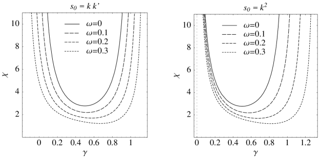
Figure 2: $\chi(\gamma,\omega)$ as a function of $\gamma$ for various values of $\omega$, for the symmetric energy-scale $s_{0}=kk^{\prime}$ on the left and for $s_{0}=k^{2}$ on the right. Here $n_{f}=0$.

In the symmetric energy-scale case, we can see how the original $\gamma$-poles at $\gamma=0,1$ are displaced in a symmetric way for $\omega\neq 0$. The slight asymmetry of $\chi(\gamma,\omega)$ is due to Eq. (3.10), which in turn comes from the perturbative expansion in $\bar{\alpha}_{\mathrm{s}}(t)$, as discussed in Sec. 3.1. Even for sizeable values of $\omega$ the eigenvalue function preserves its shape, with a stable minimum ($\chi^{\prime\prime}(\gamma_{m},\omega)>0$) around $\gamma=1/2$. This stability is a necessary condition to avoid the oscillating behavior noticed in Ref. [27].

With the “upper” scale choice $s_{0}=k^{2}$, the pole at $\gamma=0$ is $\omega$-independent as it should, while the pole at $\gamma=1$ is shifted for $\omega\neq 0$. In this case we also have a stable minimum, in a slightly different position with respect to the previous case ($\gamma_{m}\to\gamma_{m}+\mbox{\small$\frac{1}{2}$}\omega$).

A second way of looking at the resummed kernel is to examine a quantity which we call $\chi_{{\rm eff}}^{(u)}(\gamma,\bar{\alpha}_{\mathrm{s}})$, defined by

$$\chi_{{\rm eff}}^{(u)}(\gamma,\bar{\alpha}_{\mathrm{s}})=\chi^{(u)}(\gamma,\omega=\bar{\alpha}_{\mathrm{s}}\chi_{{\rm eff}}^{(u)})\,.$$ (4.5)

This is closely related to the saddle-point approximation for evaluating the $\gamma$-representation, (2.28), since the value of the saddle-point, $\bar{\gamma}$ satisfies $\omega=\bar{\alpha}_{\mathrm{s}}\chi_{{\rm eff}}^{(u)}(\bar{\gamma},\bar{\alpha}_{\mathrm{s}})$; $\bar{\gamma}$ in such a case is itself closely related to the effective anomalous dimension, (2.31). In Fig. 3 we show

Figure 3: $\chi_{{\rm eff}}^{(u)}(\gamma,\bar{\alpha}_{\mathrm{s}})$ as a function of $\gamma$ for various values of $\bar{\alpha}_{\mathrm{s}}$, for energy-scale $s_{0}=k^{2}$ and $n_{f}=0$.

$\chi_{{\rm eff}}^{(u)}(\gamma,\bar{\alpha}_{\mathrm{s}})$ for different values of $\bar{\alpha}_{\mathrm{s}}$. The marked asymmetry is due to the energy-scale choice $s_{0}=k^{2}$. We note the rather different structure from the $\chi(\gamma,\omega)$ shown in Fig. 2. In particular there are no longer any divergences. That on the right is shifted by an amount $\omega$: as a result rather than a pole one has $\chi_{{\rm eff}}^{(u)}\sim\gamma/\bar{\alpha}_{\mathrm{s}}$, as discussed in [9]. That on the left instead becomes $\chi_{{\rm eff}}^{(u)}\sim\bar{\alpha}_{\mathrm{s}}{\rm e}^{-\gamma/\bar{\alpha}_{\mathrm{s}}}$ for negative $\gamma$ as a result of the inclusion of the dependence on the DGLAP splitting function (in particular the $1/(1-z)$ part, which gives $A_{1}(\omega)\simeq-\log\omega$ for $\omega\to+\infty$). Another feature of $\chi_{{\rm eff}}^{(u)}$ worth noting (though not immediately visible from Fig. 3) is that for $n_{f}=0$, $\bar{\alpha}_{\mathrm{s}}\chi_{{\rm eff}}^{(u)}(0,\bar{\alpha}_{\mathrm{s}})=1$, independently of $\bar{\alpha}_{\mathrm{s}}$. This is so because close to $\gamma=0$

$$\omega=\bar{\alpha}_{\mathrm{s}}\chi_{{\rm eff}}^{(u)}=\bar{\alpha}_{\mathrm{s}}\frac{1+\omega A_{1}(\omega)}{\gamma}+{\mathcal{O}}(\bar{\alpha}_{\mathrm{s}})\,.$$ (4.6)

For $\gamma=0$, we have that $1+\omega A_{1}(\omega)=0$. Since $A_{1}(1)=-1$, $\omega=1$ at $\gamma=0$. This point is of significance insofar as it relates to the problem of ensuring conservation of the momentum sum-rule for the gluon distribution (its $\omega=1$ moment).

Figure 4: $g_{\omega}(t){\rm e}^{-t/2}$ for $\omega=0.15$, with energy-scale $s_{0}=k^{2}$. The normalization is arbitrary.

Next we examine the properties of the regular solution of the small-$x$ equation for the integrated gluon distribution in Eq. (2.28). In order to concentrate on the region most relevant for a consideration of the small-$x$ properties of the anomalous dimension, in Fig. 4 we actually show $g_{\omega}(t){\rm e}^{-t/2}$, as a function of $t=\ln k^{2}/\Lambda^{2}$. There are two critical points on the curve. Firstly the point labelled $\chi^{\prime}(\bar{\gamma})=0$, namely where the saddle-point solution $b\omega t=\chi(\bar{\gamma},\omega)$ sits at the minimum of $\chi$ for that $\omega$. Let us refer to that point as $t_{s}$. The second point of interest, which we call $t_{c}$, is the rightmost zero of $g_{\omega}$. This is the point where the effective anomalous dimension has a divergence. Since the solution in this region has roughly the form [13]

$$g_{\omega}(t)\sim\mathrm{Ai}\left(\left(\frac{2}{\chi_{m}^{\prime\prime}b^{2}\omega^{2}}\right)^{1/3}(b\omega t-\chi_{m})\right).$$ (4.7)

One can estimate the difference between $t_{c}$ and $t_{s}$ as being

$$t_{s}-t_{c}=\xi_{0}\left(\frac{\chi^{\prime\prime}_{m}}{2b\omega}\right)^{1/3}+{\mathcal{O}}\left(1\right)\,,$$ (4.8)

where $-\xi_{0}\simeq-2.3381$ is the position of the rightmost zero of the Airy function. For fixed $\alpha_{\mathrm{s}}$, this translates to a difference between the estimates for $\omega_{s}$ and $\omega_{c}$ which, for $\bar{\alpha}_{\mathrm{s}}\ll 1$, has the following form:

$$\omega_{s}-\omega_{c}=\xi_{0}\left(\frac{b^{2}\chi_{m}^{2}\chi_{m}^{\prime\prime}}{2}\right)^{1/3}\bar{\alpha}_{\mathrm{s}}^{5/3}+{\mathcal{O}}\left(\bar{\alpha}_{\mathrm{s}}^{2}\right)\simeq 11.16\,\bar{\alpha}_{\mathrm{s}}^{5/3}\,.$$ (4.9)

Such $\alpha_{\mathrm{s}}^{5/3}$ contributions to $\omega$ have already been observed in other contexts where there is some form of cutoff on transverse momenta, such as a running coupling which is zero below a certain value of $t$, or non-forward elastic scattering (where the exchanged transverse momentum places an effective cutoff on transverse momenta in the evolution) [14, 35]. Numerical estimates (based on the $\gamma$-representation) for the difference between $\omega_{s}$ and $\omega_{c}$ coincide with (4.9) but only for very small $\bar{\alpha}_{\mathrm{s}}$.

For typical values of $\bar{\alpha}_{\mathrm{s}}$, we note that $\omega_{s}-\omega_{c}\simeq 11.16\bar{\alpha}_{\mathrm{s}}^{5/3}$ is of the same order as the NLL corrections. It too, as pointed out in [14, 35], is the first term of a poorly convergent series. The resummation procedure that we recommend (and adopt) is to define $\omega_{c}$ not through the power series in $\bar{\alpha}_{\mathrm{s}}$, but by looking for the rightmost zero of the regular solution.

4.3 Estimate of error

The question now arises: what is the error that we make in the NL truncation of the RG improved equation? Our claim is that, in the improved formulation, based on the $\omega$-expansion (4.3), this error is smaller than in the formal NL expansion in $\alpha_{\mathrm{s}}(t)$. Let us in fact estimate the remaining terms in Eq. (4.2b). According to Eq. (2.6) further subleading eigenvalue functions contain at least higher order collinear poles which contribute to $\eta_{2}^{\omega}$, $\eta_{3}^{\omega}$ and so on. A first observation is that, even if $\chi_{n}^{\omega}$ has ($n+1$)-th order poles, the $\eta_{n}^{\omega}$’s have at most simple poles, due to the powers of $\chi_{0}^{\omega}$ in the denominator, roughly due to the replacement $\bar{\alpha}_{\mathrm{s}}(t)\sim\omega/\chi_{0}^{\omega}$. Therefore, their contribution cannot be too big, even for small values of $\gamma={\mathcal{O}}(\omega)$.

Furthermore, one can check that, if $q\bar{q}$ contributions (Sec. 4.2) are neglected, the leading collinear poles actually cancel out in the expansions (2.26) of $\eta_{2}^{\omega}$, $\eta_{3}^{\omega}$, …around both $\gamma=0$ and $\gamma=1$. The mechanism of this cancellation can be cleared up as follows.

From the mathematical point of view , it is possible to have the truncated NL solution to be an exact solution of Eq. (2.8), provided the following recurrence relations hold (App. A.2)

$${\chi_{2}^{\omega}\over\chi_{0}^{\omega}}=\left({\chi_{1}^{\omega}\over\chi_{0}^{\omega}}-b\partial_{\gamma}\right){\chi_{1}^{\omega}\over\chi_{0}^{\omega}}\,,\qquad{\chi_{3}^{\omega}\over\chi_{0}^{\omega}}=\left({\chi_{1}^{\omega}\over\chi_{0}^{\omega}}-b\partial_{\gamma}\right){\chi_{2}^{\omega}\over\chi_{0}^{\omega}}\,,\qquad\cdots\,.$$ (4.10)

It is now really simple to check that such relations build up the collinear singularities (2.6), which therefore must cancel out in the subleading corrections $\eta_{2}^{\omega}$, $\eta_{3}^{\omega}$, …. The recurrence relations (4.10) can also be interpreted as DGLAP equations in $\gamma$-space, for the anomalous dimension $\tilde{\gamma}$ in Eq. (2.5).

From a more physical point of view, it is not possible for simple poles to survive in $\eta_{2}^{\omega}$, $\eta_{3}^{\omega}$, …because, when replaced in the saddle point condition (4.4), they would provide $\omega^{2}$, $\omega^{3}$, …corrections to the one-loop anomalous dimensions which cannot possibly be there. In fact, the full anomalous dimension is accounted for by Eqs. (4.3,4.4) as follows

$$b\omega t\simeq{1\over\bar{\gamma}}+{A_{1}(\omega)\over\bar{\gamma}}\quad\Rightarrow\quad\bar{\gamma}=\bar{\alpha}_{\mathrm{s}}\left({1\over\omega}+A_{1}(\omega)\right)\,,$$ (4.11)

where we have taken the small-$\gamma$ limit of the collinear safe eigenvalue function $\chi^{(u)}(\gamma,\omega)$.

We therefore conclude that, in the purely gluonic case, the NL $\omega$-expansion (4.4) takes into account the collinear behavior to all-orders, and that no further resummation is needed. This point is perhaps more easily seen by replacing the NL truncation of Eq. (4.2b) in the saddle point condition (2.20) to yield the equation

$$b\mu t=\chi_{0}^{\omega}+\mu{\chi_{1}^{\omega}\over\chi_{0}^{\omega}}\quad\Rightarrow\quad\mu={\bar{\alpha}_{\mathrm{s}}\chi_{0}^{\omega}\over 1-\bar{\alpha}_{\mathrm{s}}\displaystyle{{\chi_{1}^{\omega}\over\chi_{0}^{\omega}}}}\,.$$ (4.12)

It is apparent from the last version of Eq. (4.12) that we are dealing with an effective eigenvalue function which resums the collinear behavior as a geometric series.

We are finally able to state that the error in the NL truncation (4.2b) is uniformly ${\mathcal{O}}(\omega^{2})$, the neglected coefficient having no $\gamma=0$ nor $\gamma=1$ singularities at all. This error is therefore of the same size as the ambiguity in the definition of $\chi_{1}^{\omega}$ that we have pointed out before. The corresponding error in the saddle point condition (4.4) is a roughly $\gamma$-independent change of scale $\Delta(bt)={\mathcal{O}}(\omega)$, or $\Delta(\alpha_{\mathrm{s}})={\mathcal{O}}(\omega)\alpha_{\mathrm{s}}^{2}$.

4.4 Extension to $q\bar{q}$ contributions

The coefficient kernels $K_{n}^{\omega}$ take up collinear singularities not only from the nonsingular part of the gluon anomalous dimension $\tilde{\gamma}_{gg}$, but also from $q\bar{q}$ states which are coupled to it in the one-loop gluon/quark-sea anomalous dimension matrix

$$\tilde{\gamma}_{ab}(\omega)=\bar{\alpha}_{\mathrm{s}}A_{ab}(\omega)\equiv\gamma_{ab}(\omega)-\delta_{ag}{\bar{\alpha}_{\mathrm{s}}C_{b}\over N_{c}\omega}\,,$$ (4.13)

where $a=(q,g)$ and $C_{a}=(C_{F},C_{A})\equiv N_{c}(r,1)$ denote the partonic channels and color charges.

Although the numerical effect of quark-sea contributions to the gluon anomalous dimensions is pretty small [25], including the two-channel evolution (4.13) changes the collinear problem conceptually. While the small-$x$ equation stays of one-channel type, due to the high-energy gluon exchange, the two-channel collinear behavior yields two anomalous dimension eigenvalues

$$\gamma_{\pm}={\gamma_{gg}+\gamma_{qq}\over 2}\pm\sqrt{\left({\gamma_{gg}-\gamma_{qq}\over 2}\right)^{2}+\gamma_{qg}\gamma_{gq}}\,,$$ (4.14)

with the approximate NL expansions ($\displaystyle{\left[{\gamma_{gq}/\gamma_{gg}}\right]_{\rm Leading}=r}$)

$$\gamma_{+}\simeq\gamma_{gg}+r\gamma_{qg}\,,\qquad\gamma_{-}\simeq\gamma_{qq}-r\gamma_{qg}\,,\qquad\left(r\equiv{C_{F}\over C_{A}}\right)\,.$$ (4.15)

Recovering in the BFKL framework the full collinear behavior (4.14) is not trivial, because $\gamma_{-}\simeq-r\gamma_{qg}^{(1)}={\mathcal{O}}(\alpha_{\mathrm{s}})$ starts at NL level and for $\gamma={\mathcal{O}}(\alpha_{\mathrm{s}})$ the leading $\log s$ hierarchy breaks down in the $\alpha_{\mathrm{s}}$-expansion [25]. What do things look like in the $\omega$-expansion?

Note first that the derivation of the collinear behavior of $K_{n}^{\omega}$ in Sec. 3 can be repeated, by replacing $A_{1}(\omega)$ with the matrix ${\mathbf{A}}(\omega)$ in Eq. (4.13), and by projecting the final results onto the gluon channel, which corresponds to a bracket between initial state ${0\choose 1}$ and final state $(r\;1)$, because the quark couples to the high-energy gluon with relative strength $r=C_{F}/C_{A}$. Therefore, Eq. (2.6) should be replaced by

$$\chi_{n}^{\omega}(\gamma) \simeq{1\over(\gamma+\textstyle{1\over 2}\omega)^{n+1}}\langle(r\;1)|\,1\cdot{\mathbf{A}}\cdot({\mathbf{A}}+b)\cdots({\mathbf{A}}+(n-1)b)\,|{0\choose 1}\rangle\,,\qquad\gamma\ll 1\,,$$ (4.16)

$$\simeq{1\over(1-\gamma+\textstyle{1\over 2}\omega)^{n+1}}\langle(r\;1)|\,1\cdot({\mathbf{A}}-b)\cdots({\mathbf{A}}-nb)\,|{0\choose 1}\rangle\,,\qquad 1-\gamma\ll 1\,.$$

In particular

$$\chi_{1}^{\omega} \simeq{\langle{\mathbf{A}}\rangle\over(\gamma+\textstyle{1\over 2}\omega)^{2}}+{\langle{\mathbf{A}}\rangle-b\over(1-\gamma+\textstyle{1\over 2}\omega)^{2}}\,,$$ (4.17)

$$\chi_{2}^{\omega} \simeq{\langle{\mathbf{A}}({\mathbf{A}}+b)\rangle\over(\gamma+\textstyle{1\over 2}\omega)^{3}}+{\langle({\mathbf{A}}-b)({\mathbf{A}}-2b)\rangle\over(1-\gamma+\textstyle{1\over 2}\omega)^{3}}\,,$$

where $\langle{\mathbf{A}}\rangle=A_{gg}+rA_{qg}$, $\langle{\mathbf{A}}^{2}\rangle$, …denote the brackets defined before in Eq. (4.16).

Secondly, the kernel (3.23) should be supplemented by the ($q\bar{q}$) contribution [32], which completes the $b$-factor in front of the running coupling terms and adds up a collinear contribution, as follows

$$\chi_{1}^{q\bar{q}}(\gamma)= -{1\over 2}\left({-2n_{f}\over 12N_{c}}(\chi_{0}^{2}(\gamma)+\chi_{0}^{\prime}(\gamma))\right)+$$

$$-{n_{f}\over 6N_{c}}\left\{{5\over 3}\chi_{0}(\gamma)+{3\over N_{c}^{2}}\,{\pi^{2}\over\sin^{2}\pi\gamma}\,{\cos\pi\gamma\over 1-2\gamma}\,{1+\textstyle{3\over 2}\gamma(1-\gamma)\over(1+2\gamma)(3-2\gamma)}\right\}\,.$$ (4.18)

Correspondingly, the subtraction term (3.24) changes by the replacement

$$A_{gg}=A_{1}\quad\to\quad\langle{\mathbf{A}}\rangle=A_{gg}+rA_{qg}\,,$$ (4.19)

while $\chi_{0}^{\omega}$ and the subtractions (3.22) and (3.25) are left unchanged.

The main differences with the purely gluonic case come out in the $\omega$-expansion of the solution, and specifically in the role of the higher-order terms. In fact, if we repeat the calculation (4.11) with the new entries (4.17), we find

$$\gamma_{+}^{(1)}=\bar{\alpha}_{\mathrm{s}}\left({1\over\omega}+\langle{\mathbf{A}}\rangle\right)=\bar{\alpha}_{\mathrm{s}}\left({1\over\omega}+A_{gg}(\omega)+rA_{qg}(\omega)\right)\,,$$ (4.20)

which is consistent with the NL expansion (4.15) for $\gamma_{+}$, but is not the full one-loop anomalous dimension (4.14).

Further terms in the $\omega$-expansion must therefore contribute $1/\gamma$ and $1/1-\gamma$ poles, and they indeed do. From Eqs. (2.31) and (4.17) we find

$$\Delta\gamma_{+}^{(1)}=\left(\langle{\mathbf{A}}^{2}\rangle-\langle{\mathbf{A}}\rangle^{2}\right)\bar{\alpha}_{\mathrm{s}}\omega+\langle({\mathbf{A}}-\langle{\mathbf{A}}\rangle)^{3}\rangle\bar{\alpha}_{\mathrm{s}}\omega^{2}+\cdots$$ (4.21)

which checks with the explicit expansion of Eq. (4.14) up to the relevant order. The explicit matrix form of the corrections in Eq. (4.21) makes it clear why the two-channel problem allows the survival of the simple $\gamma$-poles at higher subleading orders.

Nevertheless, the small $\omega$-expansion remains smoother than the $\alpha_{\mathrm{s}}$-expansion. In fact, the ${\mathcal{O}}(\omega^{2})$ NNL terms being neglected show simple poles only (around $\gamma=0,1$), the general trend remains the same as in Fig. 2, provided $\omega$ is not too large. If $\omega$ increases, $\gamma_{+}$ decreases, and at some critical value of $\omega$, for which $\gamma_{+}$ and $\gamma_{-}$ become of the same order, the $\omega$-expansion will break down, eventually. Whether or not the low-energy eigenvalue $\gamma_{-}$ can still be described by an all-order resummation in $\omega$ remains an open question.

5 Anomalous dimension and hard pomeron

Here we present our main numerical results, for both the improved gluon anomalous dimension and the hard pomeron, and we show their stability.

5.1 Results

Figure 5: The anomalous dimension in various approximations

Fig. 5 shows the purely gluonic anomalous dimension as a function of $\omega$ for $\bar{\alpha}_{\mathrm{s}}=0.2$. The LL anomalous dimension is just $\gamma_{LL}=\chi_{0}^{-1}(\omega/\bar{\alpha}_{\mathrm{s}})$ and has the familiar branch-cut at $\omega=4\ln 2\bar{\alpha}_{\mathrm{s}}$. The NLL anomalous dimension is taken as

$$\gamma_{NLL}=\gamma_{LL}-\bar{\alpha}_{\mathrm{s}}\frac{\chi_{1}(\gamma_{LL})}{\chi_{0}^{\prime}(\gamma_{LL})}\,,$$ (5.1)

and has the feature that it is always negative, with a divergent structure around the same point as $\gamma_{LL}$. The resummed result, defined in Eqs. (2.28) and (2.33), shows a divergence at a much lower $\omega$, defined by $\omega_{c}(t)$ in Eq. (2.34). What is particularly remarkable is the similarity to the DGLAP result until very close to the divergence. The momentum sum rule is automatically conserved: for $\omega=1$ we have $\gamma_{{\rm eff}}=0$ (this is closely connected with the fact that $\bar{\alpha}_{\mathrm{s}}\chi_{{\rm eff}}^{(u)}(0)=1$) — in past approaches the need to impose this property in some arbitrary way was a major source of uncertainty [36, 37, 26].

Another interesting feature of the resummed anomalous dimension is that, for small $\bar{\alpha}_{\mathrm{s}}$, the divergence at $\omega_{c}$ is proportional to $\bar{\alpha}_{\mathrm{s}}^{2}$ and not to $\bar{\alpha}_{\mathrm{s}}$:

$$\gamma_{{\rm eff}} =-\frac{1}{\omega-\omega_{c}}\frac{d\omega_{c}}{dt}+{\mathcal{O}}\left(1\right)$$ (5.2a)

$$\simeq\left(\chi_{m}-\frac{5}{3}\left(\frac{b^{2}\chi_{m}^{2}{\chi_{m}}^{\prime\prime}}{2}\right)^{1/3}\xi_{0}\bar{\alpha}_{\mathrm{s}}^{2/3}\right)\frac{b\,\bar{\alpha}_{\mathrm{s}}^{2}}{\omega-\omega_{c}}\,,\qquad\qquad\omega-\omega_{c}\ll 1\,,$$ (5.2b)

which follows from the linear behavior of the regular solution close to the zero, e.g., in the Airy representation of Eq. (4.7). The singularity (5.2) causes the effective splitting function to be power behaved for $x\to 0$, i.e., $P_{{\rm eff}}(x,t)\sim x^{-\omega_{c}(t)}$. Note however that, since $\omega_{c}(t)$ comes from a zero of $g_{\omega}(t)$, the singularity (5.2) does not necessarily transfer to $g_{\omega}(t)$ itself which, according to Eq. (2.28), is expected to have an essential singularity at $\omega=0$ only, even if a complete analysis of possible singularities in the complex $\omega$-plane is still needed.

Figure 6: $\omega_{c}$ and $\omega_{s}$ as a function of $\alpha_{\mathrm{s}}$ for the BFKL kernel with $n_{f}=0$.

The values of the exponents $\omega_{c}$ and $\omega_{s}$ as a function of $\alpha_{\mathrm{s}}$ (and $Q^{2}$), are shown in Fig. 6 and compared with the LL and pure NLL results. It is apparent that the improved equation provides sensible predictions even for sizeable values of $\alpha_{\mathrm{s}}$. A significant difference between the two resummed exponents $\omega_{c}$ and $\omega_{s}$ persists even to low values of $\alpha_{\mathrm{s}}$, largely as a consequence of their differing by a slowly convergent series of non-integer powers of $\alpha_{\mathrm{s}}$, as discussed in section 4.2.

The above difference should not be too confusing. The exponent $\omega_{s}(t)$ signals the breakdown of the formal small-$x$ expansion of the anomalous dimension of Eq. (2.31), due to infinite saddle-point fluctuations, while $\omega_{c}(t)$ tells us the position of the singularity of the resummed anomalous dimension. Their difference arises from their different definitions, not from some instability of our approach (cf. Sec. 5.2).

What is the relation that such quantities bear to the pomeron singularity $\omega_{\mathbb{P}}$, the leading $\omega$-plane singularity of the gluon Green’s function? Though the latter is dependent on the strong coupling region, we expect that $\omega_{\mathbb{P}}\gtrsim\underset{t}{{\rm Max\,}}\omega_{c}(t)$ for a positive definite $\alpha_{\mathrm{s}}(t)$, due to the very definition of $\omega_{c}(t)$ as a zero of the integrated regular solution $g_{\omega}(t)$, to which ${\mathcal{F}}_{\omega}({\boldsymbol{k}})$ is closely related (Sec. 4.2). In fact $\omega_{\mathbb{P}}$ is defined as the value of $\omega$ being itself equal to the endpoint of the spectrum: $\omega_{\mathbb{P}}=\mu_{\mathbb{P}}(\omega_{\mathbb{P}})$ (Sec. 2.3), and thus corresponds to a nodeless ${\mathcal{F}}_{\omega}({\boldsymbol{k}})$, regular for $t\to-\infty$ also. Therefore, if the interaction does not change sign ($\alpha_{\mathrm{s}}(t)>0$), ${\mathcal{F}}_{\omega}({\boldsymbol{k}})$ can have a node for $\omega<\omega_{\mathbb{P}}$ only, so that $\omega_{c}(t)<\omega_{\mathbb{P}}$.

The above remark implies that the small-$x$ behavior of the gluon Green’s function, dominated by the singularity at $\omega=\omega_{\mathbb{P}}$ in $\tilde{{\mathcal{F}}}_{\omega}({\boldsymbol{k}}_{0})$, is not sensitive to the region $\omega\simeq\omega_{c}(t)$ where ${\mathcal{F}}_{\omega}({\boldsymbol{k}})$ changes sign. This fact is consistent with the positivity constraint on the total cross section.

Furthermore, we can state that the frozen $\alpha_{\mathrm{s}}$ regularization of Sec. 2.3 maximizes the interaction strength in the strong coupling region $t\lesssim\bar{t}$, compared to various cut-off procedures. Therefore we also expect $\omega_{\mathbb{P}}<\omega_{s}(\bar{t})$, the value quoted in Eq. (2.18) at the freezing point. It follows that $\underset{t}{{\rm Max\,}}\omega_{c}(t)\lesssim\omega_{\mathbb{P}}\lesssim\underset{t}{{\rm Max\,}}\omega_{s}(t)$ or, in other words, that the two exponents of Fig. 6 provide, in the strong coupling region, lower and upper bounds on the pomeron intercept $\omega_{\mathbb{P}}$. Of course, the precise value of the latter will be dependent on the size and shape of the effective coupling in the small-$k$ region.

5.2 Stability

The original $\mbox{LL}+\mbox{NLL}$ formalism suffered from considerable instabilities under renormalization group scale and scheme changes.

An important characteristic of any resummed approach is that it should be relatively insensitive to such changes, and generally stable. In the approach advocated here, it has already been shown in the previous sections that the formal truncation error is small. It still remains to demonstrate its stability in practice.

Renormalization scale and scheme.

Note first that in our approach the renormalization scale only enters through the RG invariant $\Lambda$ parameter (Eqs. (2.2) and (2.28)). It is then easy to see that the physical results are $\Lambda$-independent. A redefinition of $\Lambda$ is essentially a shift in $t$, say by an amount $\Delta t$. There is a corresponding modification of $\chi_{1}^{\omega}$, $\chi_{2}^{\omega}$, …by the amounts

$$\chi_{1}^{\omega}\to\chi_{1}^{\omega}+b\Delta t\chi_{0}^{\omega}\,,\qquad\chi_{2}^{\omega}\to\chi_{2}^{\omega}+2b\Delta t\chi_{1}^{\omega}+b^{2}(\Delta t)^{2}\chi_{0}^{\omega}\,,\qquad\dots$$ (5.3)

In the off-shell $\gamma$-representation (4.2b), this corresponds to a modification of $X_{\omega}$ by an amount $b\mu\gamma\Delta t$. In fact the transformation (5.3) changes the coefficient $\eta_{1}$ only, the remaining ones $\eta_{2}$, $\eta_{3}$,…being left invariant. This change exactly cancels the modification of $t$ itself:

$$\exp\left\{\gamma t-{1\over b\mu}X_{\omega}(\gamma,\mu)\right\}\to\exp\left\{\gamma(t+\Delta t)-{1\over b\mu}(X_{\omega}(\gamma,\mu)+b\mu\gamma\Delta t)\right\}\,,$$ (5.4)

thus implying that the physical results are independent of the $\Lambda$-parameter choice. This automatic resummation of the renormalization scale alleviates the need for techniques such as BLM resummation [33], advocated for example in [34], which show a strong renormalization scheme dependence.

The issue of renormalization scheme dependence is in fact closely related. Consider a scheme $S$ related to the $\overline{MS}$ scheme by

$$\alpha_{\mathrm{s}}^{(S)}=\alpha_{\mathrm{s}}^{(\overline{\mbox{\scriptsize MS}})}+T\alpha_{\mathrm{s}}^{2}\,,$$ (5.5)

with an appropriate modification of $\chi_{1}^{\omega}$. Except for terms of ${\mathcal{O}}\left(\alpha_{\mathrm{s}}^{3}\right)$ and higher, this is identical to a renormalization scale change. Indeed if one defines the scheme change by a modification of $\Lambda$ then renormalization scheme changes behave exactly as renormalization scale changes, and so have no effect on the answer. Using instead (5.5) there is some residual dependence on the scheme at ${\mathcal{O}}\left(\alpha_{\mathrm{s}}^{3}\right)$, but as one can see in Fig. 7 for the $\Upsilon$ scheme, which has $T\simeq 1.17$ (for $n_{f}=0$), the effect of the change of scheme is small.

Figure 7: Renormalization scheme uncertainty of the two exponents; $\overline{MS}$ scheme and $\Upsilon$ scheme; $\alpha_{\mathrm{s}}$ is always shown in the $\overline{MS}$ scheme, and is connected to the $\Upsilon$ scheme value of $\alpha_{\mathrm{s}}$ via (5.5).

Resummation scheme.

In resumming the double transverse logarithms (energy-scale terms), there is some freedom in one’s choice of how to shift the poles around $\gamma=0$ and $\gamma=1$. In a similar manner to what was done in [9] we consider two choices. The one explicitly discussed in this paper (and the one used for all the figures elsewhere in this paper) can be summarized as

$$\psi^{(n-1)}(\gamma)\to\psi^{(n-1)}(\gamma+\mbox{\small$\frac{1}{2}$}\omega)\,,$$ (5.6)

with an equivalent procedure around $\gamma=1$. We refer to this as resummation type (a). An alternative possibility is

$$\frac{1}{\gamma^{n}}\to\frac{1}{(\gamma+\mbox{\small$\frac{1}{2}$}\omega)^{n}}\,.$$ (5.7)

Thus we have

$$\chi_{0}^{\omega}(\gamma) =\chi_{0}(\gamma)-\frac{1}{\gamma}-\frac{1}{1-\gamma}+\frac{1}{\gamma+\mbox{\small$\frac{1}{2}$}\omega}+\frac{1}{1-\gamma+\mbox{\small$\frac{1}{2}$}\omega}\,,$$ (5.8a)

$$\chi_{1}^{\omega}(\gamma) =\tilde{\chi}_{1}(\gamma)+\frac{A_{1}(\omega)}{(\gamma+\mbox{\small$\frac{1}{2}$}\omega)^{2}}+\frac{A_{1}(\omega)-b}{(1-\gamma+\mbox{\small$\frac{1}{2}$}\omega)^{2}}+\displaystyle\frac{1}{2}\left(\frac{1}{\gamma+\mbox{\small$\frac{1}{2}$}\omega}+\frac{1}{1-\gamma+\mbox{\small$\frac{1}{2}$}\omega}\right)\,,$$ (5.8b)

$$\tilde{\chi}_{1}(\gamma) =\chi_{1}(\gamma)+{\chi_{0}(\gamma)\over 2}\left(\frac{1}{\gamma^{2}}+\frac{1}{(1-\gamma)^{2}}\right)-{1\over 2}\left(\frac{1}{\gamma}+\frac{1}{1-\gamma}\right)-\frac{A_{1}(0)}{\gamma^{2}}-\frac{A_{1}(0)-b}{(1-\gamma)^{2}}\,.$$ (5.8c)

A comparison of these two resummation schemes is given in Fig. 8 and the difference between them is again reasonably small.

Figure 8: Resummation scheme uncertainty of the two exponents.

Aside from the explicit renormalization-scale independence, the stability of our approach is connected with the resummation of the collinear poles, for both the double-log, energy-scale dependent terms (the $1/\gamma^{3}$ and $1/(1-\gamma)^{3}$ poles at NLO) and for the single-log ones of Eqs. (4.11) and (4.12). Stability has been noted elsewhere, in the study of a rapidity veto (initially examined in [38]) combined with a resummation of the energy-scale terms [39].

6 Conclusions

In this paper, we have improved the small-$x$ equation in several ways. Firstly, we have taken into account the collinear limits, and their scale dependence. This implies the $\omega$-shifts of the $\gamma$-singularities in Eq. (2.6), which yield a double-log resummation of parameters like $\omega/\gamma\simeq\alpha_{\mathrm{s}}/\gamma^{2}$ or $\omega/1-\gamma$, and implies also the effective characteristic function in Eq. (4.12), which yields a single-log resummation in the parameter $\alpha_{\mathrm{s}}\chi_{1}/\chi_{0}\simeq\alpha_{\mathrm{s}}/\gamma$ or $\alpha_{\mathrm{s}}/1-\gamma$.

Both kinds of resummation require an infinite number of subleading terms in the original BFKL formalism, in which both $\omega$ and the running coupling play the role of expansion parameters. The RG improved kernel (Eq. (2.2)) is actually an infinite series in $\alpha_{\mathrm{s}}(t)$ of $\omega$-dependent kernels, so that the corresponding Eq. (2.8) is no longer an evolution equation in $\log 1/x$ with a simple dependence on the conjugate variable $\omega$, but a much more general $\omega$-dependent integral equation.

The second important improvement concerns the treatment of this generalized equation. In the limit in which the Green’s function is factorized (Eq. (2.7)) we have singled out the solutions of the homogeneous equation ${\mathcal{F}}_{\omega}({\boldsymbol{k}})$ ($\tilde{{\mathcal{F}}}_{\omega}({\boldsymbol{k}}_{0})$) which are regular for $t\to+\infty$ ($t\to-\infty$), and we have provided a general method for the construction of ${\mathcal{F}}_{\omega}({\boldsymbol{k}})$ in Eq. (2.19). The latter exploits $\omega$ as expansion parameter (or the eigenvalue $\mu\neq\omega$ if referred to the eigenfunctions (2.11)), and thus we call it $\omega$-expansion. It allows the construction, in terms of the improved kernels, of the characteristic function $\chi(\gamma,\omega)$ of Eqs. (4.2b) and (4.4), which shows no sign of instability when $\omega$ increases (Fig. 2), even if the improved kernel is truncated at NL accuracy.

The key advantages of the improved equation concern the calculation of the $t$-dependence, or of the resummed anomalous dimensions, which can be given in terms of ${\mathcal{F}}_{\omega}({\boldsymbol{k}})$ only. Let us list some of them:

• The resummation involves not only all powers of $\alpha_{\mathrm{s}}/\omega$, but also an infinite number of subleading terms and extrapolates quite smoothly the fixed order perturbative result (Fig. 5).

• Although we resum only a fraction of such subleading terms, we have characterized the error that we make as a constant scale change $\Delta t={\mathcal{O}}(\omega)$, or $\Delta\alpha_{\mathrm{s}}/\alpha_{\mathrm{s}}={\mathcal{O}}(\alpha_{\mathrm{s}}\,\omega)$. Therefore, the neglected terms are subleading, order by order, in both $\alpha_{\mathrm{s}}/\omega$ and $\alpha_{\mathrm{s}}$ expansions.

• Although we are limited in principle to small $\omega$’s, we incorporate exact one-loop (and partly two-loop) anomalous dimensions in the $\omega$-dependent kernels. In particular, we have exact energy-momentum conservation, i.e., the gluon anomalous dimension vanishes for $\omega=1$.

We have provided two critical exponents $\omega_{s}(t)$ and $\omega_{c}(t)$ that signal the breakdown of the above resummation. The first one ($\omega_{s}(t)$) is roughly related to the breakdown of the $\alpha_{\mathrm{s}}/\omega$ resummation, or better of the saddle point (“semiclassical”) approximation, valid for large $b\omega t$ (or $\alpha_{\mathrm{s}}/\omega\ll 1$), and was the only one considered in previous L+NL estimates. The latter exponent ($\omega_{c}(t)$) comes from a zero of the gluon density and signals a singularity of the resummed anomalous dimension series. Their difference involves non-integer powers of $\alpha_{\mathrm{s}}$ ($\alpha_{\mathrm{s}}^{5/3}$ and higher) which are related to a “quantum” wavelength in the $t$-dependence.

The estimates of $\omega_{s}(t)$ and $\omega_{c}(t)$ (Fig. 6) in the improved formulation are now quite stable (Figs. 7 and 8) — despite the large size of NL corrections — and nearly renormalization-scheme independent! The reason for that stems from both the collinear improvement of the kernel, and from the RG invariant formulation of the solution. Both exponents are actually useful for a full understanding of the solution $\tilde{{\mathcal{F}}}_{\omega}({\boldsymbol{k}}_{0})$, carrying the (non-perturbative) pomeron singularity $\omega_{\mathbb{P}}$. Indeed we have argued that — for reasonable strong coupling extrapolations (positive definite $\alpha_{\mathrm{s}}(t)$) — the pomeron intercept is bounded between $\underset{t}{{\rm Max\,}}\omega_{c}(t)$ and $\underset{t}{{\rm Max\,}}\omega_{s}(t)$. Present estimates of the latter (Fig. 6) are consistent with the small-$x$ exponent $\simeq 0.2$ seen for moderate $Q^{2}$ at HERA [40]. But a detailed analysis, including two-scale processes [41, 42], is required to obtain a clearcut picture.

Having no problems with stability, we are now more confident of future progress. We have already mentioned the need for evaluating $\tilde{{\mathcal{F}}}_{\omega}({\boldsymbol{k}})$, the regular solution for $t\to-\infty$, which is much more dependent on the strong coupling region. But also the full Green’s function ${\mathcal{G}}_{\omega}({\boldsymbol{k}},{\boldsymbol{k}}_{0})$ for $k/k_{0}={\mathcal{O}}(1)$ — i.e., outside the the factorization regime — is interesting for the description of two-scale processes (double DIS [41], forward jet [42], etc.). We hope to have a better understanding of both quantities from a simple model with collinear resummation [23].

Of course, a complete understanding involves a variety of other questions, like a realistic evaluation of $\omega_{\mathbb{P}}$, a full inclusion of quarks (Sec. 4.4) and impact factors [22, 43], the relation to the CCFM equation [5, 6] and other two-channel formulations [7], and so on. But we think that, despite some residual uncertainties, we are on the right track.

Acknowledgments

We wish to thank Yuri Dokshitzer, Jeffrey Forshaw, Peter Landshoff, Pino Marchesini, Douglas Ross and Robert Thorne for helpful discussions.

Appendix A $\mu$-Expansion

A.1 Saddle-point method

In this appendix we want to show the saddle point procedure for deriving the dependence of the coefficients $\eta_{j}^{\omega}:j=0,1,\dots$ of the small-$\mu$ expansion for $\chi_{\omega}(\gamma,\mu)$

$$\chi_{\omega}(\gamma,\mu)=\eta^{\omega}_{0}(\gamma)+\mu\,\eta_{1}^{\omega}(\gamma)+\mu^{2}\,\eta_{2}^{\omega}(\gamma)+\cdots\,,$$ (A.1)

in terms of the eigenvalue functions $\chi^{\omega}_{j}:j=0,1,\dots$ of the coefficient kernels in Eq. (1.4).

The action of the improved kernel on its eigenfunctions is

$$0=[{\mathcal{K}}_{\omega}-\mu]{\mathcal{F}}_{\omega}^{\mu}({\boldsymbol{k}})={\bar{\alpha}_{\mathrm{s}}(t)\over{\boldsymbol{k}}^{2}}\int{{\rm d}\gamma\over 2\pi{\rm i}}{\rm e}^{\gamma t-{1\over b\mu}X_{\omega}(\gamma,\mu)}\left[\sum_{n=0}^{\infty}\bar{\alpha}_{\mathrm{s}}(t)^{n}\chi_{n}^{\omega}(\gamma)-b\mu t\right]$$ (A.2)

Now we assume the above integral to be dominated by a saddle point at $\gamma=\bar{\gamma}_{\omega}(\mu,t)$ where $b\mu t=\chi_{\omega}(\gamma,\mu)$, $\chi_{\omega}$ being the $\gamma$-derivative of $X_{\omega}$ (see Eq. (2.20)). By adopting $\bar{\gamma}$ and $\mu$ as independent variables, we replace

$$\bar{\alpha}_{\mathrm{s}}(t)={1\over bt}={\mu\over\chi_{\omega}(\bar{\gamma},\mu)}\,.$$ (A.3)

Introducing the “mean value”

$$\langle A(\gamma)\rangle \equiv{\int A(\gamma){\rm e}^{-V_{\omega}(\gamma,\mu)}\;{\rm d}\gamma\over\int{\rm e}^{-V_{\omega}(\gamma,\mu)}\;{\rm d}\gamma}\,,$$ (A.4)

$$-V_{\omega}(\gamma,\mu) \equiv\left[\gamma t-{1\over b\mu}X_{\omega}(\gamma,\mu)\right]-[\gamma\to\bar{\gamma}]=-{1\over b\mu}\sum_{m=2}^{\infty}{1\over m!}\;\chi^{(m-1)}_{\omega}(\bar{\gamma},\mu)\,\Delta^{m}\,,$$ (A.5)

where ${\displaystyle\chi^{(m)}_{\omega}}\equiv\partial_{\gamma}^{m}\chi_{\omega}$ and $\Delta\equiv\gamma-\bar{\gamma}$, we write Eq. (A.2) in the form

$$\chi_{\omega}(\bar{\gamma},\mu)=b\mu t=\sum_{n=0}^{\infty}\left[{\mu\over\chi(\bar{\gamma},\mu)}\right]^{n}\langle\chi_{n}(\gamma)\rangle\,,$$ (A.6)

having dropped the $\omega$ dependence. We observe that

$$0 =\left(\lim_{\gamma\to+{\rm i}\infty}-\lim_{\gamma\to-{\rm i}\infty}\right){\rm e}^{-V}=\int{\rm d}\gamma\;\partial_{\gamma}\left({\rm e}^{-V}\right)\propto\langle\partial_{\gamma}V\rangle={1\over b\mu}\big{[}\langle\chi(\gamma,\mu)\rangle-b\mu t\big{]}\,.$$ (A.7)

Collecting Eqs. (A.2), (A.6) and (A.7) we obtain the basic equation

$$\langle\chi(\gamma,\mu)\rangle=\sum_{j=0}^{\infty}\mu^{j}\langle\eta_{j}(\gamma)\rangle=\sum_{n=0}^{\infty}\left[{\mu\over\chi(\bar{\gamma},\mu)}\right]^{n}\langle\chi_{n}(\gamma)\rangle\,.$$ (A.8)

At lowest order (${\mathcal{O}}(\mu^{0})$) we have

$$\langle\eta_{0}(\gamma)\rangle=\langle\chi_{0}(\gamma)\rangle\,.$$ (A.9)

One can easily check that $\langle\Delta^{n}\rangle={\mathcal{O}}(\mu^{\left[{n+1\over 2}\right]})$. Since

$$\langle A(\gamma)\rangle=\langle A(\bar{\gamma})\rangle+\langle A^{\prime}(\bar{\gamma})\,\Delta\rangle+\cdots=A(\bar{\gamma})+{\mathcal{O}}(\mu)$$ (A.10)

it follows that, for all $\bar{\gamma}$, $\eta_{0}(\bar{\gamma})=\chi_{0}(\bar{\gamma})$ and hence $\eta_{0}=\chi_{0}$. Taking into account Eq. (A.9), we can simplify Eq. (A.8) as

$$\sum_{j=1}^{\infty}\mu^{j-1}\langle\eta_{j}(\gamma)\rangle=\sum_{n=1}^{\infty}{\mu^{n-1}\over[\chi(\bar{\gamma},\mu)]^{n}}\langle\chi_{n}(\gamma)\rangle\,.$$ (A.11)

The lowest order of this new relation yields

$$\langle\eta_{1}(\gamma)\rangle={\langle\chi_{1}(\gamma)\rangle\over\chi(\bar{\gamma},\mu)}={\chi_{1}(\bar{\gamma})\over\eta_{0}(\bar{\gamma})}+{\mathcal{O}}(\mu)={\chi_{1}(\bar{\gamma})\over\chi_{0}(\bar{\gamma})}+{\mathcal{O}}(\mu)$$ (A.12)

and hence $\eta_{1}=\chi_{1}/\chi_{0}$. The next order reads

$$\langle\eta_{1}(\gamma)\rangle+\mu\langle\eta_{2}(\gamma)\rangle={\langle\chi_{1}(\gamma)\rangle\over\chi(\bar{\gamma},\mu)}+\mu\,{\langle\chi_{2}(\gamma)\rangle\over[\chi(\bar{\gamma},\mu)]^{2}}\,.$$ (A.13)

By expanding with respect to $\gamma$ around $\bar{\gamma}$ yields

$$\eta_{1}(\bar{\gamma}) +\eta^{\prime}_{1}(\bar{\gamma})\langle\Delta\rangle+{1\over 2}\eta^{\prime\prime}_{1}(\bar{\gamma})\langle\Delta^{2}\rangle+\mu\,\eta_{2}(\bar{\gamma})=$$

$$={1\over\chi(\bar{\gamma},\mu)}\left[\chi_{1}(\bar{\gamma})+\chi^{\prime}_{1}(\bar{\gamma})\langle\Delta\rangle+{1\over 2}\chi^{\prime\prime}_{1}(\bar{\gamma})\langle\Delta^{2}\rangle\right]+\mu\,{\chi_{2}(\bar{\gamma})\over[\chi(\bar{\gamma},\mu)]^{2}}\,.$$ (A.14)

To the relevant order in $\mu$, we have

$$\langle\Delta\rangle=-{b\mu\over 2}\,{\chi^{\prime\prime}_{0}(\bar{\gamma})\over[\chi^{\prime}_{0}(\bar{\gamma})]^{2}}\,,\qquad\langle\Delta^{2}\rangle={b\mu\over\chi^{\prime}_{0}(\bar{\gamma})}\,,\qquad{1\over\chi(\gamma,\mu)}={1\over\chi_{0}(\bar{\gamma})}\left(1-\mu\,{\eta_{1}(\bar{\gamma})\over\chi_{0}(\bar{\gamma})}\right)\,,$$ (A.15)

and substituting in Eq. (A.14) we get

$$\left(\eta_{2}-{\chi_{2}\over\chi_{0}^{2}}+{\eta_{1}^{2}\over\chi_{0}}\right) =-{\chi^{\prime}_{0}\chi_{1}\over\chi_{0}^{2}}{b\mu\over 2}{\chi^{\prime\prime}_{0}\over[\chi^{\prime}_{0}]^{2}}+{b\mu\over 2\chi^{\prime}_{0}}\left({\chi^{\prime\prime}_{0}\chi_{1}\over\chi_{0}^{2}}+2{\chi^{\prime}_{0}\chi_{1}\over\chi_{0}^{2}}-2{[\chi^{\prime}_{0}]^{2}\chi_{1}\over\chi_{0}^{3}}\right)$$

$$={b\over\chi_{0}}\,\eta^{\prime}_{1}\,,$$

i.e.,

$$\eta_{2}={1\over\chi_{0}}\left[{\chi_{2}\over\chi_{0}}-(\eta_{1}-b\partial_{\gamma})\eta_{1}\right]\,.$$ (A.16)

Going further requires taking into account higher order terms both in the fluctuations $\langle\Delta^{m}\rangle$ and in the $\mu$-expansion of Eq. (A.11).

The advantage of this method is that it is clearly local in $t$ (because the saddle point $\bar{\gamma}_{\omega}$ is a function of $t$) and in $\gamma$ (because of the finite fluctuations). Therefore, if $t$ is large enough for a stable saddle point to exist, then the procedure and the result are independent of the regularization procedure in the strong coupling region $t\simeq 0$.

The disadvantage, though, is that the order of fluctuations required increases rapidly with the $\mu$-exponent. It turns out in fact that, in order to determine $\eta_{j}:j>2$ — i.e., to evaluate Eq. (A.11) to order $\mu^{j-1}$ —, the most involved calculation concerns $\langle\Delta\rangle$ which requires the computation of the fluctuations in $\int\Delta\,{\rm e}^{-V}\,{\rm d}\gamma$ up to order $6j-8$.

A.2 $\gamma$-Derivative method

By comparison, the $\gamma$-derivative method is formally much simpler. We start rewriting the basic equation (2.24) by introducing the notation

$$\chi_{\omega}(\gamma,\mu)-\chi_{0}(\gamma)\equiv\mu\,\eta_{\omega}(\gamma,\mu)\,,\qquad\eta_{\omega}(\gamma,\mu)=\eta_{1}^{\omega}(\gamma)+\mu\,\eta_{2}^{\omega}(\gamma)+\mu^{2}\,\eta_{3}^{\omega}(\gamma)+\cdots\,,$$

$$D\equiv(\eta_{\omega}-b\,\partial_{\gamma})$$ (A.17)

in the form

$$\eta_{\omega}(\gamma,\mu) =\left[\chi_{0}^{\omega}+\mu D\right]^{-1}\chi_{1}^{\omega}+\left[\chi_{0}^{\omega}+\mu D\right]^{-2}\mu\,\chi_{2}^{\omega}+\cdots$$

$$=\left(1+{\mu\over\chi_{\omega}}\,D\right)^{-1}\left({\chi_{1}^{\omega}\over\chi_{0}^{\omega}}+\chi_{0}^{\omega}{}^{-1}\left(1+{\mu\over\chi_{\omega}}\,D\right)^{-1}\mu{\chi_{2}^{\omega}\over\chi_{0}^{\omega}}+\cdots\right)\,.$$ (A.18)

We then expand in $\mu$ both the $\chi_{n}^{\omega}$ series and the operator denominators, which depend on $\eta_{\omega}$ in a non-linear way, and we derive the $\mu$-expansion (2.25).

For instance, if we want $\eta_{3}^{\omega}$, we can rewrite Eq. (A.18) up to order $\mu^{2}$ in the form

$$\eta =\left(1-\mu\,\chi_{0}^{-1}D+\mu^{2}(\chi_{0}^{-1}D)^{2}\right){\chi_{1}\over\chi_{0}}+{1\over\chi_{0}}\left(1-\mu(D\chi_{0}^{-1}+\chi_{0}^{-1}D)\right)\mu{\chi_{2}\over\chi_{0}}+\mu^{2}{\chi_{3}\over\chi_{0}}$$

$$D =D_{1}+\mu\,\eta_{2}+\cdots\,,\qquad D_{1}\equiv\eta_{1}-b\,\partial_{\gamma}\,,$$ (A.19)

where the $\omega$ index has been dropped.

We then identify the $\eta_{i}$ coefficients in Eq. (A.19) term by term:

$$\eta_{1} ={\displaystyle\chi_{1}\over\chi_{0}}\,,\qquad\eta_{2}={1\over\chi_{0}}\left({\chi_{2}\over\chi_{0}}-D_{1}{\chi_{1}\over\chi_{0}}\right)\,,$$ (A.20)

$$\eta_{3} ={\chi_{3}\over\chi_{0}}-{1\over\chi_{0}}\left(D_{1}{1\over\chi_{0}}+{1\over\chi_{0}}D_{1}\right){\chi_{2}\over\chi_{0}}+\left({1\over\chi_{0}}D_{1}\right)^{2}{\chi_{1}\over\chi_{0}}-{1\over\chi_{0}}\eta_{2}{\chi_{1}\over\chi_{0}}\,,$$

Eq. (A.20) proves Eq. (2.26) of the text.

We notice the curious fact that if

$${\chi_{2}\over\chi_{0}}=D_{1}{\chi_{1}\over\chi_{0}}\,,\qquad{\chi_{3}\over\chi_{0}}=D_{1}^{2}{\chi_{1}\over\chi_{0}}\,,$$ (A.21)

both $\eta_{2}$ and $\eta_{3}$ vanish identically. This is a particular case of Eq. (4.10), which states that $\eta_{1}=\chi_{1}/\chi_{0}$ is an exact solution of Eq. (A.18) if

$${\chi_{n+1}\over\chi_{0}}=D_{1}^{n}{\chi_{1}\over\chi_{0}}\,,\qquad n\geq 1\,.$$ (A.22)

In fact we have the chain of identities

$${\chi_{1}\over\chi_{0}} =\sum_{n=0}^{\infty}\left[(\chi_{0}+\mu D_{1})^{-n}(\mu D_{1})^{n}-(\chi_{0}+\mu D_{1})^{-(n+1)}(\mu D_{1})^{n+1}\right]{\chi_{1}\over\chi_{0}}$$ (A.23)

$$=\sum_{n=0}^{\infty}(\chi_{0}+\mu D_{1})^{-(n+1)}\chi_{0}(\mu D_{1})^{n}{\chi_{1}\over\chi_{0}}=\sum_{n=0}^{\infty}(\chi_{0}+\mu D_{1})^{-(n+1)}\chi_{n+1}\,,$$ (A.24)

which prove Eq. (A.18) if Eq. (A.22) is satisfied.

It is straightforward to check that the ansatz (A.22) builds up the correct collinear singularities to all orders. We start from

$${\chi_{1}\over\chi_{0}}\simeq{A_{1}\over\gamma}\quad,\quad{A_{1}-b\over 1-\gamma}\qquad(\gamma\to 0,1)$$ (A.25)

and, by applying the $D_{1}$ operator of Eq. (A.22) in the relevant limits we obtain the result

$${\chi_{n+1}\over\chi_{0}}\simeq\left({A_{1}\over\gamma}-b\,\partial_{\gamma}\right)^{n}{A_{1}\over\gamma}\quad,\quad\left({A_{1}-b\over 1-\gamma}-b\,\partial_{\gamma}\right)^{n}{A_{1}-b\over 1-\gamma}\,,$$ (A.26)

which checks with Eq. (2.6). It follows that the leading collinear singularities must cancel out in $\eta_{j}:j\geq 2$, as stated in Sec. 4.3.

We should keep in mind that the two methods just illustrated are equivalent when both make sense, i.e., for $t$ large enough for the stable saddle point to exist. This assumption is implicitly present in the $\gamma$-derivative method when we expand the operators in Eq. (A.18). This means that we stay away from the zero modes of the full operator and we consider the $D$ operator as a small perturbation with respect to $\chi_{0}$. Expanding in $D$ is analogous to the fluctuation expansion.

References

• [1] V.S. Fadin and L.N. Lipatov, Phys. Lett. 429B (1998) 127 and references therein.
• [2] G. Camici and M. Ciafaloni, Phys. Lett. 412B (1997) 396;
G. Camici and M. Ciafaloni, Phys. Lett. 430B (1998) 349.
• [3] E.A. Kuraev, L.N. Lipatov and V.S. Fadin, Sov. Phys. JETP 45 (1978) 199;
Y.Y. Balitski and L.N. Lipatov, Sov. J. Nucl. Phys. 28 (1978) 22.
• [4] V.N. Gribov and L.N. Lipatov, Sov. J. Nucl. Phys. 15 (1972) 438;
G. Altarelli and G. Parisi, Nucl. Phys. B126 (1977) 298;
Y.L. Dokshitzer, Sov. Phys. JETP 46 (1977) 641.
• [5] M. Ciafaloni, Nucl. Phys. B296 (1988) 49.
• [6] S. Catani, F. Fiorani and G. Marchesini, Phys. Lett. 234B (1990) 339;
S. Catani, F. Fiorani and G. Marchesini, Nucl. Phys. B336 (1990) 18.
• [7] J. Kwiecinski, A.D. Martin and A.M. Stasto, Phys. Rev. D56 (1997) 3991; see also
M. Krawczyk, Nucl. Phys. Proc. Suppl. 18C (1991) 64.
• [8] M. Ciafaloni and D. Colferai, Phys. Lett. 452B (1999) 372.
• [9] G.P. Salam, JHEP 9807 (1998) 19.
• [10] J. Kwiecinski, Zeit. Phys. C29 (1985) 561;
J.C. Collins and J. Kwiecinski, Nucl. Phys. B316 (1989) 307.
• [11] G. Camici and M. Ciafaloni, Phys. Lett. 395B (1997) 118.
• [12] L.V. Gribov, E.M. Levin and M.G. Ryskin, Phys. Rep. 100 (1983) 1.
• [13] L.N. Lipatov, Sov. Phys. JETP 63 (1986) 904.
• [14] R.E. Hancock and D.A. Ross, Nucl. Phys. B383 (1992) 575;
R.E. Hancock and D.A. Ross, Nucl. Phys. B394 (1993) 200.
• [15] N.N. Nikolaev and B.G. Zakharov, Phys. Lett. 327B (1994) 157.
• [16] E.M. Levin, Nucl. Phys. B453 (1995) 303.
• [17] M.A. Braun, Phys. Lett. 345B (1995) 155.
• [18] L.P.A. Haakman, O.V. Kancheli and J.H. Koch, Phys. Lett. 391B (1997) 157;
L.P.A. Haakman, O.V. Kancheli and J.H. Koch, Nucl. Phys. B518 (1998) 275.
• [19] Y.V. Kovchegov and A.H. Mueller, Phys. Lett. 439B (1998) 428.
• [20] J. Bartels, Nucl. Phys. B175 (1980) 365;
J. Kwiecinski and M. Praszalowicz, Phys. Lett. 94B (1980) 413;
L.N. Lipatov, Sov. Phys. JETP 59 (1994) 571;
A.H. Mueller, Nucl. Phys. B437 (1995) 107.
• [21] M. Ciafaloni, Phys. Lett. 429B (1998) 363.
• [22] M. Ciafaloni and D. Colferai, Nucl. Phys. B538 (1999) 187.
• [23] M. Ciafaloni, D. Colferai and G.P. Salam, to appear.
• [24] Y.L. Dokshitzer, G. Marchesini and B.R. Webber, Nucl. Phys. B469 (1996) 93.
• [25] G. Camici and M. Ciafaloni, Nucl. Phys. B496 (1997) 305.
• [26] J. Blümlein and A. Vogt, Phys. Rev. D58 (1998) 014020.
• [27] D.A. Ross, Phys. Lett. 431B (1998) 161;
E.M. Levin, hep-ph/9806228.
• [28] R.S. Thorne, hep-ph/9901331.
• [29] B. Andersson, G. Gustafson and J. Samuelsson, Nucl. Phys. B467 (1996) 443.
• [30] M. Ciafaloni, Communication at the Durham workshop (1998).
• [31] M. Toller, Nuovo Cimento 37 n.2 (1965) 631.
• [32] G. Camici and M. Ciafaloni, Phys. Lett. 386B (1996) 341.
• [33] S.J. Brodsky, G.P. Lepage and P.N. Mackenzie, Phys. Rev. D28 (1983) 228.
• [34] S.J. Brodsky, V.S. Fadin, V.T. Kim, L.N. Lipatov and G.B. Pivovarov, hep-ph/9901229.
• [35] J.R. Forshaw and D.A. Ross, Perturbative QCD and the Pomeron, Cambridge University Press, 1997.
• [36] R.K. Ellis, F. Hautmann and B. R. Webber, Phys. Lett. 348B (1995) 582.
• [37] R.D. Ball and S. Forte, Proceedings of the DIS 96 Workshop, 1996.
• [38] C. Schmidt, preprint MSUHEP-90122, hep-ph/9901397.
• [39] J.R. Forshaw, D.A. Ross and A. Sabio Vera, preprint CERN-TH/99-64, MC-TH-99-04, SHEP -99/02, hep-ph/9903390.
• [40] H1 Collaboration (Adloff et al.), Zeit. Phys. C72 (1996) 593;
ZEUS Collaboration (Breitweg et al.), Phys. Lett. 407B (1997) 402.
• [41] L3 Collaboration (M. Acciarri et al.), Phys. Lett. 453B (1999) 333.
• [42] ZEUS Collaboration (J. Breitweg et al.), Eur. Phys. J. C6 (1999) 239;
H1 Collaboration (C. Adloff et al.), Nucl. Phys. B538 (1999) 3.
• [43] S.J. Brodsky, F. Hautmann and D.E. Soper, Phys. Rev. D56 (1997) 6957.