hep-ph/9905563
VUTH 99-11
PARTON CORRELATIONS IN THE PROTON. GOING BEYOND COLLINEARITY 

We discuss specific observables that can be measured in deep inelastic leptoproduction in the case of 1-particle inclusive measurements, namely azimuthal asymmetries. These asymmetries contain information on the intrinsic transverse momentum of partons, with close connection to the gluon dynamics in hadrons.

1 Introduction

The most obvious evidence of the structure of hadrons is the excitation spectrum, invariant masses and lifetimes. Because of the limited accessibility of the spectrum this information is far from complete. Very direct information on quarks or gluons is obtained by looking at jets or specific particles, e.g. $J/\psi$. This requires high-energy scattering processes and relies on a careful analysis of the jets. It is a good way to obtain information on the gluonic content and as such part of the experimental program at DESY (HERMES, polarization at HERA) or at CERN (COMPASS). The latter are actually already examples of electroweak processes which are particularly suitable to measure specific well-defined quantities via the exchange of color-blind particles ($\gamma$, $Z$ or $W^{\pm}$).

The two most well-studied types of observable quantities in electroproduction are form factors and structure functions, obtained in elastic or inclusive deep-inelastic measurements. The nice feature of these quantities is their clear meaning. They provide us with charge and current densities and, within the framework of Quantum Chromodynamics, parton distributions. Polarization and 1-particle inclusive measurements turned out to be important refinements extending our knowledge, in particular for parton distributions. The 1-particle inclusive measurements and measurements of specific exclusive final states also can provide us with new observable quantities such as fracture functions, azimuthal asymmetries and off-forward parton distributions. These quantities are presently focus of much theoretical work in order to find out how useful they are to answer certain questions on the quark and gluon structure of hadrons. For instance, off-forward parton distributions contain information on the orbital angular momentum of quarks in hadrons, azimuthal asymmetries contain information on the intrinsic transverse momentum of partons, which is closely connected to the gluon dynamics in hadrons. The emphasis of this talk is on the latter.

2 Structure functions

We start our discussion with the object of interest for 1-particle inclusive leptoproduction, the hadronic tensor, given by

$$2M{\cal W}_{\mu\nu}^{(\ell H)}(q;{PS;P_{h}S_{h}})=\frac{1}{(2\pi)^{4}}\int\frac{d^{3}P_{X}}{(2\pi)^{3}2P_{X}^{0}}(2\pi)^{4}\delta^{4}(q+P-P_{X}-P_{h})$$

$$\hskip 99.58464pt\times\langle{PS}|{J_{\mu}(0)}|P_{X};{P_{h}S_{h}}\rangle\langle P_{X};{P_{h}S_{h}}|{J_{\nu}(0)}|{PS}\rangle,$$ (1)

where $P,\ S$ and $P_{h},\ S_{h}$ are the momenta and spin vectors of target hadron and produced hadron, $q$ is the (spacelike) momentum transfer with $-q^{2}$ = $Q^{2}$ sufficiently large. The kinematics is illustrated in Fig. 1, where also the scaling variables are introduced.

$$\ell H\longrightarrow\ell^{\prime}hX$$

$$x_{{}_{B}}=\frac{Q^{2}}{2P\cdot q}$$

$$y=\frac{P\cdot q}{P\cdot k}$$

$$z_{h}=\frac{P\cdot P_{h}}{P\cdot q}$$

Figure 1: Kinematics for 1-particle inclusive leptoproduction.

For inclusive scattering (unpolarized lepton and hadron, $\gamma$-exchange) the most general symmetric part of the hadronic tensor is

$$2MW_{S}^{\mu\nu}(q,P)=\underbrace{\left\lgroup-g^{\mu\nu}+\hat{q}^{\mu}\hat{q}^{\nu}-\hat{t}^{\mu}\hat{t}^{\nu}\right\rgroup}_{-g_{\perp}^{\mu\nu}}F_{1}+\hat{t}^{\mu}\hat{t}^{\nu}\,\underbrace{\left(\frac{F_{2}}{2x_{{}_{B}}}-F_{1}\right)}_{F_{L}}$$ (2)

Combined with the leptonic part, one obtains the cross section

$$\frac{d\sigma_{O}}{dx_{{}_{B}}dy}=\frac{4\pi\,\alpha^{2}\,x_{{}_{B}}s}{Q^{4}}\left\{\left(1-y+\frac{1}{2}\,y^{2}\right)F_{T}+\left(1-y\right)F_{L}\right\}.$$ (3)

Figure 2: The simplest (parton-level) diagrams representing the squared amplitude in lepton hadron inclusive scattering (left) en semi-inclusive scattering (right).

In order to calculate the hadronic tensor, a diagrammatic expansion is written down starting with the well-known handbag diagram (see Fig. 2, left), yielding the parton model results for the structure functions,

$$F_{T}(x_{{}_{B}},Q)=F_{1}(x_{{}_{B}},Q)=\frac{1}{2}\sum_{a,\bar{a}}e_{a}^{2}\,f_{1}^{a}(x_{{}_{B}}),$$ (4)

$$F_{L}(x_{{}_{B}},Q)=0,$$ (5)

expressed in terms of the quark distribution $f_{1}^{a}$ ($a$ is the flavor index). The summation runs over quarks and antiquarks. The most general antisymmetric part of the hadronic tensor involves polarized leptons and hadrons and is for $\gamma$-exchange given by

$$2MW_{A}^{\mu\nu}(q,P,S)=\underbrace{-i\,\lambda\,\frac{\epsilon^{\mu\nu\rho\sigma}P_{\rho}q_{\sigma}}{P\cdot q}}_{-i\,\lambda\,\epsilon_{\perp}^{\mu\nu}}\,g_{1}+i\,\frac{2Mx_{{}_{B}}}{Q}\,\hat{t}_{\mbox{}}^{\,[\mu}\epsilon_{\perp}^{\nu]\rho}S_{\perp\rho}\,g_{T}$$ (6)

with $\lambda\equiv q\cdot S/q\cdot P$ and $S_{\perp}$ the transverse spin vector obtained with the help of $g_{\perp}^{\mu\nu}$. The cross section becomes

$$\frac{d\sigma_{L}}{dx_{{}_{B}}dy}=\lambda_{e}\,\frac{4\pi\,\alpha^{2}}{Q^{2}}\Biggl{\{}\lambda\,\left(1-\frac{y}{2}\right)g_{1}-|S_{\perp}|\,\cos\,\phi_{S}^{\ell}\,\frac{2Mx_{{}_{B}}}{Q}\sqrt{1-y}\,\,g_{T}\Biggr{\}},$$ (7)

with the parton model results

$$g_{1}(x_{{}_{B}},Q)=\frac{1}{2}\sum_{a,\bar{a}}e_{a}^{2}\,g_{1}^{a}(x_{{}_{B}}),$$ (8)

$$g_{T}(x_{{}_{B}},Q)=(g_{1}+g_{2})(x_{{}_{B}},Q)=\frac{1}{2}\sum_{a,\bar{a}}e_{a}^{2}\,g_{T}^{a}(x_{{}_{B}}).$$ (9)

The function $g_{1}^{a}$ is the quark helicity distribution. The function $g_{T}^{a}$ is a higher twist distribution.

Proceeding to the 1-particle inclusive case for unpolarized lepton and hadron we obtain generally for the symmetric part of the hadronic tensor

$$2M{\cal W}_{S}^{\mu\nu}(q,P,P_{h}) = -g_{\perp}^{\mu\nu}\,{\cal H}_{T}+\hat{t}^{\mu}\hat{t}^{\nu}\,{\cal H}_{L}$$ (10)

$$+\hat{t}^{\,\{\mu}\hat{h}^{\nu\}}\,{\cal H}_{LT}+\left\lgroup 2\,\hat{h}^{\mu}\hat{h}^{\nu}+g_{\perp}^{\mu\nu}\right\rgroup{\cal H}_{TT},$$

leading to the unpolarized cross section

$$\frac{d\sigma_{O}}{dx_{{}_{B}}dy\,dz_{h}d^{2}q_{T}}=\frac{4\pi\,\alpha^{2}\,s}{Q^{4}}\,x_{{}_{B}}z_{h}\Biggl{\{}\left(1-y+\frac{1}{2}\,y^{2}\right){\cal H}_{T}+(1-y)\,{\cal H}_{L}$$

$$\hskip 48.36958pt-(2-y)\sqrt{1-y}\,\,\cos\phi_{h}^{\ell}\,\,{\cal H}_{LT}+(1-y)\,\cos 2\phi_{h}^{\ell}\,\,{\cal H}_{TT}\Biggr{\}}.$$ (11)

We will come back to the parton expressions for these structure functions later with emphasis on the azimuthal dependence, the $\cos\phi_{h}^{\ell}$ and $\cos 2\phi_{h}^{\ell}$ parts depending on the azimuthal angle between the lepton scattering plane and the production plane (see Fig. 1). Limiting ourselves to unpolarized hadrons, the antisymmetric part of the hadronic tensor is

$$2M{\cal W}_{A}^{\mu\nu}(q,P,P_{h})=-i\hat{t}^{\,[\mu}\hat{h}^{\nu]}\,{\cal H}^{\prime}_{LT},$$ (12)

leading to the cross section

$$\frac{d\sigma_{L}}{dx_{{}_{B}}dy\,dz_{h}d^{2}q_{T}}=\lambda_{e}\,\frac{4\pi\,\alpha^{2}}{Q^{2}}\,z_{h}\,\sqrt{1-y}\,\sin\phi_{h}^{\ell}\,\,{\cal H}^{\prime}_{LT}.$$ (13)

Our aim in studying leptoproduction is the study of the quark and gluon structure of the hadronic target using the known framework of Quantum chromodynamics (QCD). Thus, as a theorist the aim is to calculate the hadronic tensor $W_{\mu\nu}$ by making a diagrammatic expansion. Already at the simplest level (Fig. 2) a problem is encountered, namely there are hadrons involved for which QCD does not provide rules. Thus, soft parts are identified that allow inclusion of hadrons in the field theoretical framework. Furthermore it will turn out that for $Q^{2}\rightarrow\infty$ only a limited number of diagrams is needed.

3 Soft parts

3.1 Definition as quark operators

Next, we look in more detail to the soft parts, such as appear for instance in the parton diagram. They can be written down in terms of quark and gluon fields as illustrated below. They are characterized by the fact that the momenta are soft with respect to each other. We have for the distribution part $\!{}^{{\bf?},{\bf?}}$
$$\mbox{with}\ \ p^{2}\sim p\cdot P\sim P^{2}=M^{2}\ll Q^{2}$$
represented by

$$\Phi_{ij}(p,P,S)=\frac{1}{(2\pi)^{4}}\int d^{4}x\;e^{ip\cdot x}\;\langle P,S|\overline{\psi}_{j}(0)\psi_{i}(x)|P,S\rangle,$$ (14)

and the fragmentation part $\!{}^{{\bf?}}$
$$\mbox{with}\ \ k^{2}\sim k\cdot P_{h}\sim P_{h}^{2}=M_{h}^{2}\ll Q^{2}$$
represented by

$$\Delta_{ij}(k,P_{h},S_{h})=\sum_{X}\frac{1}{(2\pi)^{4}}\int d^{4}x\;e^{ik\cdot x}\langle 0|\psi_{i}(x)|P_{h},S_{h};X\rangle\langle P_{h},S_{h};X|\overline{\psi}_{j}(0)|0\rangle.$$ (15)

In order to find out which information in the soft parts $\Phi$ and $\Delta$ is important in a hard process one needs to realize that the hard scale $Q$ leads in a natural way to the use of lightlike vectors $n_{+}$ and $n_{-}$ satisfying $n_{+}^{2}=n_{-}^{2}=0$ and $n_{+}\cdot n_{-}$ = 1. For 1-particle inclusive scattering one parametrizes the momenta

$$\left.\begin{array}[]{l}q^{2}=-Q^{2}\\ P^{2}=M^{2}\\ P_{h}^{2}=M_{h}^{2}\\ 2\,P\cdot q=\frac{Q^{2}}{x_{{}_{B}}}\\ 2\,P_{h}\cdot q=-z_{h}\,Q^{2}\end{array}\right\}\longleftrightarrow\left\{\begin{array}[]{l}P_{h}=\frac{z_{h}\,Q}{\sqrt{2}}\,n_{-}+\frac{M_{h}^{2}}{z_{h}\,Q\sqrt{2}}\,n_{+}\\ \mbox{}\\ q=\frac{Q}{\sqrt{2}}\,n_{-}-\frac{Q}{\sqrt{2}}\,n_{+}+q_{T}\\ \mbox{}\\ P=\frac{x_{{}_{B}}M^{2}}{Q\sqrt{2}}\,n_{-}+\frac{Q}{x_{{}_{B}}\sqrt{2}}\,n_{+}\end{array}\right.$$

Comparing the power of $Q$ with which the momenta in the soft and hard part appear one immediately is led to $\int dp^{-}\,\Phi(p,P,S)$ and $\int dk^{+}\,\Delta(k,P_{h},S_{h})$ as the relevant quantities to investigate.
      part ’components’ $-$ + $q\rightarrow h$ $\sim Q$ $\sim 1/Q$ $\rightarrow\int dk^{+}\ldots$ HARD $\sim Q$ $\sim Q$ $H\rightarrow q$ $\sim 1/Q$ $\sim Q$ $\rightarrow\int dp^{-}\ldots$

3.2 Analysis of soft parts: distribution and fragmentation functions

Hermiticity, parity and time reversal invariance (T) constrain the quantity $\Phi(p,P,S)$ and therefore also the Dirac projections $\Phi^{[\Gamma]}$ defined as

$$\Phi^{[\Gamma]}(x,\mbox{\boldmath$p$}_{T}) = \int dp^{-}\,\frac{Tr[\Phi\Gamma]}{2}$$ (16)

$$= \left.\int\frac{d\xi^{-}d^{2}\mbox{\boldmath$\xi$}_{T}}{2\,(2\pi)^{3}}\ e^{ip\cdot\xi}\,\langle P,S|\overline{\psi}(0)\Gamma\psi(\xi)|P,S\rangle\right|_{\xi^{+}=0},$$

which is a lightfront ($\xi^{+}$ = 0) correlation function. The relevant projections in $\Phi$ that are important in leading order in $1/Q$ in hard processes are

$$\Phi^{[\gamma^{+}]}(x,{\mbox{\boldmath$p$}}_{{}_{T}}) = f_{1}(x,{\mbox{\boldmath$p$}}_{{}_{T}}^{2})-\frac{\epsilon_{\scriptstyle T}^{ij}p_{{\scriptstyle T}i}S_{{\scriptstyle T}j}}{M}\,f_{1T}^{\perp}(x,{\mbox{\boldmath$p$}}_{{}_{T}}^{2}),$$ (17)

$$\Phi^{[\gamma^{+}\gamma_{5}]}(x,{\mbox{\boldmath$p$}}_{{}_{T}}) = \lambda\,g_{1L}(x,{\mbox{\boldmath$p$}}_{{}_{T}}^{2})+\frac{({\mbox{\boldmath$p$}}_{{}_{T}}\cdot{\mbox{\boldmath$S$}}_{{}_{T}})}{M}\,g_{1T}(x,{\mbox{\boldmath$p$}}_{{}_{T}}^{2})$$ (18)

$$\Phi^{[i\sigma^{i+}\gamma_{5}]}(x,{\mbox{\boldmath$p$}}_{{}_{T}}) = S_{T}^{i}\,h_{1}(x,{\mbox{\boldmath$p$}}_{{}_{T}}^{2})+\frac{\lambda\,p_{T}^{i}}{M}\,h_{1L}^{\perp}(x,{\mbox{\boldmath$p$}}_{{}_{T}}^{2})$$ (19)

$${}-\frac{\left(p_{T}^{i}p_{T}^{j}+\frac{1}{2}{\mbox{\boldmath$p$}}_{{}_{T}}^{2}g_{T}^{ij}\right)S_{Tj}}{M^{2}}\,h_{1T}^{\perp}(x,{\mbox{\boldmath$p$}}_{{}_{T}}^{2})$$

$${}-\frac{\epsilon_{\scriptstyle T}^{ij}p_{{\scriptstyle T}j}}{M}\,h_{1}^{\perp}(x,{\mbox{\boldmath$p$}}_{{}_{T}}^{2}).$$

Here $x=p^{+}/P^{+}$, $\lambda=MS^{+}/P^{+}$ and $S_{T}$ is the spin-component projected out by $g_{T}^{\mu\nu}$ = $g^{\mu\nu}-n_{+}^{\{\mu}n_{-}^{\nu\}}$. They satisfy $\lambda^{2}+\mbox{\boldmath$S$}_{T}^{2}$ = 0.

Figure 3: Interpretation of the functions in the leading Dirac projections of $\Phi$.

All functions appearing above can be interpreted as momentum space densities, as illustrated in Fig. 3. The ones denoted $\!{}^{{\bf?}}$ $f_{\ldots}^{\ldots}$ involve the operator structure $\overline{\psi}\gamma^{+}\psi=\psi_{+}^{\dagger}\psi_{+}$, where $\psi_{+}=P_{+}\psi$ with $P_{+}=\gamma^{-}\gamma^{+}/2$. This operator projects on the socalled good component of the Dirac field, which can be considered as a free dynamical degree of freedom in front form quantization. It is precisely in this sense that partons measured in hard processes are free. The functions $g_{\ldots}^{\ldots}$ and $h_{\ldots}^{\ldots}$ appearing above are differences of densities involving good fields, but in addition projection operators $P_{R/L}=(1\pm\gamma_{5})/2$ and $P_{\uparrow/\downarrow}=(1\pm\gamma^{1}\gamma_{5})/2$, all of which commute with $P_{+}$. To be precise for the functions $g_{\ldots}^{\ldots}$ one has $\psi\gamma^{+}\gamma_{5}\psi=\psi_{+R}^{\dagger}\psi_{+R}-\psi_{+L}^{\dagger}\psi_{+L}$ while in the case of $h_{\ldots}^{\ldots}$ one has $\psi\sigma^{1+}\gamma_{5}\psi=\psi_{+\uparrow}^{\dagger}\psi_{+\uparrow}-\psi_{+\downarrow}^{\dagger}\psi_{+\downarrow}$.

The functions $f_{1T}^{\perp}$ and $h_{1}^{\perp}$ are special. Applying time-reversal shows that these functions should disappear from the parametrization of the matrix element $\Phi$. However, application of time-reversal invariance for $k_{T}$-dependent functions involves a few tricky points related to poles in gluonic matrix elements $\!{}^{{\bf?}}$ and we decided here to take the purely phenomenological approach and keep these socalled T-odd functions. The functions describe the possible appearance of unpolarized quarks in a transversely polarized nucleon ($f_{1T}^{\perp}$) or transversely polarized quarks in an unpolarized hadron ($h_{1}^{\perp}$) and lead to single-spin asymmetries in various processes $\!{}^{{\bf?},{\bf?}}$.

It is useful to remark here that flavor indices have been omitted, i.e. one has $f_{1}^{u}$, $f_{1}^{d}$, etc. At this point it may also be good to mention other notations used frequently such as $f_{1}^{u}(x)=u(x)$, $g_{1}^{u}(x)=\Delta u(x)$, $h_{1}^{u}(x)=\Delta_{T}u(x)$, etc. These $x$-dependent functions are the ones obtained after integration over ${\mbox{\boldmath$p$}}_{{}_{T}}$.

The analysis of the soft part $\Phi$ can be extended to other Dirac projections. Limiting ourselves to ${\mbox{\boldmath$p$}}_{{}_{T}}$-averaged functions and applying constraints from T-reversal symmetry, one finds

$$\Phi^{[1]}(x)=\frac{M}{P^{+}}\,e(x),$$ (20)

$$\Phi^{[\gamma^{i}\gamma_{5}]}(x)=\frac{M\,S_{T}^{i}}{P^{+}}\,g_{T}(x),$$ (21)

$$\Phi^{[i\sigma^{+-}\gamma_{5}]}(x)=\frac{M}{P^{+}}\,\lambda\,h_{L}(x).$$ (22)

Lorentz covariance requires for these projections on the right hand side a factor $M/P^{+}$, which as can be seen from the earlier given parametrization of momenta produces a suppression factor $M/Q$ and thus these functions appear at subleading order in cross sections. The constraints on $\Phi$ lead to relations between the above higher twist functions and ${\mbox{\boldmath$p$}}_{{}_{T}}/M$-weighted functions $\!{}^{{\bf?},{\bf?}}$, e.g.

$$g_{2}\ =\ g_{T}-g_{1}\ =\ \frac{d}{dx}\,g_{1T}^{(1)},$$ (23)

where

$$g_{1T}^{(1)}(x)=\int d^{2}{\mbox{\boldmath$p$}}_{{}_{T}}\,\frac{{\mbox{\boldmath$p$}}_{{}_{T}}^{2}}{2M^{2}}\,g_{1T}(x,{\mbox{\boldmath$p$}}_{{}_{T}}).$$ (24)

We will use the index $(1)$ to indicate a ${\mbox{\boldmath$p$}}_{{}_{T}}^{2}$-moment of the above type. A second similar relation of this type connects $h_{1L}^{\perp}$ and $h_{L}$,

$$h_{L}=h_{1}-\frac{d}{dx}\,h_{1L}^{\perp(1)},$$ (25)

Just as for the distribution functions one can perform an analysis of the soft part describing the quark fragmentation $\!{}^{{\bf?}}$. The Dirac projections are

$$\Delta^{[\Gamma]}(z,{\mbox{\boldmath$k$}}_{{}_{T}}) = \int dk^{+}\,\frac{Tr[\Delta\Gamma]}{4z}$$ (26)

$$= \left.\sum_{X}\int\frac{d\xi^{+}d^{2}\mbox{\boldmath$\xi$}_{T}}{4z\,(2\pi)^{3}}\,e^{ik\cdot\xi}\,Tr\langle 0|\psi(x)|P_{h},X\rangle\langle P_{h},X|\overline{\psi}(0)\Gamma|0\rangle\right|_{\xi^{-}=0}.$$

The relevant projections in $\Delta$ that appear in leading order in $1/Q$ in hard processes are for the case of no final state polarization,

$$\Delta^{[\gamma^{-}]}(z,{\mbox{\boldmath$k$}}_{{}_{T}})=D_{1}(z,-z{\mbox{\boldmath$k$}}_{{}_{T}}),$$ (27)

$$\Delta^{[i\sigma^{i-}\gamma_{5}]}(z,{\mbox{\boldmath$k$}}_{{}_{T}})=\frac{\epsilon_{T}^{ij}k_{Tj}}{M_{h}}\,H_{1}^{\perp}(z,-z{\mbox{\boldmath$k$}}_{{}_{T}}).\qquad\mbox{[T-odd]}$$ (28)

The arguments of the fragmentation functions $D_{1}$ and $H_{1}^{\perp}$ are chosen to be $z$ = $P_{h}^{-}/k^{-}$ and $\mbox{\boldmath$P$}_{h\perp}$ = $-z{\mbox{\boldmath$k$}}_{{}_{T}}$. The first is the (lightcone) momentum fraction of the produced hadron, the second is the transverse momentum of the produced hadron with respect to the quark. The fragmentation function $D_{1}$ is the equivalent of the distribution function $f_{1}$. It can be interpreted as the probability of finding a hadron $h$ in a quark. Noteworthy is the appearance of the function $H_{1}^{\perp}$, interpretable as the different production probability of unpolarized hadrons from a transversely polarized quark (see Fig. 4). This functions has no equivalent in the distribution functions and is allowed because of the non-applicability of time reversal invariance because of the appearance of out-states $|P_{h},X\rangle$ in $\Delta$, rather than the plane wave states in $\Phi$.

Figure 4: Interpretating the leading Dirac projections of $\Delta$ for unpolarized hadrons.

After ${\mbox{\boldmath$k$}}_{{}_{T}}$-averaging one is left with the functions $D_{1}(z)$ and the ${\mbox{\boldmath$k$}}_{{}_{T}}/M$-weighted result $H_{1}^{\perp(1)}(z)$. We summarize the full analysis of the soft part with a table of distribution and fragmentation functions for unpolarized (U), longitudinally polarized (L) and transversely polarized (T) targets, distinguishing leading (twist two) and subleading (twist three, appearing at order $1/Q$) functions and furthermore distinguishing the chirality $\!{}^{{\bf?}}$. The functions printed in boldface survive after integration over transverse momenta. We have for the distributions included a separate table with distribution functions that can exist without the T constraint, suggested to explain single spin asymmetries $\!{}^{{\bf?},{\bf?},{\bf?}}$. We have included them in our complete classification scheme.
Classification of distribution and fragmentation functions:

DISTRIBUTIONS (T-even)
		chirality
$\Phi^{[\Gamma]}$		even	odd
	U	${\mbox{\boldmath$f$}}_{1}$
twist 2	L	${\mbox{\boldmath$g$}}_{1L}$	$h_{1L}^{\perp}$
	T	$g_{1T}$	${\mbox{\boldmath$h$}}_{1}\ \ {h_{1T}^{\perp}}$
	U	${f^{\perp}}$	$e$
twist 3	L	${g_{L}^{\perp}}$	${\mbox{\boldmath$h$}}_{L}$
	T	${\mbox{\boldmath$g$}}_{T}\ \ {g_{T}^{\perp}}$	${h_{T}}\ \ {h_{T}^{\perp}}$

DISTRIBUTIONS (T-odd)
		chirality
$\Phi^{[\Gamma]}(x,{\mbox{\boldmath$k$}}_{{}_{T}})$		even	odd
	U	$-$	$h_{1}^{\perp}$
twist 2	L	$-$	$-$
	T	$f_{1T}^{\perp}$	$-$
	U	$-$	$h$
twist 3	L	$f_{L}^{\perp}$	$\mbox{\boldmath$e$}_{L}$
	T	$\mbox{\boldmath$f$}_{T}$	$e_{T}$

FRAGMENTATION
		chirality
$\Delta^{[\Gamma]}$		even	odd
	U	${\mbox{\boldmath$D$}}_{1}$	${H_{1}^{\perp}}$
twist 2	L	${\mbox{\boldmath$G$}}_{1L}$	${H_{1L}^{\perp}}$
	T	${G_{1T}}\ \ {D_{1T}^{\perp}}$	${\mbox{\boldmath$H$}}_{1}\ \ {H_{1T}^{\perp}}$
	U	${D^{\perp}}$	$E$    $H$
twist 3	L	${G_{L}^{\perp}}\ \ {D_{L}^{\perp}}$	${\mbox{\boldmath$E$}}_{L}\ \ {\mbox{\boldmath$H$}}_{L}$
	T	${\mbox{\boldmath$G$}}_{T}\ \ {G_{T}^{\perp}}\ \ {\mbox{\boldmath$D$}}_{T}$	${E_{T}}\ \ {H_{T}}\ \ {H_{T}^{\perp}}$

4 Cross sections for lepton-hadron scattering

After the analysis of the soft parts, the next step is to find out how one obtains the information on the various correlation functions from experiments, in this case in particular lepton-hadron scattering via one-photon exchange as discussed in section 1. To get the leading order result for semi-inclusive scattering it is sufficient to compute the diagram in Fig. 2 (right) by using QCD and QED Feynman rules in the hard part and the matrix elements $\Phi$ and $\Delta$ for the soft parts, parametrized in terms of distribution and fragmentation functions. The most well-known results for leptoproduction are:

Cross sections (leading in $1/Q$) $\displaystyle\frac{d\sigma_{OO}}{dx_{{}_{B}}\,dy\,dz_{h}}=\frac{2\pi\alpha^{2}\,s}{Q^{4}}\,\sum_{a,\bar{a}}e_{a}^{2}\left\lgroup 1+(1-y)^{2}\right\rgroup x_{{}_{B}}{f^{a}_{1}}(x_{{}_{B}})\,{D^{a}_{1}}(z_{h})$ (29) $\displaystyle\frac{d\sigma_{LL}}{dx_{{}_{B}}\,dy\,dz_{h}}=\frac{2\pi\alpha^{2}\,s}{Q^{4}}\,{\lambda_{e}\,\lambda}\,\sum_{a,\bar{a}}e_{a}^{2}\ y(2-y)\ x_{{}_{B}}{g^{a}_{1}}(x_{{}_{B}})\,{D^{a}_{1}}(z_{h})$ (30)

The indices attached to the cross section refer to polarization of lepton (O is unpolarized, L is longitudinally polarized) and hadron (O is unpolarized, L is longitudinally polarized, T is transversely polarized). Comparing with the expressions in section 1, one can identify the structure function ${\cal H}_{T}$ and deduce that in leading order $\alpha_{s}^{0}$ the function ${\cal H}_{L}$ = 0.

It is not difficult to give some general rules on how the distribution and fragmentation functions are encountered in experiments. I will just give a few examples.

In 1-particle inclusive processes, one actually becomes sensitive to quark transverse momentum dependent distribution functions. One finds at order $1/Q$ the following nonvanishing azimuthal asymmetries $\!{}^{{\bf?}}$:

Azimuthal asymmetries for unpolarized targets (higher twist) $\displaystyle\int d^{2}\mbox{\boldmath$q$}_{T}\,\frac{Q_{T}}{M}\,\cos(\phi_{h}^{\ell})\,\frac{d\sigma_{{OO}}}{dx_{{}_{B}}\,dy\,dz_{h}\,d^{2}\mbox{\boldmath$q$}_{T}}\equiv\left<\frac{Q_{T}}{M}\,\cos(\phi_{h}^{\ell})\right>_{OO}$ $\displaystyle\hskip 28.45274pt=-\frac{2\pi\alpha^{2}\,s}{Q^{4}}\,2(2-y)\sqrt{1-y}\ \sum_{a,\bar{a}}e_{a}^{2}\Biggl{\{}\frac{2M}{Q}\,x_{{}_{B}}^{2}{f^{\perp(1)a}}(x_{{}_{B}})\,{D_{1}^{a}}(z_{h})$ $\displaystyle\hskip 142.26378pt\mbox{}+\frac{2M_{h}}{Q}\,x_{{}_{B}}{f_{1}^{a}}(x_{{}_{B}})\,\frac{{\tilde{D}^{\perp(1)a}}(z_{h})}{z_{h}}\Biggr{\}}$ (31) $\displaystyle\mbox{note:}\ {\tilde{D}^{\perp a}}(z)=D^{\perp a}(z)-zD_{1}^{a}(z),$
This weighted cross section involves the structure function ${\cal H}_{LT}$ and contains the twist three distribution function $f^{\perp}$ and the fragmentation function $D^{\perp}$. They appear only in the subleading ($\propto M/P^{+}$) part of $\Phi$ and the corresponding cross section is suppressed by $1/Q$.

Using the same notation as in the previous example, another example is the following weighted cross section $\!{}^{{\bf?}}$:

$\displaystyle\left<\frac{Q_{T}}{M}\,\sin(\phi_{h}^{\ell})\right>_{OO}=\frac{2\pi\alpha^{2}\,s}{Q^{4}}\,{\lambda_{e}}\,2y\sqrt{1-y}$ $\displaystyle\hskip 113.81102pt\mbox{}\times\sum_{a,\bar{a}}e_{a}^{2}\,\frac{2M}{Q}\,x_{{}_{B}}^{2}{\tilde{e}^{a}}(x_{{}_{B}})\,{H_{1}^{\perp(1)a}}(z_{h})$ (32) $\displaystyle\mbox{note:}\ {\tilde{e}^{a}}(x)=e^{a}(x)-\frac{m_{a}}{M}\,\frac{f_{1}^{a}(x)}{x}.$

This cross section involves the structure function containing the distribution function $e$ and the time-reversal odd fragmentation function $H_{1}^{\perp}$. The tilde functions that appear in the cross sections are in fact precisely the socalled interaction dependent parts of the twist three functions. They would vanish in any naive parton model calculation in which cross sections are obtained by folding electron-parton cross sections with parton densities. Considering the relation for $\tilde{e}$ one can state it as $x\,e(x)$ = $(m/M)\,f_{1}(x)$ in the absence of quark-quark-gluon correlations. The inclusion of the latter also requires diagrams dressed with gluons.

In the introduction we already mentioned the $\cos 2\phi_{h}^{\ell}$ asymmetry in unpolarized leptoproduction. This asymmetry requires the presence of a T-odd distribution function. But note that the effect is leading order in $1/Q$, i.e. nonvanishing at large $Q$.
Azimuthal asymmetries for unpolarized targets (leading twist) $$\left<\frac{Q_{T}^{2}}{MM_{h}}\,\cos(2\phi_{h}^{\ell})\right>_{OO}=\frac{4\pi\alpha^{2}\,s}{Q^{4}}\,4(1-y)\,\sum_{a,\bar{a}}e_{a}^{2}\,x_{{}_{B}}\,{h_{1}^{\perp(1)a}}(x_{{}_{B}})H_{1}^{\perp(1)a}.$$ (33)

As a final example we mention the possibility to use leptoproduction to resolve issues in other processes. For example, the single spin (left-right) asymmetry observed in $p^{\uparrow}p\rightarrow\pi X$ could be attributed to a T-odd effect in the initial state (Sivers effect) or a similar effect in the final state (Collins effect). These two effects or the relative importance of them could be decided by considering two different asymmetries in leptoproduction. Let’s consider for simplicity the two effects separately. In case one blames the single spin asymmetry fully on the initial state $\!{}^{{\bf?},{\bf?}}$ it only involves the distribution function $f_{1T}^{\perp}$, while if it is blamed on the final state $\!{}^{{\bf?},{\bf?}}$ it only involves the fragmentation function $H_{1}^{\perp}$. By considering the following asymmetries in leptoproduction, one could decide which effect is actually responsible $\!{}^{{\bf?}}$.
Single spin azimuthal asymmetries for transversely polarized targets $\displaystyle\left<\frac{Q_{T}}{M_{h}}\,\sin(\phi^{\ell}_{h}-\phi^{\ell}_{S})\right>_{OTO}=\frac{2\pi\alpha^{2}\,s}{Q^{4}}\,|\mbox{\boldmath$S$}_{T}|\,\left(1-y-\frac{1}{2}\,y^{2}\right)$ $\displaystyle\hskip 113.81102pt\mbox{}\times\sum_{a,\bar{a}}e_{a}^{2}\,x_{{}_{B}}\,f_{1T}^{\perp(1)a}(x_{{}_{B}})D_{1}^{a}(z_{h}).$ (34) $\displaystyle\left<\frac{Q_{T}}{M_{h}}\,\sin(\phi^{\ell}_{h}+\phi^{\ell}_{S})\right>_{OTO}=\frac{4\pi\alpha^{2}\,s}{Q^{4}}\,|\mbox{\boldmath$S$}_{T}|(1-y)$ $\displaystyle\hskip 113.81102pt\mbox{}\times\sum_{a,\bar{a}}e_{a}^{2}\,x_{{}_{B}}h_{1}^{a}(x_{{}_{B}})\,H_{1}^{\perp(1)a}(z_{h}),$ (35) As shown in Figs. 5 and 6 the asymmetries in leptoproduction $\!{}^{{\bf?}}$ are expected to have quite characteristic behavior as a function of $x_{{}_{B}}$ and $z_{h}$.

 

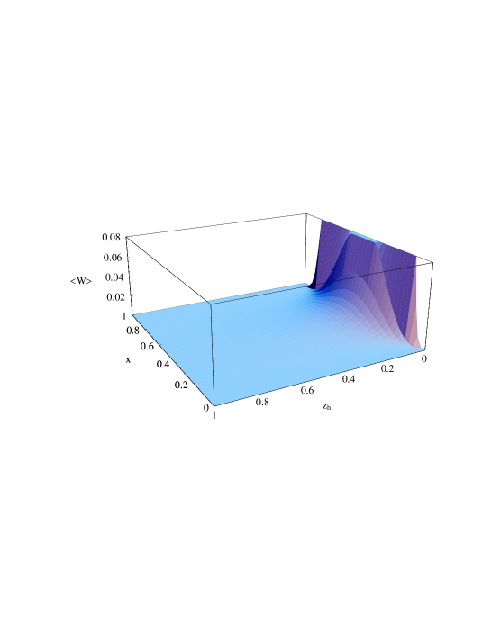
Figure 5: A tri-dimensional view of the quantity $\sum_{a,\overline{a}}e_{a}^{2}\ x\,f_{1T}^{\perp(1)a}(x)\,D_{1}^{a}(z_{h})$, directly proportional to the T-odd distribution function $f_{1T}^{\perp}(x)$, for production of $\pi^{+}$ on a transversely polarized proton. Only valence contributions are taken into account. Here the function becomes sizeable for small values of $z_{h}$ but intermediate values of $x$.

 

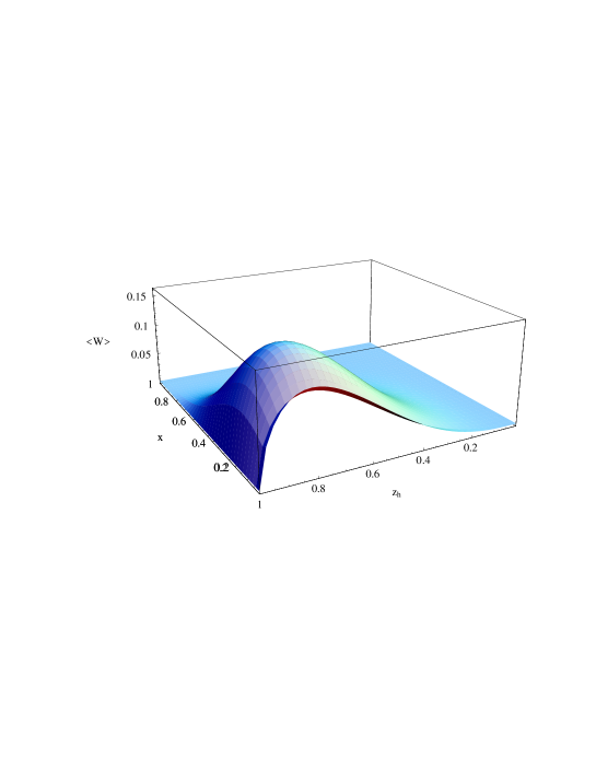
Figure 6: A tri-dimensional view of $\sum_{a,\overline{a}}e_{a}^{2}x\,h_{1}^{a}(x)\,H_{1}^{\perp(1)a}(z_{h})$, directly proportional to the T-odd fragmentation function $H_{1}^{\perp}(z_{h})$ production of $\pi^{+}$ on a transversely polarized proton. Once again, only valence contributions are taken into account. As opposed to the above case, here the function reaches its maximum for considerably larger values of $z_{h}$.

5 Concluding remarks

In the previous section some results for 1-particle inclusive lepton-hadron scattering have been presented. Several other effects are important in these cross sections, such as target fragmentation, the inclusion of gluons in the calculation to obtain color-gauge invariant definitions of the correlation functions and an electromagnetically gauge invariant result at order $1/Q$ and finally QCD corrections which can be moved back and forth between hard and soft parts, leading to the scale dependence of the soft parts and the DGLAP equations$\!{}^{{\bf?}}$.

In my talk I have tried to indicate why semi-inclusive, in particular 1-particle inclusive lepton-hadron scattering, can be important. The goal is the study of the quark and gluon structure of hadrons, emphasizing the dependence on transverse momenta of quarks. The reason why this prospect is promising is the existence of a field theoretical framework that allows a clean study involving well-defined hadronic matrix elements. EPIC is needed to provide the experimental requirements for a detailed study, such as polarized targets and detection of final state hadrons and their polarization via study of decay configurations over a sufficiently large range of energies and momentum transfer.

References

References

• [1] D.E. Soper, Phys. Rev. D 15 (1977) 1141; Phys. Rev. Lett. 43 (1979) 1847.
• [2] R.L. Jaffe, Nucl. Phys. B 229 (1983) 205.
• [3] J.C. Collins and D.E. Soper, Nucl. Phys. B 194 (1982) 445.
• [4] R.L. Jaffe and X. Ji, Nucl. Phys. B 375 (1992) 527.
• [5] N. Hammon, O. Teryaev and A. Schäfer, Phys. Lett. B390 (1997) 409; D. Boer, P.J. Mulders and O.V. Teryaev, Phys. Rev. D57 (1998) 3057.
• [6] D. Sivers, Phys. Rev. D41 (1990) 83 and Phys. Rev. D43 (1991) 261 and
• [7] M. Anselmino, M. Boglione and F. Murgia, Phys. Lett. B362 (1995) 164; M. Anselmino and F. Murgia, Phys. Lett. B442 (1998) 470.
• [8] A.P. Bukhvostov, E.A. Kuraev and L.N. Lipatov, Sov. Phys. JETP 60 (1984) 22.
• [9] R.D. Tangerman and P.J. Mulders, Nucl. Phys. B461 (1996) 197.
• [10] M. Anselmino, A. Drago and F. Murgia, hep-ph/9703303.
• [11] J. Levelt and P.J. Mulders, Phys. Rev. D 49 (1994) 96; Phys. Lett. B 338 (1994) 357.
• [12] J. Collins, Nucl. Phys. B396 (1993) 161.
• [13] M. Anselmino, M. Boglione and F. Murgia, hep-ph/9901442.
• [14] M. Boglione and P.J. Mulders, Time-reversal odd fragmentation and distribution functions in pp and ep single spin asymmetries, hep-ph/9903354, to be publ. in Phys. Rev. D
• [15] P.J. Mulders, in Proceedings of the 2. ELFE Workshop, St. Malo, 23-27 Sept. 1996, nucl-th/9611040.