Determining SUSY Parameters from Chargino Pair Production

Abstract:

A procedure to determine the chargino mixing angles and, subsequently, the fundamental SUSY parameters $M_{2},\mu$ and $\tan\beta$ by measurements of the total cross section and the spin correlations in $e^{+}e^{-}$ annihilation to $\tilde{\chi}_{1}^{+}\tilde{\chi}_{1}^{-}$ chargino pairs is discussed.

1 Introduction

Despite the lack of direct experimental evidence for supersymmetry (SUSY), the concept of symmetry between bosons and fermions [1] has so many attractive features that the supersymmetric extension of the Standard Model is widely considered as a most natural scenario. SUSY ensures the cancellation of quadratically divergent corrections from scalar and fermion loops and thus stabilizes the Higgs boson mass in the desired range of order $10^{2}$ GeV, predicts the renormalized electroweak mixing angle $\sin^{2}\theta_{W}$ in striking agreement with the measured value, and provides the opportunity to generate the electroweak symmetry breaking radiatively.

Supersymmetry predicts the quarks and leptons to have scalar partners, called squarks and sleptons, the gauge bosons to have fermionic partners, called gauginos. In the Minimal Supersymmetric Standard Model (MSSM) [2] two Higgs doublets with opposite hypercharges, and with their superpartners: higgsinos, are required to give masses to the up and down type fermions and to ensure anomaly cancellation. The higgsinos and electroweak gauginos mix; the mass eigenstates are called charginos $\tilde{\chi}_{1,2}^{\pm}$ and neutralinos $\tilde{\chi}_{1,2,3,4}^{0}$ for electrically charged and neutral states, respectively. Actually in many supersymmetric models the lighter chargino states $\tilde{\chi}_{1}^{\pm}$ are expected to be the lightest observable supersymmetric particles and they may play an important role in the first direct experimental evidence for supersymmetry.

The doubling of the spectrum of states in the MSSM together with our ignorance on the dynamics of the supersymmetry breaking mechanisms gives rise to a large number of unknown parameters. Even with the $R$-parity conserving and CP-invariant SUSY sector, which we will assume in what follows, in total more than 100 new parameters are introduced. This number of parameters can be reduced by additional physical assumptions. In the literature several theoretically motivated scenarios have been considered. The most radical reduction is achieved by embedding the low–energy supersymmetric theory into a grand unified (SUSY-GUT) framework called mSUGRA. The mSUGRA is fully specified at the GUT scale by a common gaugino mass $m_{1/2}$, a common scalar mass $m_{0}$, a common trilinear scalar coupling $A_{G}$, the ratio $\tan\beta=v_{2}/v_{1}$ of the vev’s of the two neutral Higgs fields, and the sign of the Higgs mass parameter $\mu$. All the couplings, masses and mixings at the electroweak scale are then determined by the RGEs [3]. It turns out, however, that the interpretation of experimental data and derived limits on sparticle masses and their couplings strongly depends on the adopted scenario. Therefore it is important to develop strategies to measure all low-energy SUSY parameters independently of any theoretical assumptions. The experimental program to search for and explore SUSY at present and future colliders should thus include the following points:

• discover supersymmetric particles and measure their quantum numbers to prove that they are superpartners of standard particles,

• determine the low-energy Lagrangian parameters,

• verify the relations among them in order to distinguish between various SUSY models.

If SUSY is realized in Nature, it will be a matter of days for the future $e^{+}e^{-}$ linear colliders (LC) to discover the kinematically accessible supersymmetric particles. Once they are discovered, the priority will be to measure the low-energy SUSY parameters independently of theoretical prejudices and then check whether the correlations among parameters, if any, support a given theoretical framework [4], like SUSY-GUT relations. Particularly in this respect the $e^{+}e^{-}$ linear colliders are indispensable tools, as has been demonstrated in a number of dedicated workshops [5]. In my talk I will concentrate on the first phase of LC, $i.e.$ when only a limited number of supersymmetric particles can kinematically be produced. In contrast to earlier analyses [6, 7], I will not elaborate on global chargino/neutralino fits but rather attempt to explore the event characteristics to isolate the chargino sector. The analysis will be based strictly on low–energy supersymmetry. We will see that even if the lightest chargino states $\tilde{\chi}_{1}^{\pm}$ are, before the collider energy upgrade, the only supersymmetric states that can be explored experimentally in detail, some of the fundamental SUSY parameters can be reconstructed from the measurement of chargino mass $m_{\tilde{\chi}_{1}^{\pm}}$, the total production cross section and the chargino polarization in the final state. Beam polarization is helpful but not necessarily required.

The results presented here have been obtained in collaboration with S.Y. Choi, A. Djouadi, H. Dreiner and P. Zerwas [8]. For an alternative way of determining the SUSY parameters from the measurement of (some) chargino and neutralino masses, see [9].

2 Chargino masses and couplings

The superpartners of the $W$ boson and charged Higgs boson, $\tilde{W}^{\pm}$ and $\tilde{H}^{\pm}$, necessarily mix since the mass matrix (in the $\{\tilde{W}^{-},\tilde{H}^{-}\}$ basis) [2]

$${\cal M}_{C}=\left(\begin{array}[]{cc}M_{2}&\sqrt{2}m_{W}c_{\beta}\\ \sqrt{2}m_{W}s_{\beta}&\mu\end{array}\right)$$ (3)

is nondiagonal ($c_{\beta}=\cos\beta$, $s_{\beta}=\sin\beta$). It is expressed in terms of the fundamental supersymmetric parameters: the gaugino mass $M_{2}$, the Higgs mass parameter $\mu$, and $\tan\beta$. Two different matrices acting on the left– and right–chiral $(\tilde{W},\tilde{H})$ states are needed to diagonalize the asymmetric mass matrix (3). The (positive) eigenvalues are given by

$$m^{2}_{\tilde{\chi}^{\pm}_{1,2}}={\textstyle\frac{1}{2}}\left[M^{2}_{2}+\mu^{2}+2m^{2}_{W}\mp\Delta\,\right]$$ (4)

where

$$\Delta= [(M^{2}_{2}+\mu^{2}+2m^{2}_{W})^{2}$$ (5)

$$-4(M_{2}\mu-m^{2}_{W}\sin 2\beta)^{2}]^{1/2}$$

The left– and right–chiral components of the corresponding chargino mass eigenstate $\tilde{\chi}^{-}_{1}$ are related to the wino and higgsino components in the following way

$$\tilde{\chi}^{-}_{1L}=\tilde{W}^{-}_{L}\cos\phi_{L}+\tilde{H}^{-}_{1L}\sin\phi_{L}$$

$$\tilde{\chi}^{-}_{1R}=\tilde{W}^{-}_{R}\cos\phi_{R}+\tilde{H}^{-}_{2R}\sin\phi_{R}$$ (6)

with the rotation angles given by

$$\cos 2\phi_{L}=-(M_{2}^{2}-\mu^{2}-2m^{2}_{W}\cos 2\beta)/\Delta~{}~{}~{}~{}~{}~{}~{}~{}$$

$$\cos 2\phi_{R}=-(M_{2}^{2}-\mu^{2}+2m^{2}_{W}\cos 2\beta)/\Delta$$ (7)

As usual, we take $\tan\beta$ positive, $M_{2}$ positive and $\mu$ of either sign.

The angles $\phi_{L}$ and $\phi_{R}$ determine the $\tilde{\chi}\tilde{\chi}Z$ and the $\tilde{\chi}\tilde{\nu}e$ couplings:

$$\langle\tilde{\chi}^{-}_{1L}|Z|\tilde{\chi}^{-}_{1L}\rangle=-\frac{e}{4s_{W}c_{W}}(4s_{W}^{2}-3-\cos 2\phi_{L})$$

$$\langle\tilde{\chi}^{-}_{1R}|Z|\tilde{\chi}^{-}_{1R}\rangle=-\frac{e}{4s_{W}c_{W}}(4s_{W}^{2}-3-\cos 2\phi_{R})$$

$$\langle\tilde{\chi}^{-}_{1R}|\tilde{\nu}|e^{-}_{L}\rangle=-\frac{e}{s_{W}}\cos\phi_{R}$$ (8)

where $s_{W}^{2}=1-c_{W}^{2}\equiv\sin^{2}\theta_{W}$. The coupling to the higgsino component, being proportional to the electron mass, has been neglected in the sneutrino vertex. The photon–chargino vertex is diagonal, $i.e.$ it is independent of the mixing angles:

$$\langle\tilde{\chi}^{-}_{1L,R}|\gamma|\tilde{\chi}^{-}_{1L,R}\rangle=e$$ (9)

The chargino couplings, and therefore mixing angles, are physical observables and they can be measured. Their knowledge together with the measurement of the chargino masses is sufficient to determine the fundamental supersymmetric parameters $M_{2}$, $\mu$ and $\tan\beta$.

3 Chargino production and decay

Charginos are produced in $e^{+}e^{-}$ collisions, either in diagonal or in mixed pairs. Here we will consider the diagonal pair production of the lightest chargino $\tilde{\chi}_{1}^{\pm}$ in $e^{+}e^{-}$ collisions,

$$e^{+}e^{-}\ \rightarrow\ \tilde{\chi}^{+}_{1}\ \tilde{\chi}^{-}_{1}$$ (10)

assuming the second chargino $\tilde{\chi}_{2}^{\pm}$ too heavy to be produced in the first phase of $e^{+}e^{-}$ linear colliders. If the chargino production angle could be measured unambiguously on an event-by-event basis, the chargino couplings could be extracted directly from the angular dependence of the cross section. However, charginos are not stable. We will assume that they decay into the lightest neutralino $\tilde{\chi}^{0}_{1}$, which is taken to be stable, and a pair of quarks and antiquarks or charged leptons and neutrinos. Since two neutral particles $\tilde{\chi}^{0}_{1}$ escape undetected, it is not possible to reconstruct the events unambiguously. In particular the production angle $\Theta$ cannot be reconstructed for a given event. The distribution of observed final state quark jets or leptons is given by a convolution of the chargino production and decay processes. Therefore we will consider the production of polarized charginos and their subsequent decays. It has to be stressed that the spin correlations between production and decay have to be properly taken into account [7, 8].

3.1 Polarized chargino production

The process $e^{+}e^{-}\rightarrow\tilde{\chi}^{+}_{1}\tilde{\chi}^{-}_{1}$ is generated by the three mechanisms shown in Fig. 1: $s$–channel $\gamma$ and $Z$

Figure 1: The three mechanisms contributing to the production of diagonal chargino pairs $\tilde{\chi}^{+}_{1}\tilde{\chi}^{-}_{1}$ in $e^{+}e^{-}$ annihilation.

exchanges, and $t$–channel $\tilde{\nu}$ exchange. After a Fierz transformation of the $\tilde{\nu}$–exchange term, the amplitude

$$T= \frac{e^{2}}{s}Q_{\alpha\beta}[\bar{v}(e^{+})\gamma_{\mu}P_{\alpha}u(e^{-})]$$ (11)

$$\times[\bar{u}(\tilde{\chi}^{-}_{1})\gamma^{\mu}P_{\beta}v(\tilde{\chi}^{+}_{1})]$$

can be expressed in terms of four bilinear charges, classified according to the chiralities of the associated lepton ($\alpha=L,R$) and chargino ($\beta=L,R$) currents

$$Q_{L\beta}= 1+\frac{D_{Z}}{8s_{W}^{2}c_{W}^{2}}(2s_{W}^{2}-1)(4s_{W}^{2}-3-\cos 2\phi_{\beta})$$

$${}+\delta_{\beta,R}\frac{D_{\tilde{\nu}}}{4s_{W}^{2}}(1+\cos 2\phi_{R})$$

$$Q_{R\beta}= 1+\frac{D_{Z}}{4c_{W}^{2}}(4s_{W}^{2}-3-\cos 2\phi_{\beta})$$ (12)

The $\tilde{\nu}$ exchange affects only the $LR$ charge while all other charges are built up by $\gamma$ and $Z$ exchanges. $D_{\tilde{\nu}}$ denotes the sneutrino propagator $D_{\tilde{\nu}}=s/(t-m_{\tilde{\nu}}^{2})$, and $D_{Z}$ the $Z$ propagator $D_{Z}=s/(s-m^{2}_{Z}+im_{Z}\Gamma_{Z})$. Above the $Z$ pole the non–zero width can be neglected so that the charges are real.

The $\tilde{\chi}^{-}_{1}$ and $\tilde{\chi}^{+}_{1}$ helicities are in general not correlated due to the non–zero masses of the particles; amplitudes with equal $\tilde{\chi}^{\pm}_{1}$ helicities vanish only $\propto m_{\tilde{\chi}^{\pm}_{1}}/\sqrt{s}$ for asymptotic energies. Denoting the electron helicity by the first index $\sigma$ and the $\tilde{\chi}^{-}_{1}$ and $\tilde{\chi}^{+}_{1}$ helicities by the remaining two indices $\lambda$ and $\bar{\lambda}$, the helicity amplitudes $T(\sigma;\lambda\bar{\lambda})=2\pi\alpha{\cal A}_{\sigma;\lambda\bar{\lambda}}$ can be expressed as functions of bilinear chirality charges [10]

$${\cal A}_{+;++}=-\sqrt{\beta_{-}\beta_{+}}(Q_{RR}+Q_{RL})\sin\Theta$$

$${\cal A}_{+;+-}=-(\beta_{+}Q_{RR}+\beta_{-}Q_{RL})(1+\cos\Theta)$$

$${\cal A}_{+;-+}=+(\beta_{-}Q_{RR}+\beta_{+}Q_{RL})(1-\cos\Theta)$$

$${\cal A}_{+;--}=+\sqrt{\beta_{-}\beta_{+}}(Q_{RR}+Q_{RL})\sin\Theta$$

$${\cal A}_{-;++}=-\sqrt{\beta_{-}\beta_{+}}(Q_{LR}+Q_{LL})\sin\Theta$$

$${\cal A}_{-;+-}=+(\beta_{+}Q_{LR}+\beta_{-}Q_{LL})(1-\cos\Theta)$$

$${\cal A}_{-;-+}=-(\beta_{-}Q_{LR}+\beta_{+}Q_{LL})(1+\cos\Theta)$$

$${\cal A}_{-;--}=+\sqrt{\beta_{-}\beta_{+}}(Q_{LR}+Q_{LL})\sin\Theta$$ (13)

where $\beta_{\pm}=1\pm\beta$, and $\beta=(1-4m^{2}_{\tilde{\chi}^{\pm}_{1}}/s)^{1/2}$ is the $\tilde{\chi}^{\pm}_{1}$ velocity in the c.m. frame.

The unpolarized differential cross section for $e^{+}e^{-}\rightarrow\tilde{\chi}^{+}_{1}\tilde{\chi}^{-}_{1}$ is obtained by averaging/summing over the electron/chargino helicities. It can be written as

$$\frac{{\rm d}\sigma}{{\rm d}\cos\Theta} =\frac{\pi\alpha^{2}}{2s}\beta\{(1+\beta^{2}\cos^{2}\Theta)Q_{1}$$ (14)

$$+(1-\beta^{2})Q_{2}+2\beta\cos\Theta Q_{3}\}~{}~{}~{}~{}~{}$$

where the quartic charges $Q_{i}$ are given in terms of bilinear charges as follows [11]

$$Q_{1}={\textstyle\frac{1}{4}}(|Q_{RR}|^{2}+|Q_{LL}|^{2}+|Q_{RL}|^{2}+|Q_{LR}|^{2})$$

$$Q_{2}={\textstyle\frac{1}{2}}{\rm Re}(Q_{RR}Q^{*}_{RL}+Q_{LL}Q^{*}_{LR})$$ (15)

$$Q_{3}={\textstyle\frac{1}{4}}(|Q_{RR}|^{2}+|Q_{LL}|^{2}-|Q_{RL}|^{2}-|Q_{LR}|^{2})$$

Figure 2: Left panel: the total cross section as a function of the c.m.energy. Right panel: the angular distribution as a function of the production angle for $\sqrt{s}=500$ GeV. In both panels: $m_{\tilde{\nu}}=200$ GeV, solid lines for the gaugino, dashed lines for the higgsino and dot-dashed lines for the mixed cases, see eq. 19 [taken from [8]].

The total production cross section as a function of the c.m.energy and the angular distribution at $\sqrt{s}=500$ GeV are shown in Fig. 2 for a representative set of ($M_{2},\mu$) parameters; the sneutrino mass has been taken $m_{\tilde{\nu}}=200$ GeV. The parameters are chosen in the higgsino region $M_{2}\gg|\mu|$, the gaugino region $M_{2}\ll|\mu|$ and in the mixed region $M_{2}\sim|\mu|$ for $\tan\beta=2$ as (in GeV)

$$\begin{array}[]{ll}{\rm gaugino}:&(M_{2},\mu)=(81,\,-215)\\ {\rm higgsino}:&(M_{2},\mu)=(215,\,-81)\\ {\rm mixed}:&(M_{2},\mu)=(92,\,-93)\end{array}$$ (19)

for which the light chargino mass $m_{\tilde{\chi}^{\pm}_{1}}$ is approximately $95$ GeV. The sharp rise of the production cross section in Fig. 2 allows us to measure the chargino mass $m_{\tilde{\chi}^{\pm}_{1}}$ very precisely. As is well-known, the sneutrino exchange leads to a strong destructive interference for the gaugino and mixed regions, while the dependence of the cross section on $m_{\tilde{\nu}}$ decreases as the higgsino component of the chargino increases. Prior or simultaneous determination of $m_{\tilde{\nu}}$ is therefore necessary to determine the other SUSY parameters.

In general charginos are produced with non-zero polarization. The key point in our analysis in Sect. 4 will be to exploit the partial information on the chargino polarizations that can be obtained from the distribution of the chargino decay products. Therefore we define the $\tilde{\chi}^{-}_{1}$ polarization vector $\vec{\cal P}=({\cal P}_{T},{\cal P}_{N},{\cal P}_{L})$ in the $\tilde{\chi}^{-}_{1}$ rest frame. ${\cal P}_{L}$ denotes the component parallel to the $\tilde{\chi}^{-}_{1}$ flight direction in the c.m. frame, ${\cal P}_{T}$ the transverse component in the production plane, and ${\cal P}_{N}$ the component normal to the production plane. The three components can be written in terms the helicity amplitudes as

$${\cal P}_{L}={\frac{1}{4{\cal N}}}\sum_{\sigma=\pm}(|{\cal A}_{\sigma;++}|^{2}+|{\cal A}_{\sigma;+-}|^{2}\rule{56.9055pt}{0.0pt}$$

$$-|{\cal A}_{\sigma;-+}|^{2}-|{\cal A}_{\sigma;--}|^{2})\rule{56.9055pt}{0.0pt}$$ (20)

$${\cal P}_{T}=\frac{1}{2{\cal N}}\sum_{\sigma=\pm}{\rm Re}({\cal A}_{\sigma;++}{\cal A}_{\sigma;-+}^{*}+{\cal A}_{\sigma;--}{\cal A}_{\sigma;+-}^{*})$$

$${\cal P}_{N}={\frac{1}{2{\cal N}}}\sum_{\sigma=\pm}{\rm Im}({\cal A}_{\sigma;--}{\cal A}_{\sigma;+-}^{*}-{\cal A}_{\sigma;++}{\cal A}_{\sigma;-+}^{*})$$

with the normalization

$${\cal N}={\frac{1}{4}}\sum_{\sigma=\pm}(|{\cal A}_{\sigma;++}|^{2}+|{\cal A}_{\sigma;+-}|^{2}\rule{56.9055pt}{0.0pt}$$

$$+|{\cal A}_{\sigma;-+}|^{2}+|{\cal A}_{\sigma;--}|^{2})\rule{42.67912pt}{0.0pt}$$ (21)

The normal component ${\cal P}_{N}$ can only be generated by complex production amplitudes. Neglecting small higher order loop effects and the small $Z$–width effect, the normal $\tilde{\chi}^{-}_{1}$ and $\tilde{\chi}^{+}_{1}$ polarizations are zero since the $\tilde{\chi}_{1}\tilde{\chi}_{1}\gamma$ and $\tilde{\chi}_{1}\tilde{\chi}_{1}Z$ vertices are real (even for non-zero phases in the chargino mass matrix) and the $\tilde{\nu}$–exchange amplitude is real too. The CP–violating phases will change the chargino mass and the mixing angles [8, 13] but they do not induce complex charges in the production amplitudes of the diagonal chargino pairs.

3.2 Decay of polarized charginos

We will assume that charginos decay into the lightest neutralino $\tilde{\chi}^{0}_{1}$ and a pair of quarks and antiquarks or leptons and neutrinos: $\tilde{\chi}^{\pm}_{1}\rightarrow\tilde{\chi}^{0}_{1}+f\bar{f}^{\prime}$. The decay can proceed via the exchange of the $W$, squarks or sleptons; the exchange of the charged Higgs bosons can be neglected for light fermions in the final state. The corresponding diagrams are shown in Fig. 3 for the decay into quark pairs.

Figure 3: Chargino decay mechanisms; the exchange of the charged Higgs boson is neglected.

After a Fierz transformation of the $\tilde{q}$–exchange contributions, the decay amplitude $\tilde{\chi}^{-}_{1}\rightarrow\tilde{\chi}^{0}_{1}d\bar{u}$ may be written as:

$${\cal D}= \frac{e^{2}}{2\sqrt{2}s_{W}^{2}}[\bar{u}(d)\gamma^{\mu}P_{L}v(\bar{u})]$$ (22)

$$\times[\bar{u}(\tilde{\chi}^{0}_{1})\gamma_{\mu}(F_{L}P_{L}+F_{R}P_{R})u(\tilde{\chi}^{-}_{1})]~{}~{}~{}$$

with

$$F_{L} =D_{W}(2N_{12}\cos\phi_{L}+\sqrt{2}N_{13}\sin\phi_{L})$$

$${}+D_{\tilde{d}_{L}}\cos\phi_{L}(N_{12}-2Y_{q}\tan\theta_{W}N_{11})$$

$$F_{R} =D_{W}(2N^{*}_{12}\cos\phi_{R}-\sqrt{2}N^{*}_{14}\sin\phi_{R})$$ (23)

$${}+D_{\tilde{u}_{L}}\cos\phi_{R}(N^{*}_{12}+2Y_{q}\tan\theta_{W}N^{*}_{11})~{}~{}~{}~{}~{}$$

where $Y_{q}=1/6$ is the quark hypercharge and $D_{W}=s^{\prime}-m^{2}_{W}+im_{W}\Gamma_{W}$, $D_{\tilde{d}_{L}}=t^{\prime}-m^{2}_{\tilde{d}_{L}}$, $D_{\tilde{u}_{L}}=u^{\prime}-m^{2}_{\tilde{u}_{L}}$. Analogous expressions apply to decays into lepton pairs with $Y_{l}=-1/2$. The Mandelstam variables $s^{\prime}$, $t^{\prime}$, $u^{\prime}$ are defined in terms of the 4–momenta $q_{0},q$ and $\bar{q}$ of $\tilde{\chi}_{1}^{0},d$ and $\bar{u}$, respectively, as $s^{\prime}=(q+\bar{q})^{2}$, $t^{\prime}=(q_{0}+q)^{2}$, $u^{\prime}=(q_{0}+\bar{q})^{2}$, while $N_{ij}$ is the $4\times 4$ matrix rotating the current neutralino eigenstates $\tilde{B},\tilde{W}^{3},\tilde{H}^{0}_{1},\tilde{H}^{0}_{2}$ to the mass eigenstates $\tilde{\chi}^{0}_{1},..,\tilde{\chi}^{0}_{4}$. The neutralino mass matrix ${\cal M}_{N}$ is given by

$$\left[\begin{array}[]{cccc}M_{1}&0&-m_{Z}s_{W}c_{\beta}&m_{Z}s_{W}s_{\beta}\\ 0&M_{2}&m_{Z}c_{W}c_{\beta}&-m_{Z}c_{W}s_{\beta}\\ -m_{Z}s_{W}c_{\beta}&m_{Z}c_{W}c_{\beta}&0&-\mu\\ m_{Z}s_{W}s_{\beta}&-m_{Z}c_{W}s_{\beta}&-\mu&0\end{array}\right]$$ (28)

Besides the parameters $M_{2},\mu$ and $\tan\beta$, which already appear in the chargino mass matrix, the only additional parameter in the neutralino mass matrix is $M_{1}$. In general supersymmetric models, however, the neutralino sector can potentially be more complex than in the MSSM with more additional parameters.

In the chargino rest frame, the angular distribution of the neutralino and the $f_{1}\bar{f}_{2}$ system from the polarized chargino decay $\tilde{\chi}^{\pm}_{1}\rightarrow\tilde{\chi}^{0}_{1}+f_{1}\bar{f}_{2}$ (summed over the final state polarizations) is determined by the energy and the polar angle of the neutralino (or equivalently of the $f_{1}\bar{f}_{2}$ system) with respect to the chargino polarization vector. Let us define $\theta^{*}$ ($\bar{\theta}^{*}$) as the polar angle of the $f_{1}\bar{f}_{2}$ ($\bar{f}_{3}f_{4}$) system in the $\tilde{\chi}^{-}_{1}$ ($\tilde{\chi}^{+}_{1}$) rest frame with respect to the original flight direction in the laboratory frame, and $\phi^{*}$($\bar{\phi}^{*}$) the corresponding azimuthal angle with respect to the production plane. Taking the $\tilde{\chi}^{-}_{1}$ ($\tilde{\chi}^{+}_{1}$) flight direction as quantization axis and for the kinematical configuration defined above, the spin–density matrix $\rho_{\lambda\lambda^{\prime}}\sim{\cal D}_{\lambda}{\cal D}^{*}_{\lambda^{\prime}}$ can conveniently be written in the following form

$$\rho_{\lambda\lambda^{\prime}}=\frac{1}{2}\left(\begin{array}[]{cc}1+\kappa\cos\theta^{*}&\kappa\sin\theta^{*}{\rm e}^{i\phi^{*}}\\ \kappa\sin\theta^{*}{\rm e}^{-i\phi^{*}}&1-\kappa\cos\theta^{*}\end{array}\right)~{}~{}~{}$$ (31)

for the $\tilde{\chi}^{-}_{1}$ decay, and similarly for the $\tilde{\chi}^{+}_{1}$ with barred quantities.

Figure 4: The polarization analysis–power $\kappa$ as a function of the hadron invariant mass $\sqrt{s^{\prime}}$ for the same set of parameters as for the cross section (19).

The spin analysis–powers $\kappa$ and $\bar{\kappa}$, depend on the final $ud$ or $l\nu$ pairs considered in the chargino decays. Since left– and right–chiral form factors $F_{L},F_{R}$ contribute at the same time, their values are determined by the masses and couplings of all the particles involved in the decay. Characteristic examples for $\kappa$ as a function of the invariant mass of the fermion system are shown in Fig. 4; the squark masses are set to 300 GeV, and the gaugino masses are assumed universal at the unification scale. For our purposes, however, it will suffice that they are finite. Let us also note that neglecting effects from non–zero widths, loops and CP–noninvariant phases, $\kappa$ and $\bar{\kappa}$ are real, and $\kappa=-\bar{\kappa}$ for charginos $\tilde{\chi}^{\pm}_{1}$ decaying to charge-conjugated final states.

3.3 Physical observables

Charginos decay fast and only correlated production and decay can be observed experimentally. The matrix element for the physical process

$$e^{+}e^{-}\rightarrow\tilde{\chi}^{-}_{1}\tilde{\chi}^{+}_{1}\rightarrow(\tilde{\chi}^{0}_{1}f_{1}\bar{f}_{2})(\tilde{\chi}^{0}_{1}\bar{f}_{3}f_{4})~{}~{}~{}~{}~{}$$ (32)

summed/averaged over the final/initial state polarizations, is given by ${\cal M}=\sum T_{\sigma;\lambda\bar{\lambda}}{\cal D}_{\lambda}\overline{\cal D}_{\bar{\lambda}}$. Integrating over the production angle $\Theta$ and also over the invariant masses of the fermionic systems $(f_{1}\bar{f}_{2})$ and $(\bar{f}_{3}f_{4})$, one can write the 4-fold differential cross section in the following form:

$$\frac{d^{4}\sigma}{d\cos\theta^{*}d\phi^{*}d\cos\bar{\theta}^{*}d\bar{\phi}^{*}}=\frac{\alpha^{2}\beta}{124\pi s}{\cal B}\,\bar{\cal B}\,\Sigma~{}~{}~{}~{}$$ (33)

where ${\cal B}=Br(\tilde{\chi}_{1}^{-}\to\tilde{\chi}_{1}^{0}f_{1}\bar{f}_{2})$ and ${\bar{\cal B}}=Br(\tilde{\chi}_{1}^{+}\to\tilde{\chi}_{1}^{0}\bar{f}_{3}f_{4})$. The scaled differential cross section $\Sigma=\Sigma(\theta^{*},\phi^{*},\bar{\theta}^{*},\bar{\phi}^{*})$ is a product of the production helicity amplitudes ${\cal A}_{\sigma;\lambda\bar{\lambda}}$ and the spin density matrices for the chargino decays $\rho_{\lambda\lambda^{\prime}}$

$$\Sigma=\sum_{\lambda\bar{\lambda}}\sum_{\lambda^{\prime}\bar{\lambda}^{\prime}}\sum_{\sigma}{\cal A}_{\sigma;\lambda\bar{\lambda}}{\cal A}^{*}_{\sigma;\lambda^{\prime}\bar{\lambda}^{\prime}}\,\rho_{\lambda\lambda^{\prime}}\bar{\rho}_{\bar{\lambda}\bar{\lambda}^{\prime}}$$ (34)

The quantity $\Sigma$ can be decomposed into sixteen independent angular parts

$$\Sigma = \Sigma_{\rm un}+\cos\theta^{*}\kappa{\cal P}+\cos\bar{\theta}^{*}\bar{\kappa}\bar{\cal P}$$ (35)

$$+\cos\theta^{*}\cos\bar{\theta}^{*}\kappa\bar{\kappa}{\cal Q}$$

$$+\sin\theta^{*}\sin\bar{\theta}^{*}\cos(\phi^{*}+\bar{\phi}^{*})\kappa\bar{\kappa}{\cal Y}$$

$$+\sin\theta^{*}\sin\bar{\theta}^{*}\sin(\phi^{*}+\bar{\phi}^{*})\kappa\bar{\kappa}\bar{\cal Y}$$

$$+\sin\theta^{*}\cos\phi^{*}\kappa{\cal U}+\sin\theta^{*}\sin\phi^{*}\kappa\bar{\cal U}$$

$$+\sin\bar{\theta}^{*}\cos\bar{\phi}^{*}\bar{\kappa}{\cal V}+\sin\bar{\theta}^{*}\sin\bar{\phi}^{*}\bar{\kappa}\bar{\cal V}$$

$$+\sin\theta^{*}\cos\bar{\theta}^{*}(\cos\phi^{*}\kappa\bar{\kappa}{\cal W}+\sin\phi^{*}\kappa\bar{\kappa}\bar{\cal W})$$

$$+\cos\theta^{*}\sin\bar{\theta}^{*}(\cos\bar{\phi}^{*}\kappa\bar{\kappa}{\cal X}+\sin\bar{\phi}^{*}\kappa\bar{\kappa}\bar{\cal X})$$

$$+\sin\theta^{*}\sin\bar{\theta}^{*}(\cos(\phi^{*}-\bar{\phi}^{*})\kappa\bar{\kappa}{\cal Z}$$

$$+\sin\theta^{*}\sin\bar{\theta}^{*}(\sin(\phi^{*}-\bar{\phi}^{*})\kappa\bar{\kappa}\bar{\cal Z}$$

where the sixteen coefficients are combinations of helicity amplitudes, corresponding to the unpolarized cross section ($\Sigma_{\rm un}$), $2\times 3$ polarization components (${\cal P,U,V},\bar{\cal P},\bar{\cal U},\bar{\cal V}$) and $3\times 3$ spin–spin correlations (the remaining ones) multiplied by the spin-analysis power factors $\kappa$ and $\bar{\kappa}$. In the CP-invariant theory, and neglecting loops and the width of the $Z$–boson for high energies, the six functions $\bar{\cal U},\bar{\cal V},\bar{\cal W},\bar{\cal X},\bar{\cal Y},\bar{\cal Z}$ can be discarded. Moreover, from CP–invariance

$${\cal A}_{\sigma;\lambda\lambda^{\prime}}=(-1)^{\lambda-\lambda^{\prime}-1}{\cal A}_{\sigma;-\lambda^{\prime}-\lambda}$$ (36)

it follows that $\bar{\cal P}=-{\cal P}$, ${\cal U}=-{\cal V}$ and ${\cal W}={\cal X}$. The overall topology is therefore determined by seven independent functions: $\Sigma_{\rm un}$, ${\cal P}$, ${\cal Q}$, ${\cal U}$, ${\cal W}$, ${\cal Y}$ and ${\cal Z}$.

The key point in our analysis is to exploit the partial information on the chargino polarizations with which they are produced. The $\tilde{\chi}$ polarization vectors and $\tilde{\chi}$–$\tilde{\chi}$ spin–spin correlation tensors can be determined from the decay distributions of the charginos independently of the chargino decay dynamics.

The decay angles $(\theta^{*},\phi^{*})$ and $(\bar{\theta}^{*},\bar{\phi}^{*})$, which are used to measure the $\chi_{1}^{\pm}$ chiralities, can not be reconstructed completely since there are two invisible neutralinos in the final state. However, the longitudinal components and the inner product of the transverse components can be reconstructed from the momenta measured in the laboratory frame

$$\cos\theta^{*}=({E}-{\gamma}E^{*})/{\beta{\gamma}|\vec{p}^{*}|}$$

$$\cos\bar{\theta}^{*}=({\bar{E}}-{\gamma}\bar{E}^{*})/{\beta{\gamma}|\vec{\bar{p}}^{*}|}$$

$$\sin\theta^{*}\sin\bar{\theta}^{*}\cos(\phi^{*}+\bar{\phi}^{*})={\vec{p}\cdot\vec{\bar{p}}}/{|\vec{p}^{*}||\vec{\bar{p}}^{*}|}~{}~{}~{}~{}$$

$$+(\gamma E-E^{*})(\gamma\bar{E}-\bar{E}^{*})/{\beta^{2}\gamma^{2}|\vec{p}^{*}||\vec{\bar{p}}^{*}|}$$ (37)

where $\gamma=\sqrt{s}/{2m_{\tilde{\chi}^{\pm}_{1}}}$. $E(\bar{E})$ and $E^{*}(\bar{E}^{*})$ are the energies of the two hadronic systems in the laboratory frame and in the rest frame of the charginos, respectively; $\vec{p}(\vec{\bar{p}})$ and $\vec{p}^{*}(\vec{\bar{p}^{*}})$ are the corresponding momenta; the angle between the vectors in the transverse plane is given by $\Delta\phi^{*}=2\pi-(\phi^{*}+\bar{\phi}^{*})$ for the reference frames defined earlier. Therefore, by means of kinematical projections the terms in the first three lines of eq.(35) can be extracted and three $\kappa$-independent physical observables, $\Sigma_{un}$, ${\cal P}^{2}/{\cal Q}$ and ${\cal P}^{2}/{\cal Y}$, constructed. They are unambiguously related to the properties of the chargino sector, not affected by the neutralinos, since they are given in terms of the helicity production amplitudes as follows

$$\Sigma_{\rm un} = {\textstyle\int}{\rm d}\cos\Theta\,{\cal N}$$

$${\cal P} = {\textstyle\frac{1}{4}\int}{\rm d}\cos\Theta\,{\cal N}{\cal P}_{L}$$

$${\cal Q} = {\textstyle\frac{1}{4}\int}{\rm d}\cos\Theta\sum_{\sigma=\pm}(|{\cal A}_{\sigma;++}|^{2}-|{\cal A}_{\sigma;+-}|^{2}$$

$${}~{}~{}~{}~{}-|{\cal A}_{\sigma;-+}|^{2}+|{\cal A}_{\sigma;--}|^{2})$$

$${\cal Y} = {\textstyle\frac{1}{2}\int}{\rm d}\cos\Theta\sum_{\sigma=\pm}{\rm Re}({\cal A}_{\sigma;--}{\cal A}_{\sigma;++}^{*})~{}~{}~{}$$ (38)

It is thus possible to study the chargino sector in isolation by measuring the mass of the lightest chargino, the total production cross section and the spin(–spin) correlations.

4 Extraction of SUSY parameters

The pair production of the lightest chargino $\chi_{1}^{\pm}$ is characterized by the chargino mass $m_{\tilde{\chi}^{\pm}_{1}}$ and the two mixing angles $\cos 2\phi_{L,R}$. For simplicity we assume that the sneutrino mass $m_{\tilde{\nu}}$ is obtained from elsewhere, although combining the energy variation of the cross section with the measurement of the spin correlations, the sneutrino mass $m_{\tilde{\nu}}$ can be also extracted. The three quantities $m_{\tilde{\chi}^{\pm}_{1}}$ and $\cos 2\phi_{L,R}$ can be determined from the production cross section and the spin correlations as follows.

The mass $m_{\tilde{\chi}^{\pm}_{1}}$ can be measured very precisely near the threshold where the production cross section $\sigma(e^{+}e^{-}\rightarrow\tilde{\chi}^{+}_{1}\tilde{\chi}^{-}_{1})$ rises sharply with the chargino velocity $\beta$. Alternatively the masses of chargino and neutralino can be determined by fitting the energy spectra of the jet-jet final state systems [12]. For the analysis below we assume that the mass of the light chargino has been measured and $m_{\tilde{\chi}^{\pm}_{1}}=95$ GeV

Since the polarization ${\cal P}$ is odd under parity and charge–conjugation, it is necessary to identify the chargino electric charges in this case. This can be accomplished by making use of the mixed leptonic and hadronic decays of the chargino pairs. On the other hand, the observables ${\cal Q}$ and ${\cal Y}$ are defined without charge identification so that the dominant hadronic decay modes of the charginos can be exploited. Suppose that the quantities $\sigma_{t}$, ${\cal P}^{2}/{\cal Q}$ and ${\cal P}^{2}/{\cal Y}$ have been measured and are taken to be

$$\sigma_{t}(e^{+}e^{-}\rightarrow\tilde{\chi}^{+}_{1}\tilde{\chi}^{-}_{1})=0.37\ \ {\rm pb}$$

$$\frac{{\cal P}^{2}}{\cal Q}=-0.24,\;\frac{{\cal P}^{2}}{\cal Y}=-3.66$$ (39)

at $\sqrt{s}=500$ GeV. These measurements can be interpreted as contour lines in the plane ($\cos 2\phi_{L}$, $\cos 2\phi_{R}$) which intersect with large angles so that a high precision in the resolution can be achieved. A representative example for the determination of $\cos 2\phi_{L}$ and $\cos 2\phi_{R}$ based on the values in eq. (39) is shown in Fig. 5.

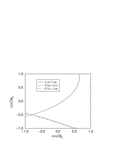
Figure 5: Contours for the “measured values” (39) of the total cross section (solid line), ${\cal P}^{2}/{\cal Q}$ (dashed line), and ${\cal P}^{2}/{\cal Y}$ (dot-dashed line) for $m_{{\chi}^{\pm}_{1}}=95$ GeV [$m_{\tilde{\nu}}=250$ GeV].

The three contour lines meet at a single point $(\cos 2\phi_{L},\cos 2\phi_{R})=(-0.58,-0.48)$ for $m_{\tilde{\nu}}=250$ GeV; note that the sneutrino mass can be determined together with the mixing angles from the “measured values” in eq. (39).

Finally the Lagrangian parameters $M_{2},\mu$ and $\tan\beta$ can be obtained from $m_{\tilde{\chi}^{\pm}_{1}}$, $\cos 2\phi_{L}$ and $\cos 2\phi_{R}$ up to a two-fold ambiguity. It is most transparently achieved by introducing the two auxiliary quantities

$$p=\cot(\phi_{R}-\phi_{L}),\;\;q=\cot(\phi_{R}+\phi_{L})$$ (40)

They are expressed in terms of the measured values $\cos 2\phi_{L}$ and $\cos 2\phi_{R}$ up to a discrete ambiguity due to undetermined signs of $\sin 2\phi_{L}$ and $\sin 2\phi_{R}$

$$p^{2}+q^{2} = \frac{2(\sin^{2}2\phi_{L}+\sin^{2}2\phi_{R})}{(\cos 2\phi_{L}-\cos 2\phi_{R})^{2}}$$

$$pq = \frac{\cos 2\phi_{L}+\cos 2\phi_{R}}{\cos 2\phi_{L}-\cos 2\phi_{R}}$$

$$p^{2}-q^{2} = \frac{4\sin 2\phi_{L}\sin 2\phi_{R}}{(\cos 2\phi_{L}-\cos 2\phi_{R})^{2}}$$ (41)

Solving then eqs. (7) for $\tan\beta$ one finds at most two possible solutions, and using

$$M_{2} = {m_{W}}[(p+q)s_{\beta}-(p-q)c_{\beta}]/\sqrt{2}$$

$$\mu = {m_{W}}[(p-q)s_{\beta}-(p+q)c_{\beta}]/\sqrt{2}$$ (42)

we arrive at $\tan\beta$, $M_{2}$ and $\mu$ up to a two-fold discrete ambiguity. For example, taking the “measured values” from eq. (39), the following results are found [8]

$$[\tan\beta;M_{2},\mu]=\left\{\begin{array}[]{l}[1.06;\;83{\rm GeV},\;-59{\rm GeV}]\\ {}\\ {}[3.33;\;248{\rm GeV},\;123{\rm GeV}]\end{array}\right.$$ (46)

Other sets of “measured values” can lead to a unique solution if the other “possible solution” has a negative $\tan\beta$.

To summarize, from the light chargino pair production, the measurements of the total production cross section and either of the angular correlations among the chargino decay products (${\cal P}^{2}/{\cal Q}$, ${\cal P}^{2}/{\cal Y}$), the physical parameters $m_{\tilde{\chi}^{\pm}_{1}}$, $\cos 2\phi_{L}$ and $\cos 2\phi_{R}$ are determined unambiguously. Then the fundamental parameters $\tan\beta$, $M_{2}$ and $\mu$ are extracted up to a two-fold discrete ambiguity.

If the collider energy is sufficient to produce the two chargino states in pairs, the above ambiguity can be removed [13] by the measurement of the heavier chargino mass. With polarized beams available at the LC, the measurement of the left-right asymmetry $A_{LR}$ can provide [13] an alternative way to extract the mixing angles (or serve as a consistency check).

5 Conclusions

We have discussed how the parameters of the chargino system, the mass of the light chargino $m_{\tilde{\chi}^{\pm}_{1}}$ and the two angles $\phi_{L}$ and $\phi_{R}$, can be extracted from pair production of the light chargino state in $e^{+}e^{-}$ annihilation. In addition to the total production cross section, the measurements of angular correlations among the chargino decay products give rise to two independent observables which can be measured directly despite of the two invisible neutralinos in the final state.

From the chargino mass $m_{\tilde{\chi}^{\pm}_{1}}$ and the two mixing parameters $\cos 2\phi_{L,R}$, the fundamental supersymmetric parameters $\tan\beta$, $M_{2}$ and $\mu$ can be extracted up to at most a two-fold discrete ambiguity. Moreover, from the energy distribution of the final particles in the decay of the chargino, the mass of the lightest neutralino can be measured; this allows us to determine the parameter $M_{1}$ so that also the neutralino mass matrix can be reconstructed in a model-independent way.

Although we only considered real-valued parameters, some of the material presented here goes through unaltered if phases are allowed [8, 13] even though extra information will still be needed to determine those phases.

It should be stressed that the strategy presented here is just at the theoretical level. More realistic simulations of the experimental measurements of physical observables and related errors, including radiative corrections, are needed to assess fully its usefulness. Nevertheless, if the LC and detectors are built and work as expected, no doubt that the actual measurements will be better than anything presented here – provided supersymmetry is discovered!