CERN-TH/99-152
hep-ph/9905550
May 1999

$1S$ and $\overline{\mbox{MS}}$ Bottom Quark Masses from $\Upsilon$ Sum Rules

A.H. Hoang

Theory Division, CERN
CH-1211 Geneva 23, Switzerland

Abstract
The bottom quark $1S$ mass, $M_{b}^{1S}$, is determined using sum rules which relate the masses and the electronic decay widths of the $\Upsilon$ mesons to moments of the vacuum polarization function. The $1S$ mass is defined as half the perturbative mass of a fictitious ${}^{3}\!S_{1}$ bottom-antibottom quark bound state, and is free of the ambiguity of order $\Lambda_{QCD}$ which plagues the pole mass definition. Compared to an earlier analysis by the same author, which had been carried out in the pole mass scheme, the $1S$ mass scheme leads to a much better behaved perturbative series of the moments, smaller uncertainties in the mass extraction and to a reduced correlation of the mass and the strong coupling. We arrive at $M_{b}^{1S}=4.71\pm 0.03$ GeV taking $\alpha_{s}(M_{Z})=0.118\pm 0.004$ as an input. From that we determine the $\overline{\mbox{MS}}$ mass as $\overline{m}_{b}(\overline{m}_{b})=4.20\pm 0.06$ GeV. The error in $\overline{m}_{b}(\overline{m}_{b})$ can be reduced if the three-loop corrections to the relation of pole and $\overline{\mbox{MS}}$ mass are known and if the error in the strong coupling is decreased.
PACS numbers: 14.65.Fy, 13.20.Gd, 13.20.Gv.

1 Introduction

The determination of the Cabibbo-Kobayashi-Maskawa (CKM) matrix elements is one of the main goals of future $B$ physics experiments. A sufficiently accurate determination of the size of the CKM matrix elements and their relative phases will lead to a better understanding of the origin of CP violation, the structure of the weak interaction, and, possibly, to the establishment of physics beyond the Standard Model. For the extraction of the CKM matrix elements from inclusive $B$ decay rates, particularly of $V_{cb}$ from the semileptonic decays into $D$ mesons, an accurate and precise knowledge of the bottom quark mass is desirable due to the strong dependence of the total decay rate on the bottom quark mass parameter.

Non-relativistic sum rules for the masses and electronic decay widths of $\Upsilon$ mesons, bottom-antibottom quark bound states having photonic quantum numbers, are an ideal tool to determine the bottom quark mass: using causality and global duality arguments one can relate integrals over the total cross section for the production of hadrons containing a bottom-antibottom quark pair in $e^{+}e^{-}$ collisions to derivatives of the vacuum polarization function of bottom quark currents at zero-momentum transfer. For a particular range of numbers of derivatives the moments are saturated by the experimental data on the $\Upsilon$ mesons and, at the same time, can be calculated reliably using perturbative QCD in the non-relativistic expansion. Because the moments have, for dimensional reasons, a strong dependence on the bottom quark mass, these sum rules can be used to determine the bottom quark mass to high precision. Within the last few years there have been several analyses at NLO and NNLO in the non-relativistic expansion, where it has been attempted to extract the bottom quark pole mass from these sum rules. [1, 2, 3, 4, 5] The results for the pole mass given in these analyses vary rather strongly in their central values and their precision. This reflects the fact that the concept of the pole mass is ambiguous to an amount of order the typical hadronization scale $\Lambda_{QCD}$ [7, 8]. From a technical point of view the large variations in the extracted pole mass values arise from large correlations to the value of the strong coupling $\alpha_{s}$, the theoretical uncertainties coming from large NNLO corrections to the moments, a strong residual dependence on the renormalization scale, and a different interpretation and treatment of these sources of uncertainties in the various analyses. From a conceptual point of view at least part of the former issues can be traced back to the fact that in the pole mass scheme the theoretical expressions for the moments are sensitive to scales which are below the scales characteristic to the non-relativistic bottom-antibottom quark dynamics encoded in the moments. This sensitivity to low scales, which becomes stronger at higher orders of perturbation theory and which is called the “renormalon” problem of the pole mass definition, is an artifact of the pole mass scheme, and does not exist if a mass definition is employed which is not ambiguous to an amount of order $\Lambda_{QCD}$ [9, 10]. Such mass definitions are referred to as “short-distance” masses. (Short-distance masses can still have ambiguities of order $\Lambda_{QCD}^{2}$ divided by the heavy quark mass.) In general, these mass definitions have a nicely behaved perturbative relation to the $\overline{\mbox{MS}}$ mass. This means that the perturbative relation between the short-distance masses and the $\overline{\mbox{MS}}$ mass can be expected to be convergent for all practical purposes (i.e. as long as we only deal with a few low orders of perturbation theory). However, not any short-distance mass is equally well adapted to improve the situation for the $\Upsilon$ sum rules because the correlations to the strong coupling and the strong dependence on the renormalization scale observed in the pole mass scheme already exist in the leading order theoretical expressions for the moments and are therefore not related to the problem of an increased infrared sensitivity. Thus, it is advantageous to use a specialised short-distance mass for the mass extraction from the $\Upsilon$ sum rules, which eliminates, as much as possible, correlations and dependences to other parameters and which stabilises the perturbative expansion of the moments. Such a specialised short-distance mass can be either used as a mass definition in its own right, or, in a second step, related to other short-distance masses like the $\overline{\mbox{MS}}$ mass, which can be regarded as a specialised short-distance mass designed for high energy processes. In this step a part of the correlations to the strong coupling are expected to come back. However, correlations to other parameters like renormalization scales are eliminated, which can lead to a reduction of uncertainties. In addition, the perturbative relations between short-distance masses is well convergent and possible sources of correlations which arise in these relations can be easily identified.

In this paper we extract the $1S$ bottom quark mass from the $\Upsilon$ sum rules based on the theoretical expressions of the moments which we have calculated analytically at next-to-next-to-leading order (NNLO) in the pole mass scheme in a previous publication [4]. In the $1S$ scheme the bottom quark mass is defined as half the perturbative mass of a colour singlet bottom-antibottom quark $J^{PC}=1^{--}$, ${}^{3}\!S_{1}$ bound state. The $1S$ mass is a short-distance mass and has been used previously to parameterise inclusive $B$ mesons decays leading to a considerable reduction of the perturbative corrections. [11, 12] In the $1S$ mass scheme we find a reduction in the size of the large NNLO corrections to the theoretical moments observed in the pole mass scheme, and a much weaker dependence of the moments on $\alpha_{s}$ and the renormalization scale governing the non-relativistic bottom-antibottom quark dynamics. This results in a weak correlation of the $1S$ mass to the value of the strong coupling and to much smaller uncertainties in the mass determination compared to our earlier analysis in the pole scheme ($M_{b}^{1S}=4.71\pm 0.03$ GeV in this work versus $M_{b}^{pole}=4.9\pm 0.1$ GeV in Ref. [4] if $\alpha_{s}(M_{Z})=0.118\pm 0.004$ is taken as input) using exactly the same statistical analysis and the same way to treat theoretical uncertainties.

By construction, the $1S$ mass is half the perturbative contribution of the $\Upsilon(1S)$ meson mass ($M_{\Upsilon(1S)}=9460.37\pm 0.21$ MeV [13]). In Refs. [11, 12] this relation has been used explicitly, and an uncertainty of $\pm 50$ MeV has been assigned to the value of $M_{b}^{1S}$ based on conservative general arguments to estimate the size of non-perturbative effects in the $\Upsilon(1S)$ mass. In this work this relation is not used and $M_{b}^{1S}$ is treated as a fictitious mass parameter which is determined solely from the sum rule analysis. The close proximity of $M_{b}^{1S}$ determined in this work and $M_{\Upsilon(1S)}/2=4.730$ GeV is non-trivial because higher radial $\Upsilon$ meson excitations and the $b\bar{b}$ continuum have a significant contribution to the sum rule. Thus the analysis in this work provides an independent quantitative cross check of the arguments about the size of non-perturbative effects in the $\Upsilon(1S)$ mass made in Refs. [11, 12].

The program of this paper is as follows: in Sec. 2 we introduce the $1S$ mass. In Sec. 3 we briefly review the $\Upsilon$ sum rules and discuss how the analytic results obtained in Ref. [4] in the pole scheme are modified in the $1S$ mass scheme. In Sec. 4 the statistical analysis is explained and the results of the determination of the $1S$ bottom quark mass are shown. In Sec. 5 we discuss the upsilon expansion [11, 12] which is needed to relate the $1S$ mass to other short-distance mass definitions, and we determine the $\overline{\mbox{MS}}$ mass. In Sec. 6 we determine the value of other recently proposed specialised short-distance masses which can be used in the $\Upsilon$ sum rules, and Sec. 7 contains the conclusions.

2 The $1S$ Bottom Quark Mass

The $1S$ bottom quark mass is defined as half the perturbative mass of a $J^{PC}=1^{--}$, ${}^{3}\!S_{1}$ bottomonium ground state. Expressed in terms of the pole mass the $1S$ mass at NNLO in the non-relativistic expansion reads ($a_{s}=\alpha_{s}(\mu)$), [14, 5]

$$M_{b}^{1S} = M_{b}^{pole}\,\bigg{[}\,1\,-\,\epsilon\,\Delta^{\mbox{\tiny LO}}(a_{s})\,-\,\epsilon^{2}\,\Delta^{\mbox{\tiny NLO}}(M_{b}^{pole},a_{s},\mu)\,-\,\epsilon^{3}\,\Delta^{\mbox{\tiny NNLO}}(M_{b}^{pole},a_{s},\mu)\,\bigg{]}\,,$$ (1)

where

$$\Delta^{\mbox{\tiny LO}} = \frac{C_{F}^{2}\,a_{s}^{2}}{8}\,,$$ (2)

$$\Delta^{\mbox{\tiny NLO}} = \frac{C_{F}^{2}\,a_{s}^{2}}{8}\,\Big{(}\frac{a_{s}}{\pi}\Big{)}\,\bigg{[}\,\beta_{0}\,\bigg{(}L+1\,\bigg{)}+\frac{a_{1}}{2}\,\bigg{]}\,,$$ (3)

$$\Delta^{\mbox{\tiny NNLO}} = \frac{C_{F}^{2}\,a_{s}^{2}}{8}\,\Big{(}\frac{a_{s}}{\pi}\Big{)}^{2}\,\bigg{[}\,\beta_{0}^{2}\,\bigg{(}\,\frac{3}{4}L^{2}+L+\frac{\zeta_{3}}{2}+\frac{\pi^{2}}{24}+\frac{1}{4}\,\bigg{)}+\beta_{0}\,\frac{a_{1}}{2}\,\bigg{(}\,\frac{3}{2}\,L+1\,\bigg{)}$$ (4)

$$\hskip 42.67912pt+\frac{\beta_{1}}{4}\,\bigg{(}\,L+1\,\bigg{)}+\frac{a_{1}^{2}}{16}+\frac{a_{2}}{8}+\bigg{(}\,C_{A}-\frac{C_{F}}{48}\,\bigg{)}\,C_{F}\pi^{2}\,\bigg{]}\,,$$

$$L \equiv \ln\Big{(}\frac{\mu}{C_{F}\,a_{s}\,M_{b}^{pole}}\Big{)}\,,$$ (5)

and ($n_{l}=4$)

$$\beta_{0} = \frac{11}{3}\,C_{A}-\frac{4}{3}\,T\,n_{l}\,,$$

$$\beta_{1} = \frac{34}{3}\,C_{A}^{2}-\frac{20}{3}C_{A}\,T\,n_{l}-4\,C_{F}\,T\,n_{l}\,,$$

$$a_{1} = \frac{31}{9}\,C_{A}-\frac{20}{9}\,T\,n_{l}\,,$$

$$a_{2} = \bigg{(}\,\frac{4343}{162}+4\,\pi^{2}-\frac{\pi^{4}}{4}+\frac{22}{3}\,\zeta_{3}\,\bigg{)}\,C_{A}^{2}-\bigg{(}\,\frac{1798}{81}+\frac{56}{3}\,\zeta_{3}\,\bigg{)}\,C_{A}\,T\,n_{l}$$ (6)

$$-\bigg{(}\,\frac{55}{3}-16\,\zeta_{3}\,\bigg{)}\,C_{F}\,T\,n_{l}+\bigg{(}\,\frac{20}{9}\,T\,n_{l}\,\bigg{)}^{2}\,.$$

The constants $\beta_{0}$ and $\beta_{1}$ are the one- and two-loop coefficients of the QCD beta function and the constants $a_{1}$ [15, 16] and $a_{2}$ [17, 18] the non-logarithmic one- and two-loop corrections to the static colour-singlet heavy quark potential in the pole mass scheme, $V^{Coul}$. The charm quark is treated as massless. In Eq. (1) we have labelled the contributions at LO, NLO and NNLO in the non-relativistic expansion by powers $\epsilon$, $\epsilon^{2}$ and $\epsilon^{3}$, respectively, of the auxiliary parameter $\epsilon=1$. The expansion in terms of the parameter $\epsilon$ is called the upsilon expansion [11, 12] and will be relevant when the $1S$ is related to the $\overline{\mbox{MS}}$ mass. We will come back to this issue in Sec. 5

In the framework of the non-relativistic power counting scheme $\Delta_{LO}$, $\Delta_{NLO}$ and $\Delta_{NNLO}$ are of order $v^{2},v^{3}$ and $v^{4}$ respectively. In order to implement the $1S$ mass into the analytic expressions for the moments in the pole mass scheme we have to invert relation (1) in the non-relativistic framework,

$$M_{b}^{pole} = M_{b}^{1S}\,\bigg{\{}\,1\,+\,\Delta^{LO}(a_{s})\,+\,\Delta^{NLO}(M_{b}^{1S},a_{s},\mu)$$ (7)

$$\mbox{\hskip 28.45274pt}\,+\,\bigg{[}\,\Delta^{NNLO}(M_{b}^{1S},a_{s},\mu)+\Big{(}\Delta^{LO}(a_{s})\Big{)}^{2}\,\bigg{]}\,\bigg{\}}\,.$$

The terms in the brackets on the RHS of Eq. (7) represent the NNLO contributions. We would like to emphasise again that $M_{b}^{1S}$ is a short-distance mass because it does not suffer from the ambiguity of order $\Lambda_{QCD}$ like the pole mass. This is because the $1S$ mass contains, by construction, the half of the total static energy $\langle 2M_{b}^{pole}+V^{Coul}\rangle$ which can be proven to be ambiguity-free at order $\Lambda_{QCD}$. [9, 10]

3 The $\Upsilon$ Sum Rules

In this section we briefly review the basic concepts involved in the $\Upsilon$ meson sum rules. We outline the calculation of the moments in the pole mass scheme which has been carried out in Ref. [4], and we describe how the moments have to be modified in the $1S$ scheme. We will not present any details on the original computations carried out in the pole mass scheme and refer the interested reader to Ref. [4].

The sum rules for the $\Upsilon$ mesons start from the correlator of two electromagnetic currents of bottom quarks at momentum transfer $q$,

$$\Pi_{\mu\nu}(q)\,=\,-\,i\int\!{\rm d}x\,e^{i\,q.x}\,\langle\,0\,|\,T\,j^{b}_{\mu}(x)\,j^{b}_{\nu}(0)\,|\,0\,\rangle\,,$$ (8)

where

$$j^{b}_{\mu}(x)\,=\bar{b}(x)\,\gamma_{\mu}\,b(x)\,,$$ (9)

and the symbol $b$ denotes the bottom quark Dirac field. The $n$-th moment $P_{n}$ of the vacuum polarization function is defined as

$$P_{n}\,\equiv\,\frac{4\,\pi^{2}\,Q_{b}^{2}}{n!\,q^{2}}\,\bigg{(}\frac{d}{dq^{2}}\bigg{)}^{n}\,\Pi_{\mu}^{\,\,\,\mu}(q)\bigg{|}_{q^{2}=0}\,,$$ (10)

where $Q_{b}=-1/3$ is the electric charge of the bottom quark. Due to causality the n-th moment $P_{n}$ can also be written as a dispersion integral

$$P_{n}\,=\,\int\limits^{\infty}_{\sqrt{s}_{min}}\frac{ds}{s^{n+1}}\,R(s)\,,$$ (11)

where

$$R(s)\,=\,\frac{\sigma(e^{+}e^{-}\to\gamma^{*}\to\mbox{``$b\bar{b}$''})}{\sigma_{pt}}$$ (12)

is the total photon mediated cross section of bottom quark-antiquark production in $e^{+}e^{-}$ annihilation normalised to the point cross section $\sigma_{pt}\equiv 4\pi\alpha^{2}/3s$, and $s$ the square of the centre-of-mass energy. The lower limit of the integration in Eq. (11) is set by the mass of the lowest lying resonance. Assuming global duality the moments $P_{n}$ can be either calculated from experimental data on $R$ or theoretically using perturbative QCD.

The experimental moments $P_{n}^{ex}$ are determined using latest data on the $\Upsilon$ meson masses, $M_{\Upsilon(nS)}$, and electronic decay widths, $\Gamma_{\Upsilon(nS)}$, for $n=1,\ldots,6$. The formula for the experimental moments used in this work reads

$$P_{n}^{ex} = \frac{9\,\pi}{\tilde{\alpha}^{2}_{em}}\,\sum\limits_{k=1}^{6}\,\frac{\Gamma_{\Upsilon(kS)}}{M_{\Upsilon(k)}^{2n+1}}\,+\,\int\limits_{\sqrt{s}_{B\bar{B}}}^{\infty}\frac{ds}{s^{n+1}}\,r_{cont}(s)\,.$$ (13)

and is based on the narrow width approximation for the known $\Upsilon$ resonances. $\tilde{\alpha}_{em}$ is the electromagnetic coupling at the scale $10$ GeV. Because the difference in the electromagnetic coupling for the different $\Upsilon$ masses is negligible we chose $10$ GeV as the scale of the electromagnetic coupling for all resonances. The continuum cross section above the $B\bar{B}$ threshold is approximated by the constant $r_{c}=1/3$, which is equal to the born cross section for $s\to\infty$, assuming a $50\%$ uncertainty

$$r_{cont}(s)=r_{c}\,(1\pm 0.5)\,.$$ (14)

For $n\geq 4$ the continuum contribution is already sufficiently suppressed that a more detailed description is not needed. For a compilation of all experimental numbers used in this work see Tab. 1.

$nS$	$1S$	$2S$	$3S$
$M_{nS}/[\mbox{GeV}]$	$9.460$	$10.023$	$10.355$
$\Gamma_{nS}/[\mbox{keV}]$	$1.32\pm 0.04\pm 0.03$	$0.52\pm 0.03\pm 0.01$	$0.48\pm 0.03\pm 0.03$
$nS$	$4S$	$5S$	$6S$
$M_{nS}/[\mbox{GeV}]$	$10.58$	$10.87$	$11.02$
$\Gamma_{nS}/[\mbox{keV}]$	$0.25\pm 0.03\pm 0.01$	$0.31\pm 0.05\pm 0.07$	$0.13\pm 0.03\pm$ 0.03
$\tilde{\alpha}_{em}^{-1}=\alpha_{em}^{-1}(10$ GeV$)=131.8(1\pm 0.005)\,,\quad(\sqrt{s})_{B\bar{B}}=2\times 5.279$ GeV

Table 1: The experimental numbers for the $\Upsilon$ masses and electronic decay widths used for the calculation of the experimental moments $P_{n}^{ex}$. For the widths the first error is statistical and the second systematical. The errors for the partial widths of $\Upsilon_{1S}$ and $\Upsilon_{2S}$ are taken from Ref. [19]. All the other errors are estimated from the numbers presented in Ref. [13]. The small errors in the $\Upsilon$ masses and the $B\bar{B}$ threshold $(\sqrt{s})_{B\bar{B}}$ are neglected.

A reliable computation of the theoretically moments based on perturbative QCD is only possible if the effective energy range contributing to the integration in Eq. (11) is sufficiently larger than $\Lambda_{QCD}\sim{\cal{O}}(200-300~{}\mbox{MeV})$ [20]. For large values of $n$ one can show that the size of this energy range is of order $M_{b}/n$. This means that $n$ should be chosen sufficiently smaller than $15-20$. To suppress systematic theoretical uncertainties as much as possible we take $n_{max}=10$ as the maximal allowed value for $n$. However, it is also desirable to choose $n$ as large as possible in order to suppress the contribution from the $b\bar{b}$ continuum to $R(s)$ above the $B\bar{B}$ threshold, which is rather poorly known experimentally. In other words, one has to choose $n$ large enough that the bottom-antibottom quark dynamics encoded in the moments $P_{n}$ is non-relativistic. Because the effective size of the energy range contributing to the $n$-th moment is of order $M_{b}/n$, the mean centre-of-mass velocity of the bottom quarks in the $n$-th moment is of order

$$v\,\sim\,\alpha_{s}\,\sim\,\frac{1}{\sqrt{n}}\,,$$ (15)

where $v\sim\alpha_{s}$ is characteristic for perturbative non-relativistic quark-antiquark systems. In our analysis we choose $n_{min}=4$ as the minimal value of $n$ to ensure the dominance of the non-relativistic dynamics in the moments. For the values of $n$ employed in our analysis the non-perturbative contributions coming from the gluon condensate are at the per-mill level and negligible. [1]

In Ref. [4] we have used non-relativistic QCD (NRQCD) as formulated in Ref. [21] to determine the theoretical moments $P_{n}^{th}$ in the pole mass scheme at NNLO in the non-relativistic expansion, which included all corrections up to order $1/n$, $\alpha_{s}/\sqrt{n}$ and $\alpha_{s}^{2}$ with respect to the expressions which are leading order in the non-relativistic expansion. Taking into account the power counting shown in Eq. (15) the dispersion integration for the theoretical moments $P_{n}^{th}$ at NNLO takes the form

$$P_{n}^{th}\,=\,\frac{1}{4^{n}\,(M_{b}^{pole})^{2n}}\,\int\limits_{E_{\rm bind}}^{\infty}\frac{dE}{M_{b}^{pole}}\,\exp\bigg{\{}\,-\frac{E}{M_{b}^{pole}}\,n\,\bigg{\}}\,\bigg{(}\,1-\frac{E}{2\,M_{b}^{pole}}+\frac{E^{2}}{4\,(M_{b}^{pole})^{2}}\,n\,\bigg{)}\,R_{\mbox{\tiny NNLO}}^{\mbox{\tiny thr}}(E)\,,$$ (16)

where $E\equiv\sqrt{s}-2M_{b}^{pole}$ and $E_{\rm bind}$ is the binding energy of the lowest lying resonance, i.e. $E_{\rm bind}=2(M_{b}^{1S}-M_{b}^{pole})$. The exponential form of the LO non-relativistic contribution to the energy integration has to be chosen because $E$ scales like $v^{2}\sim 1/n$. The result for the theoretical moments at NNLO can be cast into the form

$$P_{n}^{th} = \frac{3\,N_{c}\,Q_{b}^{2}\,\sqrt{\pi}}{4^{n+1}\,(M_{b}^{pole})^{2n}\,n^{3/2}}\,\bigg{\{}\,C_{1}\Big{(}\frac{\mu_{\rm hard}}{M_{b}^{pole}},\frac{\mu_{\rm fac}}{M_{b}^{pole}},\alpha_{s}(\mu_{\rm hard})\Big{)}\,\varrho_{n,1}\Big{(}\frac{\mu_{\rm soft}}{M_{b}^{pole}},\frac{\mu_{\rm fac}}{M_{b}^{pole}},\alpha_{s}(\mu_{\rm soft})\Big{)}$$ (17)

$$\mbox{\hskip 113.81102pt}+\,\varrho_{n,2}\Big{(}\alpha_{s}(\mu_{\rm soft})\Big{)}\,\bigg{\}}\,,$$

where $\varrho_{n,1}$ describes the contribution to the moments coming from the dominant non-relativistic current correlator involving two dimension three ${}^{3}\!S_{1}$ NRQCD currents, and $\varrho_{n,2}$ the contribution coming from the NNLO current correlator involving one dimension three and one dimension five ${}^{3}\!S_{1}$ NRQCD current. $C_{1}$ contains the short-distance corrections to the dimension three currents up to order ${\cal{O}}(\alpha_{s}^{2})$. The corresponding short-distance correction to $\varrho_{n,2}$ is not needed because the latter is already of NNLO. In Eq. (17) we have indicated the dependence of the moments on the various renormalization scales used in Ref. [4]. $\mu_{\rm soft}$ is the renormalization scale of the strong coupling governing the non-relativistic dynamics and $\mu_{\rm hard}$ the scale of the strong coupling in the short-distance coefficient $C_{1}$. The scale $\mu_{\rm fac}$ is the factorisation scale which separates non-relativistic and short-distance momenta. The three scales arise in the calculation of Ref. [4] as a consequence of the use of a cutoff-like regularization for the UV divergences which arise in NRQCD Feynman diagrams, while the strong coupling is renormalised in the $\overline{\mbox{MS}}$ scheme. Formally the moments are invariant under changes of these scales at NNLO. From the numerical point of view, however, they are not, because the dependence on the scales, in particular the soft scale, only cancels partially at finite order of perturbation theory. In the statistical analysis for the bottom mass determination all three scales are varied independently in order to estimate theoretical uncertainties. Eq. (17) also displays the dependence on the pole mass. The short-distance factor $C_{1}$ and $\varrho_{n,1}$ only depend on the pole mass through the logarithm of the ratios of the renormalization scales and the pole mass, which originate from the running of the strong coupling and the NRQCD UV divergences. The latter dependences only arise at NLO and NNLO and do not lead to any modifications in the $1S$ scheme because the difference between $1S$ and pole mass is of order $v^{2}\sim\alpha_{s}^{2}\sim 1/n$ in the non-relativistic expansion. The most important pole mass dependence is the overall factor $(M_{b}^{pole})^{-2n}$. In the $1S$ scheme this factor reads

$$\frac{1}{(M_{b}^{pole})^{2n}}\,=\,\frac{1}{(M_{b}^{1S})^{2n}}\,\exp\Big{(}-2\,n\,\Delta^{\mbox{\tiny LO}}(\alpha_{s}(\mu_{\rm soft}))\Big{)}\,\bigg{\{}\,1-2\,n\,\Delta^{\mbox{\tiny NLO}}(M_{b}^{1S},\alpha_{s}(\mu_{\rm soft}),\mu_{\rm soft})$$

$$\mbox{}+\,n\bigg{[}\Big{(}\Delta^{\mbox{\tiny LO}}(\alpha_{s}(\mu_{\rm soft}))\Big{)}^{2}-2\Delta^{\mbox{\tiny NNLO}}(M_{b}^{1S},\alpha_{s}(\mu_{\rm soft}),\mu_{\rm soft})+2n\Big{(}\Delta^{\mbox{\tiny NLO}}(M_{b}^{1S},\alpha_{s}(\mu_{\rm soft}),\mu_{\rm soft})\Big{)}^{2}\bigg{]}\bigg{\}}$$

at NNLO in the non-relativistic expansion using the relation given in Eq. (7).

Moment		$M_{b}^{1S}(M_{b}^{pole})/[GeV]$			$\alpha_{s}(M_{Z})$
		$4.6$	$4.8$	$5.0$	$0.11$	$0.12$	$0.13$
$P_{4}^{th}$$/$	$[10^{-8}\,\mbox{GeV}^{-8}]$	$0.27$($0.39$)	$0.19$($0.28$)	$0.14$($0.20$)	$0.17$($0.22$)	$0.20$($0.30$)	$0.26$($0.46$)
$P_{6}^{th}$$/$	$[10^{-12}\,\mbox{GeV}^{-12}]$	$0.28$($0.47$)	$0.17$($0.29$)	$0.11$($0.18$)	$0.14$($0.21$)	$0.18$($0.31$)	$0.24$($0.54$)
$P_{8}^{th}$$/$	$[10^{-16}\,\mbox{GeV}^{-16}]$	$0.33$($0.64$)	$0.17$($0.33$)	$0.09$($0.17$)	$0.14$($0.22$)	$0.18$($0.36$)	$0.25$($0.70$)
$P_{10}^{th}$$/$	$[10^{-20}\,\mbox{GeV}^{-20}]$	$0.41$($0.90$)	$0.18$($0.39$)	$0.08$($0.17$)	$0.14$($0.25$)	$0.19$($0.44$)	$0.27$($0.94$)
$P_{20}^{th}$$/$	$[10^{-40}\,\mbox{GeV}^{-40}]$	$1.64$($6.85$)	$0.30$($1.26$)	$0.06$($0.25$)	$0.22$($0.63$)	$0.33$($1.52$)	$0.53$($4.72$)
		$\alpha_{s}(M_{Z})=0.118$			$M_{b}^{1S}=4.8$ GeV
					($M_{b}^{pole}=4.8$ GeV)
		$\mu_{\rm soft}=2.5\,\mbox{GeV}\,,\quad\mu_{\rm hard}=\mu_{\rm fac}=5$ GeV

Table 2: The theoretical moments $P_{n}^{th}$ at NNLO in the $1S$ (pole) mass scheme for $n=4,6,8,10,20$ and fixed $\mu_{\rm soft}=2.5$ GeV and $\mu_{\rm hard}=\mu_{\rm fac}=5$ GeV for various values of $M_{b}^{1S}$ ($M_{b}^{pole}$) and $\alpha_{s}(M_{z})$. The two-loop running has been employed for the strong coupling. The values for $P_{n}^{th}$ in the pole mass scheme are slightly different from the numbers shown in Ref. [4] because of the correction in $a_{2}$.

Moment		$\mu_{\rm soft}/[\mbox{GeV}]$		$\mu_{\rm hard}/[\mbox{GeV}]$		$\mu_{\rm fac}/[\mbox{GeV}]$
		$1.5$	$3.5$	$2.5$	$10.0$	$2.5$	$10.0$
$P_{4}^{th}$$/$	$[10^{-8}\,\mbox{GeV}^{-8}]$	$0.33$($0.51$)	$0.17$($0.23$)	$0.17$($0.25$)	$0.21$($0.30$)	$0.21$($0.31$)	$0.16$($0.22$)
$P_{6}^{th}$$/$	$[10^{-12}\,\mbox{GeV}^{-12}]$	$0.31$($0.57$)	$0.14$($0.22$)	$0.15$($0.26$)	$0.19$($0.31$)	$0.19$($0.33$)	$0.14$($0.22$)
$P_{8}^{th}$$/$	$[10^{-16}\,\mbox{GeV}^{-16}]$	$0.31$($0.70$)	$0.14$($0.25$)	$0.15$($0.29$)	$0.18$($0.35$)	$0.19$($0.38$)	$0.14$($0.25$)
$P_{10}^{th}$$/$	$[10^{-20}\,\mbox{GeV}^{-20}]$	$0.34$($0.89$)	$0.14$($0.28$)	$0.16$($0.35$)	$0.19$($0.42$)	$0.20$($0.46$)	$0.14$($0.30$)
$P_{20}^{th}$$/$	$[10^{-40}\,\mbox{GeV}^{-40}]$	$0.63$($3.75$)	$0.24$($0.80$)	$0.27$($1.12$)	$0.33$($1.36$)	$0.34$($1.54$)	$0.24$($0.92$)
		$\mu_{\rm hard}=5$ GeV		$\mu_{\rm soft}=2.5$ GeV		$\mu_{\rm soft}=2.5$ GeV
		$\mu_{\rm fac}=5$ GeV		$\mu_{\rm fac}=5$ GeV		$\mu_{\rm hard}=5$ GeV

Table 3: The theoretical moments $P_{n}^{th}$ for $n=4,6,8,10,20$ and fixed $\alpha_{s}(M_{Z})=0.118$ and $M_{b}^{1S}=4.8$ GeV ($M_{b}^{pole}=4.8$ GeV) for various choices of the renormalization scales $\mu_{\rm soft}$, $\mu_{\rm hard}$ and $\mu_{\rm fac}$. The two-loop running has been employed for the strong coupling. The values for $P_{n}^{th}$ in the pole mass scheme are slightly different from the numbers shown in Ref. [4] because of the correction in $a_{2}$.

Moment	$M_{b}^{1S}(M_{b}^{pole})/[GeV]$			$\alpha_{s}(M_{Z})$
	$4.6$	$4.8$	$5.0$	$0.11$	$0.12$	$0.13$
$P_{4,\mbox{\tiny LO}}^{th}$	$0.35$($0.40$)	$0.25$($0.29$)	$0.18$($0.21$)	$0.21$($0.23$)	$0.26$($0.31$)	$0.35$($0.43$)
$P_{4,\mbox{\tiny NLO}}^{th}$	$0.19$($0.26$)	$0.13$($0.18$)	$0.09$($0.13$)	$0.13$($0.16$)	$0.13$($0.18$)	$0.12$($0.23$)
$P_{4,\mbox{\tiny NNLO}}^{th}$	$0.27$($0.39$)	$0.19$($0.28$)	$0.14$($0.20$)	$0.17$($0.22$)	$0.20$($0.30$)	$0.26$($0.46$)
$P_{10,\mbox{\tiny LO}}^{th}$	$0.45$($0.62$)	$0.19$($0.27$)	$0.09$($0.12$)	$0.15$($0.19$)	$0.21$($0.29$)	$0.30$($0.53$)
$P_{10,\mbox{\tiny NLO}}^{th}$	$0.26$($0.53$)	$0.11$($0.22$)	$0.05$($0.10$)	$0.10$($0.16$)	$0.11$($0.24$)	$0.12$($0.43$)
$P_{10,\mbox{\tiny NNLO}}^{th}$	$0.41$($0.90$)	$0.18$($0.39$)	$0.08$($0.17$)	$0.14$($0.25$)	$0.19$($0.44$)	$0.27$($0.94$)
	$\alpha_{s}(M_{Z})=0.118$			$M_{b}^{1S}=4.8$ GeV
				($M_{b}^{pole}=4.8$ GeV)
	$\mu_{\rm soft}=2.5\,\mbox{GeV}\,,\quad\mu_{\rm hard}=\mu_{\rm fac}=5$ GeV

Table 4: The theoretical moments $P_{4}^{th}$ and $P_{10}^{th}$ at LO, NLO and NNLO for fixed $\mu_{\rm soft}=2.5$ GeV and $\mu_{\rm hard}=\mu_{\rm fac}=5$ GeV for various values of $M_{b}^{1S}$ ($M_{b}^{pole}$) and $\alpha_{s}(M_{Z})$ in the $1S$ (pole) mass scheme. The two-loop running has been employed for the strong coupling. The values of $P_{4}^{th}$ and $P_{10}^{th}$ are given in units of $10^{-8}\,\mbox{GeV}^{-8}$ and $10^{-20}\,\mbox{GeV}^{-20}$, respectively.

$n$	$4$	$6$	$8$	$10$
$P_{n}^{ex}/[10^{-2n}\,\mbox{GeV}^{-2n}]$	$0.22$	$0.21$	$0.23$	$0.26$
$(P_{n}^{ex})^{\Upsilon(1S)}/[10^{-2n}\,\mbox{GeV}^{-2n}]$	$0.11$	$0.13$	$0.17$	$0.21$
$(P_{n}^{ex})^{\Upsilon(1S)}/P_{n}^{ex}$	$0.48$	$0.62$	$0.72$	$0.79$

Table 5: The experimental moments, $P_{n}^{ex}$, the contribution of the $\Upsilon(1S)$ to the experimental moments, $(P_{n}^{ex})^{\Upsilon(1S)}$, and the ratio $(P_{n}^{ex})^{\Upsilon(1S)}/P_{n}^{ex}$ for $n=4,6,8,10$.

Because the $1S$ mass is defined purely from the non-relativistic dynamics, the soft scale has to be employed in Eq. (LABEL:finalfactor). Thus, the transition to the $1S$ mass scheme leads to a simple rescaling of the theoretical moments. We emphasise that the expression in Eq. (LABEL:finalfactor) must be expanded consistently up to NNLO in the non-relativistic expansion together with the LO, NLO and NNLO contributions of $\varrho_{n,1}$ and with $\varrho_{n,2}$ in order to achieve a proper cancellation of the correlations and the large NNLO corrections which are present in the pole mass scheme. Like in Ref. [4] we keep the short-distance coefficient $C_{1}$ in factorized form.

Comparing Eqs. (LABEL:finalfactor) and (16) we can easily see that the $1S$ scheme represents the most natural scheme one can use to avoid correlations and large corrections because it reduces the contribution from the lowest lying bottom-antibottom quark resonance, which represents the most important part of theoretical moments at large values of $n$.

Before we turn to the statistical analysis it is quite interesting to study the impact of the transition to the $1S$ scheme on the theoretical moments. In Tab. 2 we have displayed the values of $P_{n}^{th}$ in the $1S$ (pole) scheme for $n=4,6,8,10,20$ and for various values of $M_{b}^{1S}$ ($M_{b}^{pole}$) and $\alpha_{s}(M_{z})$ while the renormalization scales are fixed to $\mu_{\rm soft}=2.5$ GeV and $\mu_{\rm hard}=\mu_{\rm fac}=5$ GeV. The numbers in Tab. 2 show that the dependence of the moments on the mass is quite strong in the $1S$ as well as in the pole mass scheme. However, in the $1S$ scheme the variation with respect to changes in the strong coupling is much weaker, in particular for larger values of $n$. To illustrate this we have also displayed the moments for $n=20$, although this value it too high for the practical application. From this we can expect that the extracted values for $M_{b}^{1S}$ are less strongly correlated to the strong coupling than the pole mass values obtained in Ref. [4]. This feature, however, will also make an independent determination of a precise value for the strong coupling from the $\Upsilon$ sum rules impossible in the $1S$ scheme, as we show in the next section.

In Tab. 3 the theoretical moments are displayed for $n=4,6,8,10,20$ for different choices of $\mu_{\rm soft}$, $\mu_{\rm hard}$ and $\mu_{\rm fac}$ for $\alpha_{s}(M_{Z})=0.118$ and $M_{b}^{1S}=4.8$ GeV ($M_{b}^{pole}=4.8$ GeV) in the $1S$ (pole) mass scheme. As expected from the weak dependence of the moments in the $1S$ scheme on the strong coupling, we also find that the dependence of the moments on the soft scale is weaker in the $1S$ scheme, in particular for larger values of $n$. In the $1S$ scheme there is also some stabilization with respect to variations of the factorisation scale. The dependence of the moments on the hard scale, on the other hand, is comparable in both schemes. This is expected because in the transition from the pole to the $1S$ scheme only non-relativistic contributions are modified. Because the variation of the moments with respect to the renormalization scales is used as an instrument to estimate theoretical uncertainties in the mass extraction we can expect smaller uncertainties in the $1S$ mass extraction compared to the results shown in Ref. [4].

In Tab. 4 the theoretical moment $P_{4}^{th}$ and $P_{10}^{th}$ are displayed at LO, NLO and NNLO in the $1S$ (pole) scheme. Whereas in the pole mass scheme the NNLO corrections are all of the same size or even larger than the NLO corrections, they are significantly smaller in the $1S$ scheme. This illustrates the improvement of the perturbative behaviour of the theoretical moments if the $1S$ mass scheme is employed. We emphasise, however, that even in the $1S$ scheme the NNLO corrections are not per se small, particularly for large values of $n$. We believe that this is not a point of concern, because of the extreme dependence of the moments on the bottom quark mass, particularly for large values of $n$. It is the behavior of the results for the mass extracted from the theoretical moments which should be taken as the measure to judge the quality of the perturbative expansion.

Finally, in Tab. 5 we have displayed for $n=4,6,8,10$ the values of the experimental moments $P_{n}^{ex}$, based on Eq. (13) and the data given in Tab. 1, and the contribution to $P_{n}^{ex}$ coming from the $\Upsilon(1S)$ in order to demonstrate the relative weight of the lowest lying resonance compared to the other resonances and the continuum. The contribution of the $\Upsilon(1S)$ is between $48\%$ ($n=4$) and $79\%$ ($n=10$). This shows that the higher $\Upsilon$ excitations and the continuum constitute a significant part of the experimental moments. Thus, the fact that the value of $M_{b}^{1S}$ which we determine in this work (see Eq. (22)) is compatible with $M_{\Upsilon(1S)}/2$ is non-trivial.

4 Numerical Results

To obtain numerical results for the $1S$ mass we use the statistical procedure described in Ref. [4], which is based on the $\chi^{2}$ function

$$\chi^{2}\Big{(}M_{b}^{1S},\alpha_{s}(M_{Z}),\mu_{\rm soft},\mu_{\rm hard},\mu_{\rm fac},a_{cor}\Big{)}\,=\,\sum\limits_{\{n\},\{m\}}\,\Big{(}\,P_{n}^{th}-P_{n}^{ex}\,\Big{)}\,(S^{-1})_{nm}\,\Big{(}\,P_{m}^{th}-P_{m}^{ex}\,\Big{)}\,.$$ (19)

$\{n\}$ represents the set of $n$’s for which the fit is carried out and $S^{-1}$ is the inverse covariance matrix describing the experimental errors and the correlation between the experimental moments. The covariance matrix contains the errors in the $\Upsilon$ electronic decay widths, the electromagnetic coupling $\tilde{\alpha}_{em}$, and the continuum cross section $r_{cont}$. The small errors in the $\Upsilon$ masses are neglected. The correlations between the individual measurements of the electronic decay widths are estimated to be equal to the product of the respective systematic errors given in Tab. 1 times the constant $a_{cor}$. In order to estimate the theoretical uncertainties in the mass extraction the renormalization scales $\mu_{\rm soft}$, $\mu_{\rm hard}$, $\mu_{\rm fac}$, and the constant $a_{cor}$ are varied randomly in the ranges

$$1.5\,\mbox{GeV}\,\leq \mu_{\rm soft} \leq\,3.5\,\mbox{GeV}$$

$$2.5\,\mbox{GeV}\,\leq \mu_{\rm hard} \leq\,10\,\mbox{GeV}$$

$$2.5\,\mbox{GeV}\,\leq \mu_{\rm fac} \leq\,10\,\mbox{GeV}$$

$$0\,\leq a_{cor} \leq\,1\,,$$ (20)

and the sets of $n$‘s

$$\{n\}\,=\,\{4,5,6,7\}\,,\{7,8,9,10\}\,,\{4,6,8,10\}$$ (21)

are employed. For each choice of the parameters $\mu_{\rm soft}$, $\mu_{\rm hard}$, $\mu_{\rm fac}$, and $a_{cor}$ and each set of $n$‘s the value of $M_{b}^{1S}$ is obtained for which $\chi^{2}$ is minimal. As in Ref. [4] we carry out two types of fits. First, we consider a fit where $M_{b}^{1S}$ and $\alpha_{s}(M_{Z})$ are determined simultaneously (“unconstrained fit”), and, second, we fit for $M_{b}^{1S}$ taking $\alpha_{s}(M_{Z})$ as an input (“constrained fit”).

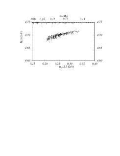
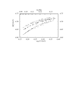
($a$)                                         
($b$)                                         

Figure 1: Result for the allowed region in the $M_{b}^{1S}$-$\alpha_{s}$ plane for the unconstrained fit based on the theoretical moments at NNLO (a) and NLO (b). The dots represent points of minimal $\chi^{2}$ for a large number of random choices within the ranges (20) and the sets (21). Experimental errors are not displayed. The two-loop running has been employed for the strong coupling.

The result for the allowed region for $M_{b}^{1S}$ and $\alpha_{s}(M_{Z})$ for the unconstrained fit using the full NNLO expressions for the theoretical moments is displayed in Fig. 1a. To illustrate the improvement coming from the NNLO corrections we have also displayed the result for the NLO theoretical moments in Fig. 1b. The dots represent the points of minimal $\chi^{2}$ for a large number of random choices within the ranges (20) and the sets (21). Comparing to the corresponding results in the pole mass scheme (see Fig. 10 and 12 in Ref. [4]) we find that the range of the mass values covered by the dots is smaller in the $1S$ scheme. For the NNLO moments the covered range for the $1S$ mass is $4.67~{}\mbox{GeV}<M_{b}^{1S}<4.72$ GeV (versus $4.76~{}\mbox{GeV}<M_{b}^{pole}<4.85$ GeV in the pole scheme [4]). However, the range of $\alpha_{s}$ covered in the $1S$ scheme is as large (slightly larger) as in the pole scheme at NNLO (NLO). This is not unexpected because of the reduced correlation of the theoretical moments to the strong coupling mentioned before. Obviously, the strong coupling determined from the $\Upsilon$ sum rules in the $1S$ scheme contains uncertainties which are much larger than the current world averages. We conclude that the $\Upsilon$ sum rules are not very competitive tool to determine the strong coupling. We therefore abandon the unconstrained fit also for the mass determination and turn to the constrained fit.

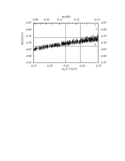
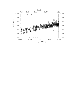
($a$)                                         
($b$)                                         

Figure 2: Result for the allowed $M_{b}^{1S}$ values for a given value of $\alpha_{s}$ at NNLO (a) and NLO (b). The dots represent points of minimal $\chi^{2}$ for a large number of random choices within the ranges (20) and the sets (21), and randomly chosen values for the strong coupling $\alpha_{s}(2.5~{}\mbox{GeV})$. Experimental errors at the $95\%$ CL level are displayed as vertical lines. It is illustrated how the allowed range for $M_{b}^{1S}$ is obtained if $0.114\leq\alpha_{s}(M_{z})\leq 0.122$ is taken as an input. The two-loop running has been employed for the strong coupling.

In Fig. 2a the allowed range for $M_{b}^{1S}$ is displayed as a function of $\alpha_{s}$ based on the NNLO theoretical moments. Fig. 2b shows the result of the same analysis using the NLO theoretical moments only. Each dot represents the $1S$ mass for which the $\chi^{2}$ function is minimal for a given input value of $\alpha_{s}$, and for a random choice within the ranges (20) and the sets (21). The statistical errors corresponding to $95\%$ CL are below $15$ MeV for all the dots displayed in Figs. 2a and b. In contrast to the constrained fit results in the pole scheme (see Fig. 13 in Ref. [4]) we find that in the $1S$ scheme the correlation between the mass and the strong coupling is reduced considerably. Compared to the pole mass results the uncertainties are smaller by a factor three for the NLO as well as the NNLO analyses. Comparing Fig. 2a and b we also see that the NNLO contributions to the moments reduce the uncertainties of the NLO analysis roughly by a factor two. Taking $\alpha_{s}(M_{z})=0.118\pm 0.004$ as input we arrive at

$$M_{b}^{1S}\,=\,4.71\pm 0.03~{}\mbox{GeV}$$ (22)

for the $1S$ mass obtained from the NNLO theoretical moments, where also the experimental errors have been taken into account. This result is consistent with the unconstrained fit shown in Fig. 1a. The NLO analysis yields $M_{b}^{1S}\,=\,4.70\pm 0.06$ GeV. Due to the small correlation of the $1S$ mass to the strong coupling the result does not change significantly if a slightly different choice of the central value and the error of $\alpha_{s}(M_{Z})$ is assumed. Eq. (22) represents the main result of this paper. We note that the choice of the range of the renormalization scale $\mu_{\rm soft}$ has the main impact on the uncertainty in the $1S$ mass determination. We have checked that allowing for larger values of $\mu_{\rm soft}$ does not affect the results displayed in Figs. 2. However, the uncertainties are larger if values of $\mu_{\rm soft}$ smaller than $1.5$ GeV are admitted. If a lower bound for $\mu_{\rm soft}$ of $1$ GeV is chosen, the result for the $1S$ mass reads $M_{b}^{1S}=4.73\pm 0.05$ GeV using the NNLO theoretical moments. However, we believe that $\mu_{\rm soft}\geq 1.5$ GeV is already a conservative choice.

To conclude this section we would like to note that our method to extract the $1S$ bottom quark mass based on the $\chi^{2}$ function for several moments (see Eq.(19)) leads to smaller uncertainties than if the fit would be carried out for individual moments independently. This can be easily seen if the scale dependence of the moments shown in Tab. 3 is compared to their mass dependence shown in Tab. 2. The $\chi^{2}$ function has a smaller scale dependence than the individual moments because it puts higher weight on linear combinations of the moments which are more sensitive to the relative size than to the absolute size of the moments. These linear combinations are determined from the entries of the covariance matrix (see Eqs. (81) and (82) of Ref. [4]) which account for the correlation of the experimental moments in Eq. (13) coming from their dependence on the $\Upsilon$ masses and electronic widths.

5 Determination of the $\overline{\mbox{MS}}$ Mass and the Upsilon Expansion

The $1S$ mass is, by construction, optimally adapted to reduce the dependence of the theoretical moments on the strong coupling and the renormalization scale $\mu_{\rm soft}$, which govern the non-relativistic dynamics of the bottom-antibottom quark pair. By the same token, the $1S$ mass does not know much about large momenta above the inverse Bohr radius $\sim M_{b}\,\alpha_{s}$. Thus, although the $1S$ mass can, like the $\overline{\mbox{MS}}$ mass, serve as a proper short-distance mass definition in its own right, it can only serve as a specialised short-distance mass definition for systems where the characteristic momentum scale is comparable to the inverse Bohr radius. For high energy processes, where momenta of order $M_{b}$ and higher are the characteristic scales, the $\overline{\mbox{MS}}$ mass is much better adapted. Thus, it is mandatory to determine the $\overline{\mbox{MS}}$ mass from the value of the $1S$ mass given in Eq. (22). We emphasise again that using specialised short-distance masses can reduce perturbative uncertainties because correlations are minimised. This is a consequence of the fact that usually only a few low orders of perturbation theory are known.

Great care has to be taken if the $\overline{\mbox{MS}}$ mass is expressed in terms of the $1S$ mass in order to ensure the proper cancellation of the most IR sensitive terms which exist in the perturbative series which expresses both masses in terms of $M_{b}^{pole}$. It has been shown in Ref. [11, 12] that the consistent way to relate the $1S$ and the $\overline{\mbox{MS}}$ mass to each other is the upsilon expansion. The upsilon expansion states that the LO, NLO and NNLO non-relativistic contributions in Eq. (1) are of order $\epsilon$, $\epsilon^{2}$ and $\epsilon^{3}$, respectively, of the auxiliary parameter $\epsilon=1$ mentioned already in Sec. 2. On the other hand, in the relation which expresses the pole mass in terms of the $\overline{\mbox{MS}}$ mass the terms of order $\epsilon$, $\epsilon^{2}$ and $\epsilon^{3}$ in the upsilon expansion correspond to the one-, two- and three-loop contributions, respectively. When the $\overline{\mbox{MS}}$ mass is expressed in terms of the $1S$ mass we then have to use the expansion in $\epsilon$ instead of $\alpha_{s}$. This means that at each order in $\epsilon$ different orders of $\alpha_{s}$ are mixed together. This unusual prescription can be understood from the fact that the most IR sensitive contributions in Eq. (1) (i.e. those contributions which involve the highest power of $\beta_{0}$ in each order) involve powers of the logarithmic term $L=\ln(\mu/C_{F}\,a_{s}\,M_{b}^{pole})$. These logarithmic terms exponentiate at larger orders, $\sum_{i=0}L^{i}/i!\approx\exp(L)=\mu/C_{F}\,a_{s}\,M_{b}^{pole}$, and effectively cancel one power of $\alpha_{s}$ [11, 12]. We will show below that this exponentiation is already very effective at NNLO in Eq. (1) making the use the upsilon expansion mandatory to achieve a reliable determination of the $\overline{\mbox{MS}}$ mass.

The upsilon expansion states that we need the three-loop contribution in the relation between the $\overline{\mbox{MS}}$ and the pole mass in order to be able to make use of the known NNLO contribution $\Delta^{NNLO}$ in Eq. (1). For the purpose of illustration we will use in the following the large-$\beta_{0}$ approximation for the yet unknown three-loop contributions. The relation between the pole and the $\overline{\mbox{MS}}$ mass then reads [23, 24]

$$M_{b}^{pole} = \overline{m}_{b}(\overline{m}_{b})\,\bigg{[}\,1+0.424\,\alpha_{s}(\overline{m}_{b})\,\epsilon+0.158\,\alpha_{s}^{2}(\overline{m}_{b})\,(\beta_{0}-2.384)\,\epsilon^{2}+0.047\,\alpha_{s}^{3}(\overline{m}_{b})\beta_{0}^{2}\,\epsilon^{3}\,\bigg{]}\,.$$ (23)

Combining Eq. (1) with Eq. (23) using the upsilon expansion up to $\epsilon^{3}$ we arrive at the following result for the $\overline{\mbox{MS}}$ bottom quark mass

$$\overline{m}_{b}(\overline{m}_{b}) = \bigg{[}\,4.71\,-\,0.40\,\epsilon\,-\,0.11\,\epsilon^{2}\,-\,0.04\,\epsilon^{3}\,\pm\,0.03\,\Big{(}\delta M_{b}^{1S}\Big{)}\,\pm\,x\,0.01\,\Big{(}\delta\alpha_{s}\Big{)}\,\bigg{]}\,\mbox{GeV}$$ (24)

where we have taken Eq. (22) as input for the $1S$ mass and assumed $\alpha_{s}(M_{z})=0.118\pm x\,0.001$ for the strong coupling. If the actual three-loop contribution in Eq. (23) is just $10\%$ smaller than the large-$\beta_{0}$ approximation, the $\epsilon^{3}$ term in Eq. (24) is smaller by a factor of two. This illustrates the effectiveness of the exponentiation of the logarithmic terms mentioned above already at NNLO in Eq. (1). We emphasise that, because of this large cancellation, the $\overline{\mbox{MS}}$ mass would have a large (positive) systematic error if the NNLO contribution in Eq. (1) would be used without also including the three-loop contributions in Eq. (23). This systematic shift would amount to about $+200$ MeV. Thus at present stage we have to leave out all $\epsilon^{3}$ terms completely, and, assuming an uncertainty in $\alpha_{s}(M_{Z})$ of $0.004$ ($x=4$), we arrive at

$$\overline{m}_{b}(\overline{m}_{b}) = 4.20\,\pm\,0.06~{}\mbox{GeV}$$ (25)

for the $\overline{\mbox{MS}}$ bottom quark mass. To obtain the error in Eq. (25) we have added all errors quadratically assuming a perturbative uncertainty due to ignorance of the exact size of the $\epsilon^{3}$ terms of $40$ MeV. We believe that our optimistic assumption about the perturbative uncertainty is justified in view of the good quality of the large-$\beta_{0}$ approximation which can be expected at the three-loop level in Eq. (23). In order to reduce the uncertainty in the $\overline{\mbox{MS}}$ bottom quark mass the three-loop contributions in the relation between the $\overline{\mbox{MS}}$ and the pole mass must be determined and the precision of the strong coupling has to be improved.

6 The Low Scale Running and the Potential Subtracted Bottom Quark Masses

In recent literature there have been two other proposals for specialised short-distance mass definitions which can be used for a stable and correlation-reduced bottom quark mass determination from the $\Upsilon$ sum rules.

In Refs. [25, 22] the “low scale running mass”, $M_{b}^{LS}$, was proposed to subtract the low momentum behaviour of the bottom quark self energy in the pole mass scheme. Like the $1S$ mass the “low scale running mass” was originally devised to improve the convergence of the perturbative contributions in inclusive $B$ meson decays. Apart from the renormalization scale which governs the strong coupling the low scale running mass depends, in addition, on the cutoff $\mu_{LS}$ which limits the momenta subtracted from the self energy. If this cutoff is adjusted to be close to the inverse Bohr radius the low scale running mass acts very similar as the $1S$ mass. The relation between $M_{b}^{LS}$ and the pole mass is known to two-loop order [26], which corresponds to order $\epsilon^{2}$ in the upsilon expansion. In order to allow for compatibility checks for sum rule analyses and other bottom quark mass determinations within the framework of the low scale running mass scheme, it is useful to determine $M_{b}^{LS}$ from the $1S$ mass obtained in this work. Taking the large-$\beta_{0}$ approximation for the yet unknown three-loop (order $\epsilon^{3}$ in the upsilon expansion) contribution, following Ref. [5], and using again the upsilon expansion one can determine $M_{b}^{LS}(\mu_{LS})$ from our result for the $1S$ mass in Eq. (22). For $\mu_{LS}=1$ GeV the result reads

$$M_{b}^{LS}(\mu_{LS}=1~{}\mbox{GeV}) = \bigg{[}\,4.71\,-\,0.09\,\epsilon\,-\,0.05\,\epsilon^{2}\,-\,0.02\,\epsilon^{3}\,$$ (26)

$$\mbox{\hskip 28.45274pt}\pm\,0.03\,\Big{(}\delta M_{b}^{1S}\Big{)}\,\pm\,x\,0.003\,\Big{(}\delta\alpha_{s}\Big{)}\,\pm\,0.01\,\Big{(}\mu\Big{)}\,\bigg{]}~{}\mbox{GeV}\,,$$

assuming again $\alpha_{s}(M_{Z})=0.118\pm x\,0.001$ for the strong coupling as input and choosing $\mu=5$ GeV as the renormalization scale of the strong coupling. The third uncertainty in Eq. (26) arises from the variation of this renormalization scale of the strong coupling between $2.5$ and $10$ GeV. In the relation between the $1S$ and the low scale running mass it is reasonable to choose the renormalization scale of order the bottom quark mass because the physical effects involving the inverse Bohr radius are eliminated. [Allowing for $\mu=1.5$ GeV would not change the result shown in Eq. (26).] The uncertainty from $\alpha_{s}$ in Eq. (26) (and also in Eq. (28)) is smaller than in the corresponding uncertainty in Eq. (24) because the order $\epsilon$ term is much smaller in Eq. (26) (and in Eq. (28)). The relation between $M_{b}^{LS}$ and $M_{b}^{1S}$ is very well behaved illustrating the fact the both are short-distance masses. The size of the scale uncertainty is compatible with the size of the $\epsilon^{3}$ term. Assuming an uncertainty of $0.004$ ($x=4$) for $\alpha_{s}(M_{Z})$ and taking into account that the exact $\epsilon^{3}$ contribution is not yet known we arrive at

$$M_{b}^{LS}(\mu_{LS}=1~{}\mbox{GeV}) = 4.57\pm 0.04~{}\mbox{GeV}$$ (27)

for the low scale running mass at $1$ GeV. As in the previous section we have combined the error coming from $M_{b}^{1S}$, $\alpha_{s}$, and a perturbative uncertainty of $20$ MeV quadratically. The result for the low scale running mass in Eq. (27) is compatible with a recent determination of $M_{b}^{LS}(\mu_{LS}=1~{}\mbox{GeV})$ which was also based on the $\Upsilon$ sum rules at NNLO ($M_{b}^{LS}=4.56\pm 0.06$ GeV) [5]. The analysis of Ref. [5], however, is different from ours with respect to several aspects. In Ref. [5] the energy denominators in the cross section $R(s)$ have been resummed for energies close to the resonances, and the final dispersion integration (11) has been carried out numerically, which means that the moments calculated in Ref. [5] contain certain non-relativistic contributions beyond NNLO. In this work the energy denominators are not resummed and all integrations are carried out analytically, consistently dropping all higher order non-relativistic contributions beyond NNLO (see Ref. [4] for details). This means that our analysis only uses global duality arguments, whereas Ref. [5] also relies on the validity of local duality. In addition, in Ref. [5] larger values of $n$ ($n=14-18$) and larger values of the soft scale $\mu_{\rm soft}$ ($\mu_{\rm soft}=2-4.5$ GeV) where used, and $M_{b}^{LS}$ was determined from extracting values for the pole mass first and converting them into numbers for the low scale running mass afterwards. In our analysis the pole mass has been eliminated completely. We also point out that in Ref. [5] the values of $M_{b}^{LS}$ were obtained by fitting individual moments whereas in this work a $\chi^{2}$ function based on several moments was employed (see the comment at the end of Sec. 4). The compatibility of Eq. (27) with the result obtained in Ref. [5] might serve as an argument that the methodical differences in this analysis and the one in Ref. [5] do not affect the mass determination.

In Ref. [10] the “potential subtracted”,$M_{b}^{PS}$, mass was proposed. It subtracts the low momentum contribution of the static potential in the pole mass scheme [15, 16, 17]. Like the low scale running mass the potential subtracted mass depends on a cutoff, $\mu_{PS}$. For $\mu_{PS}=\frac{4}{3}\mu_{LS}$ the low scale running and the potential subtracted mass are approximately equal. This equivalence is based on the universality of the most infrared sensitive contributions contained in the corresponding subtractions. So far there has not been any sum rule analysis which has attempted to extract the potential subtracted bottom quark mass. However, it is useful to determine $M_{b}^{PS}$ from the $1S$ mass value obtained in this work to allow for cross checks with possible future work on this subject. Because the potential subtracted mass is based on the static perturbative potential, which is known to NNLO in the non-relativistic expansion (i.e. $\epsilon^{3}$ in the upsilon expansion), the perturbative uncertainties in the relation between potential subtracted and $1S$ mass are smaller. Starting from our result for the $1S$ mass, Eq. (22), the potential subtracted mass at the subtraction scale $\mu_{PS}=2$ GeV reads

$$M_{b}^{PS}(\mu_{PS}=2~{}\mbox{GeV}) = \bigg{[}\,4.71\,-\,0.13\,\epsilon\,-\,0.04\,\epsilon^{2}\,-\,0.01\,\epsilon^{3}\,$$ (28)

$$\mbox{\hskip 28.45274pt}\pm\,0.03\,\Big{(}\delta M_{b}^{1S}\Big{)}\,\pm\,x\,0.003\,\Big{(}\delta\alpha_{s}\Big{)}\,\pm\,0.01\,\Big{(}\mu\Big{)}\,\bigg{]}~{}\mbox{GeV}\,,$$

where we have again assumed $\alpha_{s}(M_{Z})=0.118\pm x\,0.001$ as an input for the strong coupling. The third uncertainty arises from the variation of the renormalization scale in the strong coupling between $2.5$ and $10$ GeV. The relation between $M_{b}^{PS}$ and $M_{b}^{1S}$ is very well behaved illustrating the fact that $M_{b}^{PS}$ is also a short-distance mass. Assuming again an uncertainty of $0.004$ ($x=4$) for $\alpha_{s}(M_{Z})$, taking a perturbative uncertainty of $10$ MeV and adding all errors quadratically we arrive at

$$M_{b}^{PS}(\mu_{PS}=2~{}\mbox{GeV}) = 4.53\pm 0.03~{}\mbox{GeV}$$ (29)

for the potential subtracted mass at $2$ GeV.

To conclude this section we note that it is possible to tune the cutoff scales in the low scale running and the potential subtracted masses, at each order of perturbation theory, such that the correlations of the mass to other parameters are minimal. Such a fine-tuning approach, however, is illegal because from the conceptual point of view any cutoff scale close to the inverse Bohr radius is equally well suited. This “scale-ambiguity” is a specific characteristic of the low scale running and the potential subtracted mass and not inherent in the $1S$ mass, because the latter is defined through a bound state mass, which is a physical quantity. We therefore consider the $1S$ scheme as the most natural mass scheme to be used to describe processes involving heavy quark-antiquark pairs in the non-relativistic regime. We emphasise, however, that the $LS$, $PS$ and $1S$ mass improve the quality of the mass extraction from the $\Upsilon$ sum rules all by the same mechanism, and that the most infrared sensitive contributions contained in the subtractions are equivalent in all schemes. In the $1S$ scheme the cutoff which is visible in the definition of the $LS$ and the $PS$ masses is provided in a natural way by the width of the wave-function of the ${}^{3}\!S_{1}$ bottom-antibottom quark bound state. No matter which scheme is used the final answers for the $\overline{\mbox{MS}}$ bottom quark mass should be compatible.

7 Conclusions

In this work we have extracted the $1S$ mass, $M_{b}^{1S}$, from sum rules which relate the masses and electronic decay widths of the $\Upsilon$ mesons to large-$n$ moments of the vacuum polarization function, which have been calculated at NNLO in the non-relativistic expansion. $M_{b}^{1S}$ is defined as half the perturbative mass of a $J^{PC}=1^{--}$, ${}^{3}\!S_{1}$ bottom-antibottom quark bound state, i.e. it represents the perturbative contribution of half the mass of the $\Upsilon(1S)$ meson. However, the latter information is not used in this work and $M_{b}^{1S}$ is considered as a fictitious mass parameter which is determined solely from the sum rule analysis. The result for the $1S$ mass reads $M_{b}^{1S}=4.71\pm 0.03$ GeV, if $\alpha_{s}(M_{Z})=0.118\pm 0.004$ is taken as an input for the strong coupling, and has only a small correlation to the choice of $\alpha_{s}$. The close proximity of this result to $M_{\Upsilon(1S)}/2$ is non-trivial because higher excitations and the $b\bar{b}$ continuum have a non-negligible contribution to the sum rules for the values of $n$ used in this work. The fact that, within the errors, $M_{b}^{1S}$ is equal to $M_{\Upsilon(1S)}/2=4.730$ GeV indicates that the non-perturbative contributions in the ${\Upsilon(1S)}$ mass are probably small. Compared to an earlier work which has been carried out in the pole mass scheme by the same author we find an improved perturbative behaviour of the moments and a much smaller residual dependence on the renormalization scale which governs the non-relativistic dynamics of the bottom-antibottom quark pair. The $1S$ bottom quark mass is a short-distance mass (i.e. it does not have an ambiguity of order $\Lambda_{QCD}$) and can be used as a mass parameter in its own right. It is well adapted to processes where the characteristic scale is below the bottom quark mass and has been successfully applied earlier to inclusive $B$ mesons decays, where it leads to a significant improvement in the behaviour of the perturbative series describing the inclusive widths. [11, 12]

Because $M_{b}^{1S}$ is a short-distance mass it has a well behaved perturbative relation to the $\overline{\mbox{MS}}$ mass, which is adapted to processes where the characteristic scale is of order the bottom quark mass or higher. In order to relate the $1S$ mass to the $\overline{\mbox{MS}}$ mass definition it is mandatory to use the upsilon expansion [11, 12] in order to ensure the cancellation of large infrared-sensitive contributions present in the perturbative series which relate both masses to the pole mass. Using the presently known two-loop contributions in the relation of the $\overline{\mbox{MS}}$ and the pole mass (i.e. using the upsilon expansion up to order $\epsilon^{2}$) and assuming $\alpha_{s}(M_{Z})=0.118\pm 0.004$ we arrive at $\overline{m}_{b}(\overline{m}_{b})=4.20\pm 0.06$ GeV for the $\overline{\mbox{MS}}$ mass. The error in the $\overline{m}_{b}(\overline{m}_{b})$ can be reduced once the three-loop contributions in the relation between the $\overline{\mbox{MS}}$ and the pole mass are calculated and if the precision in $\alpha_{s}$ is increased.

References

- [1] M. B. Voloshin, Int. J. Mod. Phys. A 10 (1995) 2865.
- [2] J. H. Kühn, A. A. Penin, and A. A. Pivovarov, Nucl. Phys. B 534 (1998) 356.
- [3] A. A. Penin, and A. A. Pivovarov, Phys. Lett. B 435 (1998) 413.
- [4] A. H. Hoang, Phys. Rev. D 59 (1999) 014039 [hep-ph/9803454]
- [5] K. Melnikov and A. Yelkhovkii, Phys. Rev. D 59 (1999) 114009
- [6] M. Jamin and A. Pich, Nucl. Phys. B 507 (1997) 334.
- [7] M. Beneke and V. M. Braun, Nucl. Phys. B 426 (1994) 301.
- [8] I. I. Bigi et al., Phys. Rev. D 50 (1994) 2234.
- [9] A. H. Hoang, M. C. Smith, T. Stelzer and S. S. Willenbrock, Phys. Rev. D 59 (1999) 114014 [hep-ph/9804227]
- [10] M. Beneke, Phys. Lett. B 434 (1998) 115.
- [11] A. H. Hoang, Z. Ligeti and A. V. Manohar, Phys. Rev. Lett. 82 (1999) 277.
- [12] A. H. Hoang, Z. Ligeti and A. V. Manohar, Phys. Rev. D 59 (1999) 074017 [hep-ph/9811239].
- [13] Particle Data Group, C. Caso et al, Eur. Phys. J. C 3 (1998) 1.
- [14] A. Pineda and F. J. Yndurain, Phys. Rev. D 58 (1998) 094022.
- [15] W. Fischler, Nucl. Phys. B 129 (1977) 157.
- [16] A. Billoire, Phys. Lett. B 92 (1980) 343.
- [17] Y. Schröder, Phys. Lett. B 447 (1999) 321.
- [18] M. Peter, Phys. Rev. Lett. 78 (1997) 602; Nucl. Phys. B 501 (1997) 471.
- [19] H. Albrecht et al., Z. Phys. C 65 (1995) 619.
- [20] E. C. Poggio, H. R. Quinn, and S. Weinberg, Phys. Rev. D 13 (1976) 1958.
- [21] W. E. Caswell and G. E. Lepage, Phys. Lett. B 167 (1986) 437.
- [22] I. Bigi, M. Shifman, N. Uraltsev and A. Vainshtein, Phys. Rev. D 56 (1997) 4017.
- [23] N. Gray et al., Z. Phys. C 48 (1990) 673.
- [24] P. Ball, M. Beneke and V.M. Braun, Nucl. Phys. B 452 (1995) 563.
- [25] M. B. Voloshin, Phys. Rev. D 46 (1992) 3062.
- [26] A. Czarnecki, K. Melnikov and N. Uraltsev, Phys. Rev. Lett. 80 (1998) 3189.