Monopoles and Coulomb Gas Representation of the QCD Effective Lagrangian

Abstract

A novel Coulomb gas (CG) description of low energy $QCD_{4}(N_{c})$ is constructed. The construction is based on the dual transformation of the $QCD$ effective Lagrangian. By considering a large gauge transformation, the charges of this statistical system are identified with magnetic monopoles which carry fractional charges of strength $1/N_{c}$. Furthermore, the creation operator which inserts the magnetic charge in the CG picture is explicitly constructed and demonstrated to have a non-zero vacuum expectation value, indicating that confinement does occur. The Wilson loop operator as well as the creation operator for the domain wall in CG representation is also constructed. Additional support for the D-brane picture suggested by Witten is also found. Lastly, the relation of the CG picture with the instanton-quarks is also discussed.

PACS codes:

I Introduction

Color confinement, spontaneous breaking of chiral symmetry, the $U(1)$ problem, $\theta$ dependence, and the classification of vacuum states are some of the most interesting questions in $QCD$. Unfortunately, the progress in our understanding of them is extremely slow. At the end of the 1970s A. M. Polyakov [1] demonstrated color confinement in $QED_{3}$; this was the first example in which nontrivial dynamics was a key ingredient in the solution. Soon after, ’t Hooft and Mandelstam [2] suggested a qualitative picture of how confinement could occur in $QCD_{4}$. The key point, the ’t Hooft - Mandelstam approach, is the assumption that dynamical monopoles exist and Bose condense. Many papers have been written on this subject since the original formulation [2]; however, the main questions, such as, “What are these monopoles?”; “How do they appear in the gauge theories without Higgs fields?”; “How do they interact?”, were still not understood (for a recent review see [3]). Almost 20 years passed before the next important piece of the puzzle was solved [4]. Seiberg and Witten demonstrated that confinement occurs in SUSY $QCD_{4}$ due to the condensation of monopoles much along the lines suggested many years ago by ’t Hooft and Mandelstam. Furthermore, condensation of dyons together with oblique confinement for nonzero vacuum angle, $\theta$, was also discovered in SUSY models (a phenomenon which was also argued to take place in ordinary $QCD$; see [3]). In addition to forming concrete realizations of earlier ideas, the recent progress in SUSY models has introduced many new phenomena, such as the existence of domain walls[5] which connect two distinct $\theta$-vacua. New insights into confinement was also recently given by Witten [6], in which he argued that domain walls connecting two vacua labeled by $k$ and $k+1$ behave similarly to $D$-branes on which the $SQCD$ strings can end. It is tantalizing to suggest that such phenomenon also take place in $QCD$; indeed, in this paper it is argued that this in fact does occur.

With such a wealth of information now available for SUSY gauge theories, it is interesting to ask how one can apply that knowledge to QCD. In a recent review Shifman [5] addressed certain aspects of this question and we refer to that paper for further references and recent development. Thus far, most works have approached such questions by starting with a supersymmetric theory where some particular dynamical aspect of interest is already known; then introducing explicit supersymmetry breaking terms by giving the gluinos or squarks mass; finally, in the limit of infinite mass one recovers a non-supersymmetric theory with decoupled gluinos and squarks. Unfortunately, any calculations in this limit are beyond reach. Consequently, theories with a small SUSY breaking mass term are usually studied and a qualitative picture of what happens in QCD (and other non-supersymmetric theories) is extracted. This procedure has lead to success in the identification of the complicated vacuum structure for such theories: there are $N$ inequivalent vacua for each given $\theta$ [5]. These vacua are distinguished by the phase of the chiral condensate and there are domain walls which interpolate between them. It is believed that in QCD such a similar structure exists.

Rather than beginning with the SUSY model and then breaking the symmetry, our analysis begins with non-supersymmetric $QCD$. For the purposes of the paper it will be assumed that the theory is in the confining phase and that chiral symmetry is broken. The question to be addressed is then: “Does the picture which emerges in SUSY models reflect what happens in QCD?”. We will demonstrate that the answer is indeed yes. This strategy clearly does not prove confinement, nor does it elaborate on the microscopic mechanism responsible for it, however, it will, however, demonstrate that the assumption of confinement implies the condensation of massless monopoles and vice versa. Furthermore, the role that the $\theta$ parameter plays in the condensation of dyons with non-zero electric charge will be illuminated. In addition, this strategy will allow us to demonstrate that the states in QCD for each given $\theta$-angle is indeed classified by the integer number $k$ labeling the phase of the dyon condensate. Finally, domain walls which interpolate between these different phases will be shown to have wall tension $\sim{N}$, and it is consistent with their interpretation as $D$-branes rather than as QCD string solitons. In addition, a relationship between the dual representation of low energy QCD, in terms of the Coulomb Gas of monopoles, and instantons will be discussed. This leads us to conjecture that at large distances our particles with fractional magnetic charges, from the CG representation, are in fact the instanton-quarks suspected long ago [7].

Before going into a detailed analysis of the effect Lagrangian the starting point of our analysis will now be elaborated on. Experience in SUSY models demonstrates that the effective Lagrangian approach and duality transformations are very effective tools in the analysis of the large distance dynamics in the strong coupling regime (see e.g. reviews [8]). These tools will be adopted for the study of QCD. The first key element in the analysis is the effective Lagrangian approach. As is well known, there are two different definitions of an effective Lagrangian in quantum field theory. One of them is the Wilsonian effective Lagrangian describing the low energy dynamics of the lightest particles in the theory. In QCD, this is implemented by effective chiral Lagrangians for the pseudoscalar mesons. Another type of the effective Lagrangian (potential) is defined as the Legendre transform of the generating functional for connected Greens functions. This object is useful in addressing questions about the vacuum properties of the theory in terms of vacuum expectation values (VEV’s) of composite operators, as they minimize the effective action. Such an approach is well suited for studying the dependence of the vacuum state on external parameters, such as the light quark masses or the vacuum angle $\theta$. However, it is not useful for studying, for instance, $S$-matrix elements because the kinetic term cannot be recovered in such an approach. The utility of such an approach to gauge theories has been recognized long ago for supersymmetric models, where the anomalous effective potential has been found for both the pure gauge case [9] and $SQCD$ [10]. Properties of the vacuum structure in SUSY models were correctly understood only after analyzing this kind of effective potential. The second key point of our approach is the observation that such an effective potential in QCD (which is a collection of self-interacting Sine-Gordon (SG) fields) has a dual representation in terms of a Coulomb Gas of several species of charges, which will be described in detail in Section 3.

Since our description starts from color-singlet fields (the phases of the chiral condensate), one might think that no information about confinement, which is clearly a color phenomena, can be extracted from such an analysis. However, contrary to ones instinct, it is possible to obtain color information due to the existence of the free parameter $\theta$, which plays the role of the messenger between colorless and colorful objects. Indeed, the dependence of the physical observables as a function of $\theta$ can be studied exclusively in terms of the colorless degrees of freedom by using the effective Lagrangian approach. Furthermore, the manner in which the theory transforms under both large gauge transformations and under the variation of the $\theta$ parameter, when monopoles (colorful object) acquire a color electric charge, are known independently. Consequently, understanding the $\theta$ dependence gives us an understanding of confinement, as $\theta$ acts as a link between colorless and colorful degrees of freedom.

This paper is an extended version of the letter [11] and is organized as follows: In Section 2 we overview the properties of the effective Lagrangian of QCD[12]. Section 3 is devoted to derivation of the Coulomb gas representation of this effective Lagrangian, this representation can be interpreted as a dual form of the original low-energy effective field theory; the massless particles of the new statistical mechanical problem are identified with monopoles; the measure for this statistical ensemble is further analyzed and it is then argued that our particles can be identified with instanton-quarks. In Section 4 several consequences of the Coulomb gas representation are derived, in particular, the expression for the monopole creation-operator (magnetization) is obtained and its VEV calculated; The magnetic potential in the presence of the domain walls is also discussed and it is argued that the QCD string can end on the domain wall.

II Effective Lagrangian and $\theta$ dependence in QCD

Our analysis begins with the effective low energy $QCD$ action derived in [12], which allows the $\theta$-dependence of the ground state to be analyzed and is crucial to the identification of monopole charges. Within this approach, the Goldstone fields are described by the unitary matrix $U_{ij}$, which correspond to the $\gamma_{5}$ phases of the chiral condensate: $\langle\overline{\Psi}_{L}^{i}\Psi_{R}^{j}\rangle=-|\langle\overline{\Psi}_{L}\Psi_{R}\rangle|\,U_{ij}$ with

$$U=\exp\left[i\sqrt{2}\,\frac{\pi^{a}\lambda^{a}}{f_{\pi}}+i\frac{2}{\sqrt{N_{f}}}\frac{\eta^{\prime}}{f_{\eta^{\prime}}}\right],\quad UU^{+}=1,$$ (1)

where $\lambda^{a}$ are the Gell-Mann matrices of $SU(N_{f})$, $\pi^{a}$ is the pseudoscalar octet, and $f_{\pi}=133\;MeV$. In terms of $U$ the low-energy effective potential is given by[12]:

$$W_{QCD}(\theta,U)=-\lim_{V\rightarrow\infty}~{}\frac{1}{V}~{}\log\sum_{l=0}^{p-1}~{}\exp\left\{VE\cos\left(-\frac{q}{p}\theta+i\frac{q}{p}\log{\rm Det}~{}U+\frac{2\pi}{p}~{}l\right)+\frac{1}{2}V\,{\rm Tr}~{}(mU+m^{+}U^{+})\right\}.$$ (2)

All dimensional parameters in this potential are expressed in terms of the $QCD$ vacuum condensates, and are well known numerically: $m={\rm diag}(m_{q}^{i}|\langle\overline{\Psi}^{i}\Psi^{i}\rangle|)$; and the constant $E$ is related to the $QCD$ gluon condensate $E=\langle b\alpha_{s}/(32\pi)G^{2}\rangle$. The only unknown parameters in this construction are the integers $p$ and $q$ which play the same role as the discrete integer numbers classifying the vacuum states in SUSY theories. These numbers are related to a discrete symmetry which is a remnant of the anomaly, and can be found only by explicit dynamical calculations. Various arguments can be put forward which support different values of $p$ and $q$, see e.g. [13, 5]; however, in what follows $p$ and $q$ will not be fixed, rather only the ratio will be constrained so that in large $N_{c}$ limit $q/p\sim 1/N_{c}$ such that the $U(1)$ problem is resolved.

It is possible to argue that equation (2) represents the anomalous effective Lagrangian realizing broken conformal and chiral symmetries of QCD. The arguments are that:
Equation (2):

1. correctly reproduces the VVW effective chiral Lagrangian [14] in the large $N_{c}$ limit
     [ For small values of $(\theta-i\log{\rm Det}\,U)<\pi/q$, the term with $l=0$ dominates the infinite volume limit. Expanding the cosine (this corresponds to the expansion in $q/p\sim 1/N_{c}$), we recover exactly the VVW effective potential [14] together with the constant term $-E=-\langle b\alpha_{s}/(32\pi)G^{2}\rangle$ required by the conformal anomaly:

   $$W_{VVW}(\theta,U,U^{+})=-E-\frac{\langle\nu^{2}\rangle_{YM}}{2}(\theta-i\log{\rm Det}\,U)^{2}-\frac{1}{2}Tr\,(mU+m^{+}U^{+})+\ldots\;.~{}~{}~{}~{}~{}~{}~{}$$ (3)

   here we used the fact that at large $N_{c}$, $E(q/p)^{2}=-\langle\nu^{2}\rangle_{YM}$ is the topological susceptibility in pure YM theory. Corrections in $1/N_{c}$ stemming from Eq.(2) constitute a new result of Ref.[12].]

2. reproduces the anomalous conformal and chiral Ward identities of QCD
    [ Let us check that the anomalous WI’s in QCD are reproduced from Eq.(2). The anomalous chiral WI’s are automatically satisfied with the substitution $\theta\rightarrow(\theta-i\log{\rm Det}\,U)$ for any $N_{c}$, in accord with [14]. Furthermore, it can be seen that the anomalous conformal WI’s of [15] for zero momentum correlation functions of the operator $G^{2}$ in the chiral limit $m_{q}\rightarrow 0$ are also satisfied when $E$ is chosen as above. As another important example of WI’s, the topological susceptibility in QCD near the chiral limit will be calculated from Eq.(2). For simplicity, the limit of $SU(N_{f})$ isospin symmetry with $N_{f}$ light quarks, $m_{q}\ll\Lambda_{QCD}$ will be considered. For the vacuum energy for small $\theta<\pi/q$ one obtains[12]

   $$E_{vac}(\theta)=-E+m_{q}\langle\bar{\Psi}\Psi\rangle N_{f}\cos\left(\frac{\theta}{N_{f}}\right)+O(m_{q}^{2})\;.$$ (4)

   Differentiating this expression twice with respect to $\theta$ reproduces the result of [16]:

   $$\lim_{q\rightarrow 0}\;i\int dx\,e^{iqx}\langle 0|T\left\{\frac{\alpha_{s}}{8\pi}G\tilde{G}(x)\,\frac{\alpha_{s}}{8\pi}G\tilde{G}(0)\right\}|0\rangle=-\frac{\partial^{2}E_{vac}(\theta)}{\partial\,\theta^{2}}=\frac{1}{N_{f}}m_{q}\langle\bar{\Psi}\Psi\rangle+O(m_{q}^{2})\;.$$ (5)

   Other known anomalous WI’s of QCD can be reproduced from Eq.(2) in a similar fashion. Consequently, Eq.(2) reproduces the anomalous conformal and chiral Ward identities of QCD and gives the correct $\theta$ dependence for small values of $\theta$, and in this sense passes the test for it to be the effective anomalous potential for QCD. ]

3. reproduces the known results for the $\theta$ dependence at small $\theta$[14], but may lead to a different behavior for large values $\theta>\pi/q$ if $q\neq 1$
     [ As mentioned earlier, at small $\theta\ll\pi/q$ our results are identical to those found in [14]; the main difference with [14] arises when $\theta-i\log{\rm Det}\,U\sim 1$ where cusp singularities occur. These singularities are analogous to the ones arising in SUSY models and show the non-analyticity of the $\theta$ dependence at certain values of $\theta$. The origin of this non-analyticity is clear, it appears when the topological charge quantization is imposed explicitly at the effective Lagrangian level. Thus, the cusp structure of the effective potential seems to be an unavoidable consequence of the topological charge quantization (which was not explicitly imposed in the approach of [14]). ]

An interesting note is that in general the $\theta$ dependence appears in the combination $\theta/N_{c}$ which naively does not provide the desired $2\pi$ periodicity for the physical observables; however, such a behaviour is derived from Eq.(2) which does have $2\pi$ periodicity. This seeming contradiction is resolved by noting that in the thermodynamic limit, $V\rightarrow\infty$, only the term of lowest energy in the summation over $l$ is retained for a particular value of $\theta$, creating the illusion of $\theta/N_{c}$ periodicity in observables. Of course, the values $\theta$ and $\theta+2\pi$ are physically equivalent for the entire set of states, but not for a selected individual vacuum state. Consequently, the $\theta$ dependence in the infinite volume limit appearing in the combination $\theta/N_{c}$ is a result of being stuck in a particular state. The reader is referred to the original papers [12] for more detailed discussions of the properties of the effective potential (2). One final point to be made before moving on is that in general $E_{vac}(\theta)$ is a multi-valued function with cusp singularities at $\theta=\frac{(2k+1)\pi}{q}$ where one solution switches to another. Furthermore, the number of additional meta-stable vacuum states is very sensitive to the integer parameters $p$ and $q$ introduced earlier. In particular, for the physical values of the quark masses, there are $q-1$ additional local minima of the effective chiral potential, which are separated by large barriers of strength $\sim E$ from the true physical vacuum of lowest energy, but which are almost degenerate in energy, $\Delta E\sim m$. Such availability of almost degenerate vacua imply the appearance of QCD domain walls and was studied in [17]. The appearance of these walls have interesting consequences in this work as well.

This section is closed with a few technical but important remarks: The effective low energy Lagrangian described above has a very special SG structure. The fact that such a structure appears in the second term of Eq. (2), $m(U+U^{+})\sim\sum_{i}m_{i}\cos(\phi_{i})$, is quite natural and is associated with the Goldstone origin of the $\phi_{i}$ fields. The first term has a similar SG structure $\sim\cos\left(\left(\sum_{i}\phi_{i}-\theta\right)/N_{c}\right)$; however, its origin is less trivial and requires some explanation. Firstly, WI’s imply that the singlet combination $\sum_{i}\phi_{i}$ always appears with $\theta$ in the form $(\theta-i\log{\rm Det}\,U)$ [14]. Secondly, the appearance of the cosine interaction, $\cos(\theta/N_{c})$, leads to the following scenario in pure gluodynamics ($\phi_{i}$’s are frozen): the $(2k)^{\rm th}$ derivative of the vacuum energy with respect to $\theta$, as $\theta\rightarrow 0$, is expressed solely in terms of one parameter, $\frac{1}{N_{c}}$, for arbitrary $k$:

$$\left.\frac{\partial^{2k}E_{vac}(\theta)}{\partial\,\theta^{2k}}\right|_{\theta=0}\sim\int\prod_{i=1}^{2k}d^{4}x_{i}\left\langle Q(x_{1})...Q(x_{2k})\right\rangle\sim\left(\frac{i}{N_{c}}\right)^{2k},$$ (6)

where, $Q\sim G_{\mu\nu}{\widetilde{G}}_{\mu\nu}$. This property was seen as a consequence of Veneziano’s solution of the $U(1)$ problem [18]. The reason that only one factor appears in Veneziano’s calculation is that the corresponding correlation function, $\sim\int\prod_{i=1}^{2k}d^{4}x_{i}\langle Q(x_{1})...Q(x_{2k})\rangle$, becomes saturated at large distances by the Veneziano ghosts whose contributions factorize exactly, and was subsequently interpreted as a manifestation of the $\theta/N_{c}$ dependence in gluodynamics at small $\theta$. However, at that time it was incorrectly assumed that such a dependence indicates that the periodicity in $\theta$ is proportional to $N_{c}$. Later on [13] it was argued that the behavior in Eq.(6) is a consequence of the holomorphic structure for the non-perturbative part of the QCD partition function where the non-perturbative vacuum energy depends only on a single complex combination $\tau=1/g^{2}_{0}+i\frac{\theta}{32\pi^{2}}\frac{bq}{p}$ in the same way as it was in SUSY models. The behaviour in (6) was also demonstrated by “integrating in”a very heavy fermion and integrating it out afterwards, which must leave the gluodynamics unaltered [13]. All three independent arguments support the property (6), consequently Eq. (2) will be used as the defining effective action for low energy QCD.

III Coulomb Gas Representation of Low Energy Dynamics

The effective low energy $QCD$ action (2) has a very special quality, all the interactions have a trigonometric form and are in particular cosinusodal. This is the defining character of a SG model. The presence of many fields and many cosine terms with different harmonics which interact in a highly non-trivial manner serve to slightly complicate the situation. Nevertheless, many of the special properties of the SG theory apply to this model, the admittance of a Coulomb gas (CG) representation for the partition function is no different. Although this is a four dimensional theory, and questions about renormalizability of the theory may come to mind, there are no such issues here since the effective action is a low energy one. Following the usual procedure for mapping a statistical CG model into the field theoretic SG model, the CG picture that arises from the effective low energy $QCD$ action, Eq. (2), will be derived in this section. The statistical model will be seen to contain several species of charges which appear due to the presence of several cosine interactions in the field theory model. The physical meaning of these charges will be illuminated by applying large gauge transformations on the partition function and determining the manner in which the charges transform. This will lead to the identification of one of the charge species as magnetic monopoles and of the singlet combination, $\phi$, in the SG model as the magnetic scalar potential. The remaining charges will also be argued to have magnetic properties; however, it will prove difficult to construct a precise statement about them. The statistical model will then be analyzed in subsequent sections of this paper.

A Formal Derivation

Although the mapping between a SG theory and its CG representation is well known[1], in this section several illustrative steps in its derivation will be given for completeness. The existence of many fields and cosine terms only serve to make the formulae more bulky; however, the basic strategy is the same as in the standard case. Using the effective potential in Eq. (2) the defining partition function is taken to be,

$$Z=\Bigg{\langle}\exp\Bigg{\{}-\int d^{4}x\Big{\{}E\cos\left(\frac{q}{p}\left(\phi-\theta+2\pi n\right)+2\pi k\right)+m_{1}\cos(\phi_{1})+\dots+m_{N_{f}}\cos(\phi_{N_{f}})\Big{\}}\Bigg{\}}\Bigg{\rangle}$$ (7)

Here, the matrix $U$ characterizing the phases of the chiral condensate has been placed in diagonal form, $U={\rm diag}(\phi_{1},\dots,\phi_{N_{f}})$, the combination of fields $\phi={\rm Tr}~{}U$ represents the singlet, $m_{a}=m_{q}^{a}|\langle\bar{\Psi}^{a}\Psi^{a}\rangle|$ denotes the mass of the $a$-th flavor of quark together with its condensate, $E=\langle b\alpha_{s}/(32\pi)G^{2}\rangle$ is the vacuum energy of the system, and the angled brackets represent the Gaussian weighting,

$$\langle\dots\rangle=\sum_{k=0}^{p-1}\sum_{n=-\infty}^{\infty}\int{\cal D}\phi_{a}~{}\dots~{}{\rm e}^{-g^{2}\int d^{4}x\frac{1}{2}({\vec{\nabla}}\phi_{a})^{2}}$$ (8)

where $g^{2}$ is a coupling constant $\sim f_{\pi}^{2}$ so that the fields $\phi_{a}$ are dimensionless and all distances are measured in the units of $f_{\pi}^{-1}$.

The following strategy for obtaining the CG representation from the SG model will be employed here: a series expansion in the vacuum energy and the quark masses will be carried; the cosine terms will then appear outside of the exponential and are weighted by the Gaussian weighting; introducing ${\rm Z\!\!Z}_{2}$ valued fields to represent the cosine terms allows the dynamical fields to re-appear in the exponential, however, now they appear linearly; in this form it is possible to completely integrate out the dynamical fields which leads to the final CG representation. These steps are now carried out in order. Firstly, performing a series expansion in $E$ and $m_{a}$ independently leads to the following form,

$$Z = \sum_{\{M_{0},\dots,M_{N_{f}}\}=0}^{\infty}\frac{E^{M_{0}}}{M_{0}!}\frac{m_{1}^{M_{1}}}{M_{1}!}\dots\frac{m_{N_{f}}^{M_{N_{f}}}}{M_{N_{f}}!}\Bigg{\langle}\left(\int dx^{(0)}\cos\left(\frac{q}{p}\left(~{}\phi(x^{(0)})-\theta+2\pi n\right)+2\pi k\right)\right)^{M_{0}}$$ (10)

$$\hskip 233.31259pt\times~{}\prod_{a=1}^{N_{f}}\left(\int dx^{(a)}\cos(\phi_{a}(x^{(a)}))\right)^{M_{a}}\Bigg{\rangle}$$

By introducing the ${\rm Z\!\!Z}_{2}$ valued fields $Q^{(a)}$, for $a=0,\dots,N_{f}$, to replace the cosine interactions the dynamical fields can be integrated out exactly. For $a\neq 0$ the fields are introduced via,

$$\cos(\phi_{a})=\frac{1}{2}\sum_{Q^{(a)}=\pm 1}{\rm e}^{iQ_{a}\phi_{a}}\qquad,\quad a\neq 0.$$

and the charge species $Q^{(a\neq 0)}$ will be said to be dual to the field $\phi_{a}$. The singlet case, $a=0$, contains additional parameters,

$$\cos\left(\frac{q}{p}(\phi-\theta+2\pi n)+2\pi k\right)=\frac{1}{2}\sum_{Q^{(0)}=\pm\frac{q}{p}}{\rm e}^{iQ^{(0)}((\phi-\theta+2\pi n)+2\pi\frac{p}{q}k)}.$$ (11)

and the charge species $Q^{(0)}$ will be said to be dual to the singlet combination, $\phi={\rm Tr}~{}U$. The explicit presence of the $\theta$-angle in (11) is essential in identifying the physical meaning of this charge species. Inserting both expressions into the series expansion of the partition function, Eq. (10), leads to a form in which the dynamical fields appear at most quadratic in the exponential and they can be completely integrated out,

$$Z = \sum_{\{M_{0},\dots,M_{N_{f}}\}=0}^{\infty}\frac{(E/2)^{M_{0}}}{M_{0}!}\frac{(m_{1}/2)^{M_{1}}}{M_{1}!}\dots\frac{(m_{N_{f}}/2)^{M_{N_{f}}}}{M_{N_{f}}!}\int\left(dx^{(0)}_{1}\dots dx^{(0)}_{M_{0}}\right)\dots\left(dx^{N_{f}}_{1}\dots dx^{N_{f}}_{M_{N_{f}}}\right)$$ (13)

$$\hskip 85.35826pt\times\sum_{\stackrel{{\scriptstyle\scriptstyle Q^{(0)}_{i}=\pm\frac{q}{p}}}{{\{Q^{(1)}_{i},\dots,Q^{({N_{f}})}_{i}\}=\pm 1}}}\Bigg{\langle}{\rm e}^{i\sum_{b=1}^{M_{0}}Q^{(0)}_{b}\left(\phi(x^{(0)}_{b})-\theta+2\pi n+2\pi\frac{p}{q}k\right)}\prod_{a=1}^{{N_{f}}}{\rm e}^{i\sum_{b=1}^{M_{a}}Q^{(a)}_{b}\phi_{a}(x^{(a)}_{b})}\Bigg{\rangle}$$

The functional integral is trivial to perform and one arrives at the dual CG action. The brackets can then be removed, as long as the summations over $n$ and $k$ are restored. After some rewriting the CG action is,

$$S_{CG} = i\theta Q^{(0)}_{T}-\ln\left(p\sum_{n=-\infty}^{\infty}{\rm e}^{2\pi iQ^{(0)}_{T}n}\right)+\frac{1}{2g^{2}}\sum_{a=1}^{N_{f}}\Bigg{\{}\sum_{b,c=1}^{M_{0}}Q^{(0)}_{b}~{}G(x^{(0)}_{b}-x^{(0)}_{c})~{}Q^{(0)}_{c}+2\sum_{b=1}^{M_{0}}\sum_{c=1}^{M_{a}}Q^{(0)}_{b}~{}G(x^{(0)}_{b}-x^{(a)}_{c})~{}Q^{(a)}_{c}$$ (15)

$$\hskip 184.9429pt+\sum_{b,c=1}^{M_{a}}Q^{(a)}_{b}~{}G(x^{(a)}_{b}-x^{(a)}_{c})~{}Q^{(a)}_{c}\Bigg{\}}.$$

Here, $Q^{(0)}_{T}=\sum_{b=1}^{M_{0}}Q^{(0)}_{b}$ is the total $Q^{(0)}$ charge for that configuration, $G(x-y)$ denotes the relevant Greens function of the Laplace operator ($-\Box G(x-y)=\delta(x-y)$), and the factor of $p$ appears due to the redundancy introduced by the summation over $k$ in Eq.(8).

Notice that the fugacities of the charge species $Q^{(a\neq 0)}$ are given by the masses of the $a^{\rm th}$ quark, while the fugacity of the charge species $Q^{(0)}$ is proportional to the gluon condensate $E$. An important point is that the fugacity of charge species $Q^{(a\neq 0)}$ vanishes in the chiral limit, while that of the $Q^{(0)}$ charges remains non-zero. A second point is that, in the chiral limit, this representation does not obviously have invariance in $\theta$, while in $QCD$ the $\theta$-angle appears with quark masses and hence disappears in this limit. It is possible to demonstrate that the partition function has this property; however, because its proof is rather technical, the details are deferred to appendix A.

There are several important features of the action (15) which should be noted. Firstly, the summation over $n$ forces the total $Q^{(0)}$ charge, $Q_{T}^{(0)}$, to be an integer. Such a constraint is the analog of the quantization of the topological charge and is to be expected. Additionally, since this species has charges $\sim\frac{q}{p}\sim 1/N_{c}$, this constraint enforces a fractional quantization on the total charges: the difference in the number of positive and negative charges of species $Q^{(0)}$ must be an integer multiple of $N_{c}$. Secondly, the $\theta$-angle only interacts with the $Q^{(0)}$ species. This directly results from the $Q^{(0)}$ species being dual to the singlet field $\phi$, which is the only field directly interacting with the $\theta$-angle. Finally, the $\theta$-dependence acts only to supply an overall phase factor for each configuration and leads to the very natural interpretation of non-trivial $\theta$-angles as introducing an overall background charge. Turning attention to the interactions amongst the charges, the species $Q^{(0)}$ is seen to interact with all species $Q^{(a)}$ ($a=0,\dots,N_{f}$); however, the other species, $Q^{(a\neq 0)}$, only interact with their own species and species $Q^{(0)}$. This peculiar behave is, once again, due to species $Q^{(0)}$’s association with the singlet while the other charge species are associated with particular components of the chiral condensate. It is interesting that the structure of interactions between the charges resembles the ’t Hooft “determinant” interaction, in which all $N_{f}$ fermions form a vortex with $N_{f}$ legs, while different species do not notice one another. Such a structure can be easily understood in the instanton picture, in which the existence of exactly one zero mode for each given flavor provides precisely this kind of interaction. In the present context, however, a straightforward explanation in terms of the original gauge and matter degrees of freedom is not available. Nevertheless, the interactions occurring in (15) are quite similar to other known statistical systems, yet they do not literally correspond to interactions appearing in any previously discussed model.

Figure 1 summarizes the manner in which interactions take place in our statistical system. Notice that the $SU(N_{f})$ symmetry is restored in the limit of equal quark masses. This occurs since the fugacities of all charge species are identical in this limit, and the multiplicity of any of the diagrams depends only on the number of legs and not on what charges are attached to them.

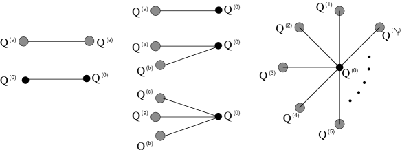
FIG. 1.: The interactions amongst the charges in the CG representation. In this diagram $a\neq b\neq c\neq 0$. The charges can interact only amongst themselves (diagrams furthest left), or with the $Q^{(0)}$ charge.

B Physical Interpretation of Charges

Expression (15) clearly shows that the statistical ensemble of particles interact according to the Coulomb law $\sim|x-y|^{-1}$ in static (time-independent) configurations ( $\sim|x-y|^{-2}$ for time varying ones). An immediate suspicion following from this observation is that these particles carry a magnetic and/or electric charge, since charges of that type interact precisely in the above manner. Due to the direct interaction of the $\theta$-angle and the charges, $Q^{(0)}$, associated with the singlet field, $\phi$, it is quite plausible that they may in fact have a magnetic nature. This suspicion will be corroborated in a moment. Furthermore, since there are several species of charges in the CG picture, a natural question is, “What is the physical relevance of the remaining flavor non-singlet charges $Q^{(a\neq 0)}$?” Evidence of their magnetic nature is found by noting that the VEV’s, $\langle\phi_{a}(\theta)\rangle$, of these fields do in fact depend on the $\theta$-angle. The implication is that all charge species, not only the one dual to the singlet field, have a magnetic origin and are connected to monopoles. Unfortunately, a precise relation of the charges dual to the non-singlet fields and monopole charges is still missing.

As alluded to above, a precise relationship of the $Q^{(0)}$ charges and magnetic monopoles can be made. However, in order to prevent a long interruption in the presentation, only the simplest identifications will be given here, while the interested reader is referred to Appendix B for further detailed discussions. The charge $Q^{(0)}$ was originally introduced in a very formal manner so that the QCD effective low energy Lagrangian (2) can be written in the dual CG form (15). Now the physical content behind these manipulations will be given.

To begin, consider the $SU(2)$ Georgi-Glashow model in the weak coupling regime, with a $\theta$-term, and let the scalar $\Phi^{a}$ have a large VEV. The monopole solution can be constructed explicitly and the so-called Witten effect [19], where the monopole acquires an electrical charge, takes place. Let $N$ denote the generator of large gauge transformations corresponding to rotations in the $U(1)$ subgroup of $SU(2)$ picked out by the gauge field, i.e. rotations in $SU(2)$ about the axis $n^{a}=\frac{\Phi^{a}}{|\Phi^{a}|}$. Rotations by an angle of $2\pi$ about this axis must yield the identity for arbitrary configurations, which implies [19] that the magnetic monopoles carry an electric charge proportional to $\theta$. Indeed,

$$1=e^{i2\pi N}=e^{i2\pi\frac{Q}{e}-i\theta\frac{eM}{4\pi}},$$ (16)

where,

$$M=\frac{1}{v}\int d^{3}xD_{i}\Phi^{a}B_{i}^{a},\quad Q=\frac{1}{v}\int d^{3}xD_{i}\Phi^{a}E_{i}^{a},$$ (17)

are the magnetic and electric charge operators respectively, expressed in terms of the original fields, and $v$ is the VEV of $\Phi^{a}$ at infinity. The combination $\frac{eM}{4\pi}=n_{m}$ in Eq. (16) is an integer and determines the magnetic charge of the configuration. As usual, it is assumed that (16) remains correct in the strong coupling regime when $v$ is not large and/or in the more radical case when $\Phi^{a}$ is not present in the original formulation. Indeed, as explained in [3] the existence of $\Phi^{a}$ is not essential and some effective fields may play its role. One finds that monopoles do exist and the Witten effect expressed by formula (16) remains unaltered even when monopoles appear as singularities in the course of the gauge fixing procedure as described in [3].

Restricting attention to terms which are proportional to the $\theta$-parameter, a comparison between the CG representation, Eq.(15), and Eq.(16) will now be carried out. From the CG the relevant term is the total charge, $Q^{(0)}_{T}$, of the configuration, while in Eq.(16) the relevant factor is the total magnetic charge $\frac{eM}{4\pi}$ for each time slice. The following identification is then made,

$$Q^{0}_{T}=\frac{eM}{4\pi}=n_{m}\in{\rm Z\!\!Z}.$$ (18)

A non-trivial check on this identification can be made by noticing that the $Q^{(0)}$ species are fractionally charged $Q^{(0)}\sim 1/N_{c}$, while the total charge $Q^{(0)}_{T}$is forced to be integer. This follows from the constraint that the difference in the number of positive and negative charges of species $Q^{(0)}$ must be an integer multiple of $p\sim N_{c}$ (see discussions after (15)) and this behaviour is identical to the that of the total magnetic charge.

From these simple observations one can immediately deduce that our fractional magnetic charges $Q^{(0)}$ cannot be related to any semi-classical solutions, which can carry only integer charges; rather, configurations with fractional magnetic charges should have pure quantum origin. Of course, this is a simplified explanation of the identification between the charges $Q^{(0)}$ from (15) and the physical magnetic charges. To make this correspondence more precise the transformation properties of each relevant degree of freedom under a large gauge transformation must be computed and the details of such a calculation can be found in Appendix B.

As already mentioned, the charges $Q^{(a\neq 0)}$ are also suspected to carry magnetic charge, however, a precise statement cannot be made because the large gauge transformations are sensitive only to the singlet combination of fields $\phi$ and consequently only to the dual charge $Q^{(0)}$.

It is interesting to note that a similar phenomenon in the two-dimensional $O(3)~{}\sigma$-model (more generally, in $CP^{N}$ models) has been known for a long time[20]. Namely, an exact accounting and resummation of the $n$-instanton solutions maps the original problem to a $2d$-CG with fractional charges (the so-called instanton-quarks); however, the total topological charge of each configuration is always integer. In that case, it is clear that the quantum fluctuations completely reconstruct all degrees of freedom: each instanton is essentially a superposition of $N_{c}$ instanton-quarks such that, locally, they appear as fractionally charged particles. This superposition is quite nontrivial; however, it is stable under small fluctuations and eventually becomes the only relevant degree of freedom. Indeed, the corresponding two-dimensional CG of the instanton-quarks can be rewritten as a quantum field theory with effective Lagrangian given by the SG model where the dynamics is carried by some effective field $\phi$ [20]. This effective SG Lagrangian describes confinement (mass-gap) and many other important properties of the $O(3)~{}\sigma$-model quite well. Our CG system with fractional magnetic charges, $Q^{(0)}\sim 1/p\sim 1/N_{c}$, is very similar to the situation described above. The difference with [20] is the starting point. In the case of the $O(3)~{}\sigma$-model the statistical-mechanical problem was reduced to some low-energy Lagrangian. However, in the present case we start from the low-energy Lagrangian and a statistical-mechanical model of fractional magnetic monopoles is derived.

Until now, the integers $p$ and $q$ have been considered as free parameters in the theory, and can only be fixed by an explicit dynamical calculation. The only constraint on these parameters has been that in the large $N_{c}$ limit their ratio satisfies $q/p\sim 1/N_{c}$ so that the $U(1)$ problem is resolved. An argument which supports a particular choice for these arguments will now be given. Recall that $q/p$ is related to the $\theta$ dependence of physical observables (such as the vacuum energy $E_{vac}(\theta)$ as can be seen from Eq.(6)). In particular, an observable with expectation value $\sim\exp(i\frac{\theta}{N_{c}})$ corresponds to $q=1$, $p=N_{c}$. The analysis of softly broken SUSY theories [5] strongly suggests that this choice of parameters, $q=1$ and $p=N_{c}$, is in fact correct even for non-supersymmetric models. In this case the number of integrations over $d^{4}x_{i}^{(0)}$ in Eq.(13) exactly equals $4N_{c}k$, where $k$ is an arbitrary integer (not to be confused with the summation parameter appearing in the partition function). This is a direct consequence of the fact that the number of species $Q^{(0)}$ must be an integer multiple of $N_{c}$. This number, $4N_{c}k$ exactly corresponds to the number of zero modes in the $k$-instanton background[21], and, correspondingly, to a number of collective variables associated with these zero modes. In other words, $4N_{c}k$ coordinates $x_{i}^{(0)}$ describe the collective coordinate integration measure of the $k$-instanton solution.

Motivated by the analysis of the two-dimensional $\sigma$-model in [20] and by the above observation regarding the number of collective variables $4N_{c}k$ mentioned above, we conjecture that at large distances our particles, $Q^{(0)}$, with fractional magnetic (and electric for $\theta\neq 0$) charges are indeed the instanton-quarks (i.e. these are related to instantons) suspected long ago [7]. One immediate objection to this conjecture is that since it has long been known (see e.g. [22]) that instantons can explain most low energy QCD phenomenology (chiral symmetry breaking, resolution of the $U(1)$ problem, spectrum, etc) with the exception of its most important property –confinement; and we claim that our magnetic monopoles, $Q^{(0)}$, are instanton-quarks and yet also claim that confinement arises in this picture (they will Bose-condense, see section IV); how can this be consistent? This seeming objection is answered by noting that it in the dilute gas approximation, when the instantons and anti-instantons are well separated and maintain their individual properties (sizes, positions, orientations), quark confinement can not be described. However, the lessons from the two-dimensional $\sigma$ model [20] teaches us that in strongly coupled theories the instantons and anti-instantons lose their individual properties (instantons will “melt”) their sizes become very large and they overlap. If this happens, the description in terms of the instantons and anti-instantons is not appropriate any more, and alternative degrees of freedom should be used to describe the physics. The relevant description is that of instanton-quarks (which, according to our conjecture, are particles with monopole charges $Q^{(0)}$). Further to this point, lattice simulations do not contradict this picture where large instantons induce the magnetic monopole loops forming large clusters, see e.g.[23] and references therein. Also, the connection between monopoles and instantons on the classical level is not a very new idea [24]. Indeed, quite recently, such a relation was established for the periodic instantons (also called calorons) defined on $R^{3}\times S^{1}$ in the presence of a Wilson line [25]. Furthermore, a similar relation was seen in the study of Abelian projection for instantons [26, 27], albeit at the classical level. In particular, Brower et. al. [27] demonstrated that the instanton’s topological charge, $Q$, is given in terms of the charge, $M$, of the monopole, which forms the monopole loop, by the expression $Q=\frac{eM}{4\pi}$. This formula is very similar to our relation (18), where the total topological charge, $Q^{(0)}_{T}$, for a configuration containing a number of particles, $\{Q^{(0)}_{i}\}$, described by the system (15) was identified with the total magnetic charge for each time slice for the same configuration. In spite of this similarity, the physical interpretation of this relation is quite different for these two cases. In the former case it is an identity for a configuration with integer monopole and topological charges satisfying the classical equations of motion; while in the latter case it is a relation for a configuration of the fractionally charged monopoles and topological charges (fractional) for the instanton quarks (which presumably appear after integration over quantum fluctuations in the multi-instanton background). However, given that the instantons at the classical level, and the instanton-quarks at the quantum level both have similar relations suggests that our conjecture is possibly correct. Additional supporting arguments based on the instanton measure for arbitrary gauge groups are given in our concluding remarks.

As a last remark regarding our conjecture, note that the QCD effective Lagrangian (7), at $\theta=0$, is invariant under $CP$ transformations; consequently, the CG representation (13) is also invariant under $CP$ at $\theta=0$. This implies that only when instantons and anti-instantons are taken into account can the statistical ensemble of charges be equivalent, at large distances, to a statistical ensemble of instanton-quarks. If either are left out of the description $CP$ symmetry is broken. The same conclusion also follows from the fact that the partition function, (13), is non-zero in the chiral limit $m_{a}=0$ . Such a behaviour of the partition function implies that our system (13) can be equivalent to the statistical ensemble of the instanton-quarks if and only if both instantons and anti-instantons are present in the system, and there is no excess of the topological charge (for $\theta=0$) which, otherwise, would lead to the chiral suppression of the partition function.

IV Operators

In the previous section, a CG representation which describes the low energy dynamics of the $QCD$ action was derived. The charges were found to have magnetic properties, and the charge species, $Q^{(0)}$, dual to the singlet field, $\phi$, was explicitly identified as magnetic monopoles. However, the formal mapping from the SG description to the CG description, (2) to (15), is not very useful if the dynamics of the fields and charges are not understood. In order to understand the long-distance features of the theory, the manner in which the various charge species behave must be investigated. In particular, if the magnetic charges Bose-condense, this indicates the onset of quark confinement. To investigate the possibility for such a condensation an expression for the magnetic charge creation operator, ${\cal M}$, must be found and its VEV (magnetization) calculated. In this section the magnetization $\langle{\cal M}\rangle$ will be demonstrated to be non-vanishing; consequently, the theory is in the confining phase. Of course, this is not a proof of confinement in $QCD$ because the effective action was constructed under the assumption that the system is in the confining phase, i.e. (2) contains only colorless degrees of freedom. In spite of this, the result is quite nontrivial and can be considered as a self-consistency check of our identifications. In addition, it provides a very nice intuitive picture of the origin of the confinement in $QCD$.

A Charge Creation

Consider inserting a charge, ${\bf q}_{0}=\pm\frac{q}{p}$, of species $Q^{(0)}$ in the bulk at the point ${\bf X}$. To accommodate this insertion, the partition function must be altered by restricting, say, the coordinate $x^{(0)}_{0}={\bf X}$ and $Q^{(0)}_{0}={\bf q}_{0}$. Tracing the steps in the previous section in reverse order with this restriction leads to the appropriate operator equivalence. However, it is simpler state the result and then demonstrate that it is correct. The operator equivalence, which is proven correct shortly, is,

$${\cal M}({\bf q}_{0},{\bf X})={\rm e}^{i{\bf q}_{0}\left(\phi({\bf X})-\theta+2\pi n+2\pi\frac{p}{q}k\right)},$$ (19)

where ${\cal M}$ denotes the operator which inserts the charge in the bulk. The singlet combination $\phi$ naturally appears here since $Q^{(0)}$ is dual to $\phi$, while the appearance of $\theta,n$ and $k$ appear due to the manner in which $Q^{(0)}$ was introduced originally (see Eq. (11)). Clearly this operator must be inserted under the summations over $n$ and $k$. On inserting (19) into the partition function and performing the series expansion in $E$ and $m_{a}$ then introducing the ${\rm Z\!\!Z}_{2}$ valued fields, as before, the modified CG action is arrived at,

$${\rm e}^{-S_{CG}} = \Bigg{\langle}\left({\rm e}^{i\sum_{b=1}^{M_{0}}Q^{(0)}_{b}\left(\phi(x^{(0)}_{b})-\theta+2\pi n+2\pi\frac{p}{q}k\right)}\prod_{a=1}^{{N_{f}}}{\rm e}^{i\sum_{b=1}^{M_{a}}Q^{(a)}_{b}\phi_{a}(x^{(a)}_{b})}\right){\rm e}^{i{\bf q}_{0}\left(\phi({\bf X})-\theta+2\pi n+2\pi\frac{p}{q}k\right)}\Bigg{\rangle}$$ (20)

The term appearing outside the inner parenthesis is the suggested operator for the creation of monopoles. Since ${\bf X}$ and ${\bf q}_{0}$ are not being summed over, this term will act as a source for a fixed charge at a fixed position. Collecting this term with the first term and performing the functional integrals over the scalar fields, demonstrates that ${\bf q}_{0}$ will interact within the statistical model precisely in the form of charge species $Q^{(0)}$ with the exception that its charge and position is not being summed over. Consequently, the operator relation (19) is proven to hold.

The insertion of any other charge species $Q^{(a\neq 0)}$ can be found via an analogous method, and the operators for these charge species are found to be,

$${\cal M}({{\bf q}_{a}},{\bf X})={\rm e}^{i{\bf q}_{a}\phi_{a}({\bf X})}$$ (21)

Notice that (19) explicitly depends on $\theta$, $n$, $k$ and the singlet combination $\phi$, while (21) only depends on the scalar field of its own species, $\phi_{a}$, and not on any other parameters in the theory. This is of course a consequence of $Q^{(0)}$ being associated with monopoles and must transform correspondingly under large gauge transformations. Furthermore, the manner in which the singlet field, $\phi$, appears in (19) allows the further identification of $\phi$ in the CG representation as the magnetic scalar potential.

Now that the relevant operator relations have been identified, questions about the dynamical nature of the system can be asked. The most pressing one being, “Does the operator which creates a charge have a non-zero expectation value?” This is a difficult question to answer in the CG representation, however, in the dual SG representation an answer at the semi-classical level can be given. Its solution, however, requires a knowledge of the VEV’s of the phases of the chiral condensates, $\langle\phi_{a}\rangle$, such that at the semi-classical level $\langle{\cal M}\rangle\simeq{\rm e}^{i{\bf q}_{a}\langle\phi_{a}\rangle}$, and the problem is reduced to the calculation of $\langle\phi_{a}\rangle$. These VEV’s can be found by the minimization of the effective potential (7), and are given by the equations[12],

$$\sin\left(\frac{q}{p}(\langle\phi\rangle-\theta)\right)=-\frac{p}{q}\frac{m_{a}}{E}\sin\langle\phi_{a}\rangle,~{}~{}~{}~{}~{}~{}~{}~{}\phi\equiv{\rm Tr}~{}U=\sum_{a=1}^{N_{f}}\phi_{a},~{}~{}~{}~{}~{}~{}~{}~{}a=1,\dots N_{f}$$ (22)

where the potential has been chosen to be in the particular branch $k=0$. In the limit of equal quark masses, $m_{a}=m$, and assuming $\frac{m}{E}\ll 1$, the system can be solved perturbatively, and to lowest order the VEV’s are: $\langle\phi_{a}\rangle\simeq\frac{\theta}{N_{f}}$ for small $\theta$. Earlier on it was mentioned that the VEV’s of all components of the chiral condensate acquire dependence on the $\theta$-angle and this is now explicitly demonstrated. The suspicion of the magnetic origin of the non-singlet fields can now be justified somewhat, although an explicit construction, as in the case of the singlet field, is still missing. By inserting these VEV’s into the expressions for the charge creation operators the magnetization at the semi-classical level can be evaluated,

$$\langle{\cal M}({\bf q}_{a},{\bf X})\rangle\sim\left\{\begin{array}[]{ll}1&a=0\cr e^{i\frac{\theta}{N_{f}}}&a\neq 0.\end{array}\right.$$ (25)

From Eq. (25) one can clearly see that operator ${\cal M}$ is the order parameter of the system and its nonzero VEV implies the condensation of monopoles (dyons for non-zero $\theta$). Eventually this condensation leads to confinement (oblique confinement for non-zero $\theta$) in the system.

To close this section note that the phase of the order parameter $\langle{\cal M}\rangle$ (25) which labels different vacua in the CG representation (13) is determined by the same equation (22) describing the chiral condensate phases in SG representation (7), which is the conventional description of low-energy QCD in terms of the chiral condensates. The physical meaning of the phases, $\phi_{a}$, presented in the CG representation (13) and in the effective Lagrangian approach (7) is, however, quite different. In the former case they represent the magnetic scalar potential; while in the latter case they are the phases of the chiral condensate. It is quite remarkable that in spite of the very different physical interpretations suggested by the two (dual) approaches lead to the same classification of vacua. One final remark is that generalizations of our calculations of $\langle{\cal M}({\bf q}_{a},{\bf X})\rangle$ for the case of different branches, arbitrary $\theta$ and non-equal quark masses is quite straightforward, and reduces to the solution of Eq. (22) for the phases $\langle\phi_{a}\rangle$. The corresponding analysis has been carried out in [12] and it is not repeated here.

B Background Fields and Wilson Loop Operator

As demonstrated in the previous section, the VEV of magnetization is non-zero, $\langle{\cal M}({{\bf q}_{0}},{\bf X})\rangle\neq 0$; therefore, our system is in the confinement phase as expected. Consequently, the VEV of the Wilson loop $\langle W\rangle$ must show an area law dependence, and it is interesting to find an explicit form of the corresponding Wilson loop insertion in the SG or CG representation. Naively this seems like a hopeless goal, because the starting point, the effective low-energy QCD Lagrangian, does not contain any fundamental degrees of freedom (gluons and quarks) in terms of which the Wilson operator is defined. Nevertheless, as will be seen in a moment, the corresponding Wilson loop insertion operator can be recovered. The key point in this correspondence is again the identification of our charges $Q^{(0)}$ with the physical magnetic charges, Eq. (18). Once this identification is made, the singlet field, $\phi$, in the expression (19) for the magnetic creation operator is interpreted as the magnetic scalar potential such that ${\cal M}({q_{0}},{\bf X})={\rm e}^{iq_{0}\phi({\bf X})}$ represents the interaction energy of a monopole of (fractional) charge $q_{0}$ at position ${\bf X}$ in the presence of the potential of other monopoles. With this identification it is quite obvious what kind of replacement in our formulae (7) and (13) should be made in order to insert a Wilson loop operator. Physics suggests the following picture: For each given time-slice, $x_{0}$, the Wilson loop inserted (at $(x_{1},x_{2})$ plane) into the monopole plasma behaves like a sheet of magnetic dipoles, and produces at large distance from the sheet a dipole magnetic field. The monopoles of the vacuum plasma, however, are polarized by this dipole field and react to produce a dipole field to try to cancel the field from the sheet. Therefore, this interaction of between a source with magnetic charges from the system changes the magnetic scalar potential $\phi$. This change, however occurs only in the thin region where the magnetic plasma of the system does not cancel the field from the sheet. The thickness of this region is order $E^{-1}$, the only dimensional relevant parameter in the system. Therefore, the Wilson loop insertion changes the magnetic scalar potential, $\phi$, by $\phi+\eta$ where $\eta$ is an addition to the magnetic scalar potential due to a dipole layer of unit strength on the sheet $S$ represented by the Wilson surface. The key point is that even though gauge fields are not present in our description, through the identifications of the charges as magnetic monopoles, just enough information about them is encoded in the magnetic scalar potential, $\phi$, to obtain interesting properties. The transformation property of $\phi$ under the Wilson loop insertion, as explained above, is $\phi\rightarrow\phi+\eta$. The function $\eta(x)$ has a discontinuity of $4\pi$ when the point $x$ crosses the surface bounded by the Wilson loop for each given time slice. In a real physical situation the dipole layer is not infinitely thin (as mentioned above it is order of $E^{-1}$); however, incorporating the finite thickness is beyond the present analysis.

An explicit representation for the appropriate source term will now be constructed. It will be explicitly demonstrated that such a source interacts with the magnetic charges $Q^{(0)}$ exactly in the same manner as the $\phi$ field, $\sim{\rm e}^{iQ^{(0)}\eta}$. Therefore, the $\eta$ source insertion can be identified with an appropriate change in the magnetic scalar potential $\phi\rightarrow\phi+\eta$. But, as explained above, the Wilson loop insertion must also lead to precisely this kind of shift $\phi\rightarrow\phi+\eta$ in SG (7) or CG (13) representation.

The insertion of background dependence is furnished by altering the Gaussian weighting (8) to include source terms,

$$\langle\dots\rangle=\sum_{k=0}^{p-1}\sum_{n=-\infty}^{\infty}\int{\cal D}\phi_{a}~{}\dots~{}{\rm e}^{-g^{2}\int d^{4}x\left\{\frac{1}{2}({\vec{\nabla}}\phi_{a})^{2}+\phi_{a}\Box\eta_{a}^{(0)}\right\}}$$ (26)

The classical equations of motion are of course modified by this insertion, and with appropriate choices of the source fields, $\eta_{a}^{(0)}$, the classical solution can be made kink like, for example. However, $\eta_{a}^{(0)}$ will not be constrained at this moment, and any source (Wilson loop, domain wall or anything else) can be described by this modification. Of course, it is interesting to study what this modification implies for the CG representation. On expanding the partition function in powers of $E$ and $m_{a}$, and introducing the ${\rm Z\!\!Z}_{2}$ valued charge fields one arrives at precisely equation (13) where the angled brackets are the modified ones above. Performing the functional integral posses no difficulty and one arrives at the CG representation,

$$Z = \sum_{\{M_{0},\dots,M_{N_{f}}\}=0}^{\infty}\frac{(E/2)^{M_{0}}}{M_{0}!}\frac{(m_{1}/2)^{M_{1}}}{M_{1}!}\dots\frac{(m_{N_{f}}/2)^{M_{N_{f}}}}{M_{N_{f}}!}\int\left(dx^{(0)}_{1}\dots dx^{(0)}_{M_{0}}\right)\dots\left(dx^{(N_{f})}_{1}\dots dx^{(N_{f})}_{M_{N_{f}}}\right)$$ (28)

$$\hskip 28.45274pt\times\sum_{\stackrel{{\scriptstyle\scriptstyle Q^{(0)}_{i}=\pm\frac{q}{p}}}{{\{Q^{(1)}_{i},\dots,Q^{({N_{f}})}_{i}\}=\pm 1}}}{\rm e}^{-S_{CG}-\frac{g^{2}}{2}\int d^{4}x~{}\eta_{a}\Box\eta_{a}}{\rm e}^{i\sum_{b=1}^{M_{0}}Q^{(0)}_{b}\eta(x^{(0)}_{b})}\prod_{a=1}^{N_{f}}{\rm e}^{i\sum_{b=1}^{M_{a}}Q^{(a)}_{b}\eta_{a}(x^{(a)}_{b})}$$

In the above, $S_{CG}$ is the CG action containing the interactions of the charges and is unaltered from its form given in equation (15), also $\eta\equiv\eta_{1}+\dots+\eta_{N_{f}}$. This then allows the identification of the operator, in the CG representation, which introduces a source for the classical equations of motion of the phases of the chiral condensates,

$${\cal C}(\eta_{a})={\rm e}^{-\frac{g^{2}}{2}\int d^{4}x~{}\eta_{a}\Box\eta_{a}}~{}{\rm e}^{i\sum_{b=1}^{M_{0}}Q^{(0)}\eta(x^{(0)}_{b})}\prod_{a=1}^{N_{f}}{\rm e}^{i\sum_{b=1}^{M_{a}}Q^{(a)}_{b}\eta_{a}(x^{(a)}_{b})}$$ (29)

in this formula the term ${\rm e}^{-\frac{g^{2}}{2}\int d^{4}x~{}\eta_{a}\Box\eta_{a}}$ represents a self-interaction of the source with itself, it is irrelevant for the present purposes and will be omitted in the analysis. The second term in (29) is much more interesting and gives a very simple prescription for the insertion of any source. If one wants to insert some classical field configuration (source) in the original formulation, then in the CG picture one need only introduce a phase factor which gives rise to a source term for that background - all interactions among the charges remain unaltered. The charges simply interact with the source field just as if it were an external magnetic field, each charges species, $Q^{(a\neq 0)}$, interacts with the source component with which it is associated to, $\eta_{a}$, while the singlet charge species $Q^{(0)}$ interacts with all of the background fields. The special form of the SG action is what admits this very simple picture and is at the heart of the CG representation itself. Consequently, it is expected that the analysis carried out here has wide applicability and can be applied for any kind of sources.

In deriving (29) no assumptions about the source fields $\eta_{a}$ have been made. The remainder of this section will be devoted to the most interesting source - the Wilson loop operator insertion. As argued above, any source can be accounted for by the shift $\phi\rightarrow\phi+\eta$, and the Wilson loop operator insertion is no exception. Our problem, therefore, is reduced to the calculation of a difference in magnetic scalar potential due to the insertion of this specific source. Before dealing with the $4d$ case, some relevant formulae from the $3d$ case, where the physics is well understood, will be reviewed; then the appropriate generalizations to the $4d$ case will be made. The reason that the $3d$ analysis can be easily generalized to the $4d$ case is that in both cases the interactions between particles in the CG representation (15) is determined by the relevant Greens function ($1/|x-y|$ or $1/(x-y)^{2}$ respectively); consequently, the Wilson loop insertion in the CG representation should be expressible in terms of the appropriate Greens function. Hence, if the Wilson loop insertion operator in $3d$ can be expressed exclusively in terms of the $3d$ Greens function, $1/|x-y|$, the transition from three to four dimensions will be furnished by the replacement of the $3d$ Greens function by the $4d$ Greens function such that the static limit is reproduced. In addition, it is expected that the Wilson loop insertion is a Lorentz-covariant expression.

Recall that in the well-understood $QED_{3}$, Polyakov[1] demonstrated that the expectation value of a Wilson loop operator can be written in terms of a CG with the insertion of the operator,

$$\langle W\rangle\sim{\rm e}^{\frac{i}{2}\eta(x,C)},~{}~{}~{}\eta(x,C)=\int_{\Sigma_{C}}d^{2}\sigma_{\mu}(y)\frac{(x-y)_{\mu}}{|x-y|^{3}}=-\int_{\Sigma_{C}}d^{2}\sigma_{\mu\nu}(y)\frac{1}{2}\epsilon^{\mu\nu\lambda}\partial_{\lambda}\frac{1}{|x-y|}$$ (30)

where the factor of $1/2$ appearing in the exponential is due to the external quarks being in the fundamental representation; $\eta(x,C)$ is the solid angle subtended by the loop $C$ at the point $x$; and $\Sigma_{C}$ is an arbitrary surface bounded by the counter $C$. For simplicity, $\Sigma_{C}$ will be assumed to lie in the $(x_{1},x_{2})$ plane. In the case of infinitely large Wilson loops, the solid angle is $2\pi$ below the surface, and changes discontinuously across the loop to $-2\pi$. Physically $\eta(x,C)$ is the magnetic scalar potential due to a dipole layer of unit strength on the sheet $\Sigma_{C}$. As expected, formula (30) can be expressed exclusively in terms of the $3d$ Greens function which is the only relevant element of the CG representation. Also note that, if the fractional monopole charges of strength $1/N$ were present in the system, an additional factor of $1/N$ would appear in the expression for $\eta(x,C)$ in Eq.(30). From Eq. (30), $\Box\eta$ can be easily computed,

$$\Box\eta=4\pi\Theta_{\Sigma_{C}}(x_{1},x_{2})\delta^{\prime}(x_{3}),~{}~{}~{}\eta=2\pi\Theta_{\Sigma_{C}}(x_{1},x_{2}){\rm sgn}(x_{3}),$$ (31)

where $\Theta_{\Sigma_{C}}(x_{1},x_{2})$ is unity within the surface $\Sigma_{C}$ and zero outside.

As argued above, the transition from $3d$ to $4d$ is realized by the replacement

$$\frac{1}{4\pi|x-y|}\rightarrow\frac{1}{2\pi^{2}(x_{\mu}-y_{\mu})^{2}},~{}~{}~{}1\rightarrow\int dt,$$ (32)

where the numerical factors, $4\pi$ and $2\pi^{2}$, are the volumes of the two- and three- dimensional unit spheres respectively, and appear so that the Green functions are properly normalized, $\Box G(xy)=-\delta(x-y)$. Furthermore, an integration over all time-slices must be included to complete the transition to $4d$. Carrying out the replacements (32) in Eq. (30), the following expression for $\eta(x,C)$ written in the covariant $4$ dimensional form is arrived at,

$$\eta(x,C)=-\frac{1}{\pi}\int_{\Sigma_{C}}d^{2}\sigma_{\mu\nu}(y)\oint dx_{\sigma}\epsilon^{\mu\nu\lambda\sigma}\partial_{\lambda}\frac{1}{(x-y)^{2}},$$ (33)

here the integration over time-slices $\int dt$ for a static particle was replaced by the integration along an arbitrary trajectory of a particle, $\epsilon^{\mu\nu\lambda}dt\rightarrow\epsilon^{\mu\nu\lambda\sigma}\oint dx_{\sigma}$. In the static limit, (33) is reduced to expression (30) as it must by construction. It is interesting to note that Eq. (33) for $\eta$ (with appropriate normalization) is formally similar to the expression for the linking number of a closed oriented surface $d^{2}\sigma_{\mu\nu}$ and closed oriented curve $\oint dx_{\sigma}$ in four dimensions. However, the surface $\Sigma_{C}$, bounded by the Wilson loop, and a trajectory of the particle are not closed manifolds; nevertheless $\eta$ can be interpreted as measuring a solid angle, in addition $\frac{\eta}{2\pi}$ has an integer-number-discontinuity when a particle crosses the surface $\Sigma_{C}$ analogous to the $3d$ case (30), where for a very large Wilson loop $\frac{\eta}{2\pi}=\pm 1$ just above and just below the surface.

From Eq. (33), $\Box\eta$ can be calculated for the Wilson loop in the $(x_{1},x_{2})$ plane with the following result,

$$\Box\eta=\frac{1}{\pi}(2\pi^{2})\int_{\Sigma_{C}}d^{2}\sigma_{\mu\nu}(y)\oint dy_{\sigma}\epsilon^{\mu\nu\lambda\sigma}\partial_{\lambda}\delta^{4}(x-y)\rightarrow 4\pi\Theta_{\Sigma}(x_{1},x_{2})\int dy_{\lambda}\epsilon^{\lambda\sigma}\partial_{\sigma}\delta^{2}(x-y),~{}~{}\lambda,\sigma=0,3,$$ (34)

and is the final expression for the source of a Wilson loop in four dimensions. For the static case, the integration over $t$ can be carried out and the above expression reduces to the $3d$ result found in Eq. (31). For very large Wilson surfaces, Eq. (34) suggests the following simplified expression for $\eta$,

$$\eta=\Theta_{\Sigma}(x_{1},x_{2})\int dy_{\lambda}\epsilon^{\lambda\sigma}\partial_{\sigma}\ln(x-y)^{2},~{}~{}\lambda,\sigma=0,3.$$ (35)

Indeed, applying the operator $\Box$ to Eq. (35), and taking into account the relation $\Box\ln(x-y)^{2}=4\pi\delta^{2}(x-y)$, reproduces Eq. (34). Equation (34) explicitly shows that $\eta/(2\pi)$ has a discontinuity whenever a particle crosses the surface. This is precisely the property of the Wilson loop insertion. Drawing attention to the behaviour in the SG picture, Eq. (7), the Wilson loop insertion corresponds to the shift $\phi\rightarrow\phi+\eta$ in the flavor singlet term of the potential (7): $E\cos\left(\frac{q}{p}\left(\phi+\eta-\theta+2\pi n\right)+2\pi k\right)$.

The above discussions should have convinced the reader that although the effective SG action for low energy QCD does not contain the fundamental gauge degrees of freedom, it is possible to recover the Wilson loop insertion operator by inserting the appropriate source term. The two key points in making such a correspondence were:

1. $Q^{(0)}$ was identified with the physical magnetic charges; consequently, the singlet combination of fields, $\phi$, was identified with the physical magnetic scalar potential

2. Confinement is realized in this system through the condensation of the magnetic charges $Q^{(0)}$ such that $\langle{\cal M}\rangle\neq 0$. In this case the insertion of the Wilson loop in the monopole plasma leads to a shift $\phi\rightarrow\phi+\eta$ of the corresponding magnetic scalar potential as demonstrated above (29).

One further point is that since the species $Q^{(0)}$ have fractional charge of strength $1/N_{c}$, this additional factor should be introduced in front of Eq. (33).

Even though the insertion of the Wilson loop operator in the CG representation is now understood, the calculation of its VEV is much more difficult in comparison with Polyakov’s model [1]. The fundamental difference is related to the fact that in Polyakov’s case the weak coupling regime is justified, and the classical action dominates over the contributions from one loop fluctuations. In the present case the only relevant dimensional parameter is the vacuum energy, $E\sim\Lambda_{QCD}$, all other parameters are expressed in terms of $E$ and are of the same order of magnitude; as such, there are no small parameters in the problem. Nevertheless, the VEV of the Wilson loop can be estimated in the semi-classical approximation analogous to Ref. [1]. In this case for each given time-slice, the problem is effectively a $3d$ problem described in [1] where the area law has been demonstrated $\langle W\rangle\sim\exp{(-S)}$ with calculable string tension. In our $4d$ case, it is also expected that $\langle W\rangle$ demonstrates the area law in agreement with our earlier calculation of the magnetization, $\langle{\cal M}\rangle\neq 0$; however, an explicit calculation is still lacking.

To conclude this section, we note that a second important source appears in this system due to the existence of domain wall solutions to the equations of motion derived from (7). These domain walls interpolate between vacuum states labeled by the parameter $k$, and were discussed in some detail in [17]. Similar domain walls are known to exist in supersymmetric models, and are reviewed quite thoroughly in [5]. Recently, Witten conjectured [6] that in the large $N$ limit the domain walls connecting two vacua labeled by $k$ and $k+1$ appear to be object that are not solitons, from the string viewpoint, but rather look like $D$-branes on which the string should be able to end. Such $D$-brane-like domain walls have recently appeared in [6] in the context of the AdS/CFT correspondence. In fact, our CG picture seems to indicate that such a phenomenon takes place in QCD as well. Indeed, a distinguishable property of $D$-branes is that in large-$N$ limit its tension is $\sim N$. Domain walls described in[17] have exactly this property. Additional support in favor of this identification comes from our demonstration of the condensation of fractionally charged $\sim a/N$ magnetic particles; which implies that the electric charges in the system could also be fractional and the domain walls support excitations that carry electric charges $\sim 1/N$. Consequently, the chromo-electric flux contained in the open string of the corresponding (non-critical) string theory can end on the QCD $D$-brane.

V Conclusion

The most important “formal result” of this paper is given by Eqs. (13, 15); which we claim is the new representation of low energy QCD (7) that is appropriate for the analysis of the vacuum structure. The correspondence between these two representations is discussed at length in the text. The most important physical (as opposite to the “formal”) result of the paper is formulated as a conjecture described at the end of Section III in which the charges, $Q^{(0)}_{i}$, from the statistical ensemble (13, 15) are identified with the instanton-quarks[7]. If this conjecture is proven correct, enormous progress in our understanding of QCD will have been made. For example, it would fill the missing element of the well-developed instanton picture[22] to include the electric confinement of quarks as a natural consequence of the same well-known BPST-instantons[28],[29] which have been under intensive study since the 70s. Indeed, as discussed in the text, our particles (which are the instanton-quarks, according to the conjecture) gain the magnetic charges which condense, $\langle{\cal M}\rangle\neq 0$. Therefore, the standard ’t Hooft-Mandelstam picture [2] for the confinement would occur due to the instantons.

Various arguments which support this conjecture have been given in the bulk of the text; however, one further reason why we believe this conjecture could be correct will now be presented. Our CG representation implies that the number of integrations $d^{4}x_{i}^{(0)}$ in (13) for each configuration is exactly equal to the number, $M_{0}$, of fractionally charged particles, $Q^{(0)}\sim 1/p$, for that configuration. Due to the fact that the total charge of the configuration is integer, the number $M_{0}$ must be proportional to the denominator of the charge, i.e $\sim p$; while, the fractional charge $Q^{(0)}\sim 1/p$ in the CG representation appears due to the $\theta/p$ dependence in the effective Lagrangian approach (7). Consequently, as long as there is a $\theta/p$ dependence in the SG representation, the number $M_{0}$ must be an integer multiple of $p$, and the total dimensionality of integrations over $d^{4}x_{i}^{(0)}$ is $4M_{0}=4pk$. This is exactly the measure in the multi-instanton background with $p=C_{2}(G)$! The quadratic Casimir operator $C_{2}(G)$ appears here because in SUSY theories this number determines the $\theta/C_{2}(G)$ dependence.

Indeed, it is well known since the work in [30] that the $\theta$ dependence of the gluino condensate $\langle Tr\lambda\lambda\rangle_{\theta}$ in SYM with arbitrary gauge group $G$ is,

$$\langle Tr\lambda\lambda\rangle_{\theta,k}=\langle Tr\lambda\lambda\rangle_{\theta=0}\exp\left(i~{}\frac{\theta+2\pi k}{C_{2}(G)}\right),~{}~{}~{}k=0,1,...,~{}C_{2}(G)-1$$ (36)

where $C_{2}(G)$, the quadratic Casimir operator, becomes equal to the dual Coxeter number when the longest root vectors is normalized to have length one. In particular, $C_{2}(SU(N))=N$, $C_{2}(SO(N))=N-2$, $C_{2}(Sp(2N))=N+1$. Formula (36) implies that for each given $\theta$ there exist $C_{2}(G)$ degenerate vacuum states (which corresponds to the Witten index) for which $\langle Tr\lambda\lambda\rangle$ differs by a phase factor of $\exp\left(i~{}\frac{2\pi k}{c_{2}(G)}\right)$. Then the $\theta$ evolution from $\theta=0$ to $\theta=2\pi$ according to Eq. (36) simply renumbers these states in a cyclic way. The easiest way to understand this result is (roughly speaking) to count the number of gluino zero modes in the one instanton background (it is equal to $2C_{2}(G)$) such that the correlation function $\langle Tr\lambda\lambda,Tr\lambda\lambda,...\rangle_{\theta,k}\sim\exp(i\theta),$ including $C_{2}(G)$ insertions of the operator $Tr\lambda\lambda$ is not zero. Formula (36) then follows from the consideration of this correlation function (for a complete analysis see the original paper [30]). The number of bosonic zero modes is twice as much and equals to $4c_{2}(G)$[21]. The generalization of this result for an arbitrary number, $k$, of instantons is also well known and is given by the formula $4C_{2}(G)k$[21]. These well known results are reviewed here to place emphasis on the one-to- one correspondence between $\theta/C_{2}(G)$ dependence of the physical parameters and the number of zero modes $4C_{2}(G)k$ in the $k$ instanton background. But as argued above, the total dimensionality of integrations over $d^{4}x_{i}^{(0)}$ in our formula (13) exactly equals to this number $4M_{0}=4C_{2}(G)k$, if the $\theta/C_{2}(G)$ dependence in non-supersymmetric gluodynamics remains the same as in SUSY theories. Soft supersymmetry breaking analysis strongly suggests that this is the case[5]. Therefore, our conjecture can be reformulated in the following way: if $\theta/C_{2}(G)$ dependence in non-supersymmetric gluodynamics remains the same as in SYM, our particles (13) could be nothing but the instanton-quarks suspected long ago[7]. The recent paper[31], where it was demonstrated that in SYM the instanton-quarks carry magnetic charges and saturate the gluino condensate, also supports our picture.

As a final concluding remark, at the intuitive level there seems to be a close relationship between our CG representation in terms of Abelian monopoles, $Q_{i}^{(0)}$, and the “Abelian projection” approach [23, 26, 27] as well as the “periodic instanton” analysis [25]. We also feel that there is a close connection with the work of [32] in the description of infra-red QCD physics. Unfortunately, an explicit realization of these correspondences is still missing at the moment; however, the search for such mappings will be the focus of future studies.

VI Acknowledgments

This work is supported in part by the National Science and Engineering Research Council of Canada. S. J. would like to thank the University of British Columbia for financial support through a University Graduate Fellowship.

Appendix A: $\theta$-dependence in the massless limit

In this appendix the $\theta$-dependence of the partition function is proven to vanish in the limit of zero quark masses. This is an absolutely trivial and well-known result of QCD. It is easily understood from the effective Lagrangian approach (7), where the $\theta$ dependence can be eliminated in the chiral limit by the shift $\phi\rightarrow\phi-\theta$. However, it is instructive to understand this $\theta$ independence of $Z$ by direct analysis of the statistical ensemble (15) with nonzero $\theta$ within the CG representation. It will be demonstrated that the $\theta$ independence is recovered in the chiral limit as a consequence of the long range Coulomb interactions. Neglecting the interactions will result in explicit $\theta$ dependence of the partition function, which is clearly unwanted. The first point to notice is that in this limit only configuration which contain the species $Q^{(0)}$ are allowed. This occurs since the mass dependence in the partition function appears as $(m_{a}/2)^{M_{a}}$, for $a\neq 0$, where $M_{a}$ is the number of charges of species $Q^{(a)}$. Therefore in the massless limit the partition function reduces to that of a single charge species $Q^{(0)}$.

For $\theta\neq 0$ it is convenient to label the configurations by the number of positively, $n_{1}$, and number of negatively, $n_{2}$ charged particles (note that for $\theta\neq 0$ the $n_{1}$ and $n_{2}$ need not be equal). In this case the total charge of the configuration $Q^{(0)}_{T}=\sum_{i=1}^{M_{0}}Q^{(0)}_{i}=n_{1}-n_{2}$, while the total number of pseudo-particles $M_{0}=n_{1}+n_{2}$ is fixed and the corresponding contribution, $Z^{(M_{0},Q)}$, to the partition function (15) is,

$$Z^{(M_{0},Q)}(\theta) \equiv \exp(-iQ\theta)\exp(-F^{(M_{0},Q)})$$ (37)

$$= \exp(-iQ\theta)\frac{(E/2)^{M_{0}}}{n_{1}!n_{2}!}\prod_{i=1}^{M_{0}}d^{4}x_{i}~{}\exp\left\{-\sum_{i\neq j}^{M_{0}}\frac{Q_{i}Q_{j}}{|x_{i}-x_{j}|^{2}}\right\}$$ (38)

where, without losing generality, only the first branch with $k=0$ appears here; the superscript $(0)$ on $Q$ has been removed since only a single charge species is present; $E$ is the fugacity of the Coulomb gas; the combinatorical factor $\frac{M_{0}!}{n_{1}!n_{2}!}$ has been introduced for the correct counting of $n_{1}$ identical particles with charge $(+)$ and $n_{2}$ identical particle with charge $(-)$; and,

$$Q\equiv Q^{(0)}_{T}=n_{1}-n_{2},\ \ \ M_{0}=n_{1}+n_{2},\ \ \ Q_{i}=\pm 1,\ \ \ i=1,...M_{0},$$ (39)

For the special case of vanishing $\theta$, the neutrality condition would require $n_{1}=n_{2}$ in the thermo-dynamical limit. Now, if the Coulomb interaction could be ignored, then (38) yields a free energy $F(\theta)\simeq-\log Z(\theta)$ which is a $\theta$-dependent expression. Indeed, the partition function for a noninteracting gas with a fixed total charge $Q$,

$$Z^{Q}(\theta)\equiv\exp(-iQ\theta)\exp(-F^{Q})=\sum_{M_{0}}Z^{(M_{0},Q)}(\theta)\rightarrow\int dM_{0}~{}Z^{(M_{0},Q)}(\theta)$$ (40)

can be obtained by the steepest descent method with respect to $M_{0}$. If the size of the system, $L$, is large, the noninteracting case reduces to,

$$\exp(-F^{Q}) = \int dM_{0}~{}\exp\left(M_{0}\ln(L^{4}E)\right)\times\exp\left\{\frac{M_{0}+Q}{2}\left(\ln\frac{M_{0}+Q}{2}-1\right)-\frac{M_{0}-Q}{2}\left(\ln\frac{M_{0}-Q}{2}-1\right)\right\}$$ (41)

$$\sim \exp(\overline{M}_{0})~{}\exp\left\{-\frac{Q^{2}}{2\overline{M}_{0}}\right\}$$ (42)

where the formula $\ln(k!)\sim k\ln k-k$ has been used, and $\overline{M}_{0}$ is the saddle point determined from the equation,

$$\ln(L^{4}E)=\frac{1}{2}\ln\left\{\frac{{\overline{M}_{0}}^{2}-Q^{2}}{4}\right\},\qquad\frac{Q}{M_{0}}\ll 1,\qquad\overline{M}_{0}\simeq 2L^{4}E$$ (43)

In this approximation of noninteracting particles, the partition function is evaluates to,

$$Z(\theta)\equiv\exp(-F(\theta))\sim\exp(2L^{4}E)\int dQ\exp(-i\theta Q)\exp\left\{-\frac{Q^{2}}{4EL^{4}}\right\}\sim\exp\left\{2EL^{4}\left(1-\frac{\theta^{2}}{2}\right)\right\}$$ (44)

Consequently, the free energy is given by,

$$F(\theta)\simeq-2EL^{4}\left(1-\frac{\theta^{2}}{2}\right),\qquad\theta\ll 1$$ (45)

The evaluation of $Z$ appearing in (44) reveals that the essential terms are those which contain the charges,

$$|Q|\sim EL^{4}\theta,\ \ \ \ \ \ \ \ \ \frac{|Q|}{M_{0}}\sim\theta$$ (46)

and the approximation $Q/M_{0}\ll 1$ can be justified for small $\theta\ll 1$ which will be assumed henceforth. Therefore, as expected, the free energy $F(\theta)$ for the gas of the noninteracting particles explicitly depends on $\theta$.

The discussion now returns to the full long-range interacting Coulomb gas (38). This problem is in all respects very similar to Polyakov’s model[1]. It is known from [33] that the Coulomb interactions in a plasma cannot be ignored in this case. Hence, formula (44) is certainly misleading. In order to derive some estimation for the interacting case, once again the system is placed into a box of size $L$. In this case, excessive charge is deposited on the walls of the box, and the free energy is that of a neutral Debye plasma plus the Coulomb energy, similar to what happens in the well-understood $QED_{3}$ case [33],

$$\exp(-F^{Q})\sim\!\!\int\!\!dM_{0}~{}\exp\left(M_{0}\ln(L^{4}E)\right)\times\exp\left\{\frac{M_{0}+Q}{2}\left(\ln\frac{M_{0}+Q}{2}-1\right)-\frac{M_{0}-Q}{2}\left(\ln\frac{M_{0}-Q}{2}-1\right)-\frac{Q^{2}}{L^{2}}\right\}$$ (47)

The partition function with a fixed total charge $Q$ can now be estimated as in (42,43), with the only difference occurring in the last term which is due to the Coulomb interaction. This term plays a key role in the following integration over all charges $\int dQ$,

$$Z(\theta)\equiv\exp(-F(\theta))\sim\exp(2L^{4}E)\int dQ~{}\exp(-i\theta Q)~{}\exp\left\{-\frac{Q^{2}}{4EL^{4}}\right\}~{}\exp\left\{-\frac{Q^{2}}{L^{2}}\right\}$$ (48)

Taking into account the extra factor $\exp(-\frac{Q^{2}}{L^{2}})$, the charges of the essential configurations behave as,

$$|Q|\sim L^{2}\theta,\ \ \ \ \ \ \frac{Q}{M_{0}}\sim\frac{\theta}{L^{2}}\rightarrow 0~{}~{}at~{}~{}L\rightarrow\infty$$ (49)

consequently,

$$F(\theta)\sim-2EL^{4}+L^{2}\theta^{2}=-2EL^{4}\left\{1-\frac{\theta^{2}}{2L^{2}}\right\}$$ (50)

Thus, as $L\rightarrow\infty$, the free energy $F(\theta)$ in $QCD_{4}$ in the chiral limit does not depend on $\theta$, which is precisely how it should behave and is exactly what is expected from the Sine-Gordon representation (7) of the partition function. It should be emphasized once more that this result is a direct consequence of the strong Coulomb interactions in the system.

Appendix B: Large gauge transformations and monopole charges

In this Appendix the large gauge transformations generated by the operator $N$, as discussed in the text (16), will be elaborated on. It will be demonstrated that such a transformation is equivalent to the identity operator. In the following analysis it will be assumed, along the lines of ‘t Hooft [3], that formula (16) has much more general applicability and is not necessarily constrained to the weak coupling limit of the Georgi-Glashow model where it was originally derived. Due to knowledge of the $\theta$-dependence in the effective low energy potential on both sides of Eq. (16), the magnetic properties of the relevant fields describing the large distance physics will be identified.

The strategy is to begin with the QCD effective anomalous potential before the glue-ball degrees of freedom are integrated out. Next, a large gauge transformation will be performed on this effective potential. It is clear that this operation is equivalent to applying the identity operator; however, in the course of the following calculations, the magnetic and electric properties of the fields making up the effective potential will be identified..

Recall that the effective potential is defined as the Legendre transform of the generating functional for zero momentum correlation functions of the marginal operators $G_{\mu\nu}\tilde{G}_{\mu\nu}$, $G_{\mu\nu}G_{\mu\nu}$ and $m\bar{\Psi}^{i}\Psi^{i}$, see [12],[17] for details. It is a function of the effective zero momentum fields $h,\bar{h}$ which describe the VEV’s of the composite complex fields $H,\bar{H}$,

$$\int dx\,h=\left\langle\int dx\,H\right\rangle\quad,\quad\int dx\,\bar{h}=\left\langle\int dx\,\bar{H}\right\rangle$$

where,

$$H=\frac{1}{2}\left(\frac{\beta(\alpha_{s})}{4\alpha_{s}}G^{2}+i\,\frac{2p}{q}\frac{\alpha_{s}}{4\pi}G\tilde{G}\right)\;,\;\bar{H}=\frac{1}{2}\left(\frac{\beta(\alpha_{s})}{4\alpha_{s}}G^{2}-i\,\frac{2p}{q}\frac{\alpha_{s}}{4\pi}G\tilde{G}\right)\;.$$ (51)

The potential is also function of the unitary matrix $U_{ij}$ corresponding to the $\gamma_{5}$ phases of the chiral condensate: $\langle\bar{\Psi}_{L}^{i}\Psi_{R}^{j}\rangle=-|\langle\bar{\Psi}_{L}\Psi_{R}\rangle|\,U_{ij}$. As explained in Section 2 the corresponding Lagrangian reproduces the chiral and conformal anomalies and also corresponds to the following behavior of the $(2k)^{\rm th}$ derivatives of the vacuum energy in pure gluodynamics,

$$\left.\frac{\partial^{2k}E_{vac}(\theta)}{\partial\,\theta^{2k}}\right|_{\theta=0}\sim\int\prod_{i=1}^{2k}d^{4}x_{i}\langle Q(x_{1})...Q(x_{2k})\rangle\sim\left(\frac{i}{N_{c}}\right)^{2k},$$ (52)

where $Q\sim G_{\mu\nu}{\widetilde{G}}_{\mu\nu}$. This is a consequence of the solution of the $U(1)$ problem when Veneziano ghosts saturate all relevant correlation functions (52) [18].

Our starting point is then the effective QCD potential $W(h,U)$ which in Minkowski space takes the form[12],

$$e^{-iVW(h,U)} = \sum_{n=-\infty}^{+\infty}\sum_{k=0}^{q-1}\exp\left\{-\frac{iV}{4}\left(h\,\log\,\frac{h}{2eE}+\bar{h}\,\log\,\frac{\bar{h}}{2eE}\right)\right.$$ (54)

$$\hskip 71.13188pt+\left.i\pi V\left(k+\frac{q}{p}\,\frac{\theta-i\log Det\,U+2\pi n}{2\pi}\right)\frac{h-\bar{h}}{2i}+\frac{i}{2}V\,{\rm Tr}(MU+h.c.)\right\}\;,$$

where $M={\rm diag}(m_{i}|\langle\bar{\Psi}^{i}\Psi^{i}\rangle|)$ , $V$ is the volume of the system and the complex fields $h,\bar{h}$ are defined as in Eq.(51).

The anomalous effective potential (54) contains both the light chiral fields $U$ and heavy “glue-ball” fields $h\,,\,\bar{h}$, and is therefore not an effective potential in the Wilsonian sense. On the other hand, only the light degrees of freedom, described by the fields $U$ are relevant for the low energy physics. An effective potential for the $U\,,\,\bar{U}$ fields can be obtained by integrating out the $h\,,\,\bar{h}$ fields in Eq.(54). In SUSY models the transition from the effective potential for the $U$, $h$ fields to the effective potential for the $U$ fields, by integrating out the $h\,,\,\bar{h}$ fields, is analogous to the transition from effective Lagrangian [10] for SQCD to the Affleck-Dine-Seiberg [34] low energy effective Lagrangian. The corresponding derivation for QCD was described earlier in [12, 17]. The goal here is to study the properties of the various fields from (54 ) under large gauge transformations. In order to gain an understanding of what changes this large gauge transformation produces, the complex $h,\bar{h}$- fields are parameterized by introducing two real fields $\rho$ and $\omega$,

$$h=2E\,e^{\rho+i\omega}\;\;,\;\;\bar{h}=2E\,e^{\rho-i\omega}\;.$$ (55)

The summation over the integers $n$ in Eq.(54) then enforces the quantization rule due to the Poisson formula,

$$\sum_{n}\exp\left(2\pi in\,\frac{q}{p}\,V\,\frac{h-\bar{h}}{4i}\right)=\sum_{m}\delta\left(\frac{q}{p}\,VEe^{\rho}\,\sin\omega-m\right)\;,$$ (56)

This reflects quantization of the topological charge $Q=\left(\frac{q}{p}\,VEe^{\rho}\,\sin\omega\right)$ which must be an integer, $m$, in the original theory. Applying a large gauge transformation, $T={\rm e}^{i2\pi N}$, then implies that $m$ in Eq. (56) undergoes the shift $m\rightarrow m-1$. Indeed, by definition

$$Z\sim\sum_{n}\sum_{m}\langle n|e^{-S-i\theta Q}|m\rangle,\qquad Q=m-n,$$

where the $|\theta\rangle$ state is the eigenstate of the large gauge transformation operator, $T$, with eigenvalue $e^{-i\theta}$. Consequently, when a large gauge transformation is performed the topological charge of the configuration becomes shifted $Q\rightarrow Q+1$. This corresponds to the replacement $m\rightarrow m-1$ in Eq. (56). It is quite clear that such a replacement does not change any physical content of the theory due to the summation over $m$ in Eq. (56). Therefore, the large gauge transformation is equivalent to the identity operation as expected. However, the transformation properties of the individual fields under such an operation is what needs to be understood. Hence, proceeding further, and using (56), Eq.(54) (with the mass term omitted) is placed in the form,

$$e^{-iVW}=\sum_{m=-\infty}^{+\infty}\sum_{k=0}^{q-1}\delta\left(VE\,\frac{q}{p}\,e^{\rho}\sin\omega-m\right)\,\exp\left\{-iVE\,e^{\rho}(\rho-1)\cos\omega+im\left(\bar{\theta}_{k}+\frac{p}{q}\,\omega\right)\right\}$$ (57)

where,

$$\bar{\theta}_{k}\equiv\theta-i\log Det\,U+2\pi\,\frac{p}{q}\,k\;.$$ (58)

To resolve the constraint imposed by the presence of the $\delta$-function in Eqs.(56),(57), a Lagrange multiplier field, $\Phi$, is introduced,

$$\delta(VE\,\frac{q}{p}\,e^{\rho}\sin\omega-m)\propto\int D\,\Phi\;\exp\left(i\Phi VE\,e^{\rho}\sin\omega-i\Phi\,\frac{p}{q}\,m\right)\;$$ (59)

Wick rotating to Euclidean space by the substitution $iV\rightarrow V$, from Eqs.(56),(59) one obtains,

$$W(U,\rho,\omega,\Phi) = -\frac{1}{V}\log\left\{\sum_{m=-\infty}^{+\infty}\sum_{k=0}^{q-1}\exp\left[-VEe^{\rho}\left\{(\rho-1)\cos\omega-\Phi\sin\omega\right\}\right.\right.$$ (61)

$$\hskip 28.45274pt+\left.\left.im\left(\theta-i\log Det\,U+2\pi k\,\frac{p}{q}+\frac{p}{q}\,\omega-\frac{p}{q}\,\Phi\right)-\varepsilon\,\frac{m^{2}}{VE}\right]\right\}\;.$$

The last term has been introduced to regularize the infinite sum over the integers $m$, and the limit $\varepsilon\rightarrow 0$ will be taken at the end, but before taking the thermodynamic limit $V\rightarrow\infty$. Note that Eq.(61) satisfies the condition $W(\omega+2\pi)=W(\omega)$ as it should since $\omega$ is an angular variable (55). Note also that Eq. (61) has an explicit $2\pi$ periodicity in $\theta$. As mentioned above, the large gauge transformations lead to the shift $m\rightarrow m-1$; therefore, the extra term which appears as a result of the action of the operator $T$ is the phase proportional to $m$ in Eq. (61),

$$T\rightarrow e^{-i\left(\theta-i\log Det\,U+2\pi k\,\frac{p}{q}+\frac{p}{q}\,\omega-\frac{p}{q}\,\Phi\right)}.$$ (62)

However, this operation must be the identity; consequently, this phase must be unity at the very end of the calculations. Rather than imposing this condition immediately, the transformation can now be used to understand how this identity is realized in terms of the contributions from different fields and/or vacuum charges at infinity. To answer this question the VEV’s for each field entering Eq. (62) must be calculated in the thermodynamic limit. The thermodynamic limit $V\rightarrow\infty$ of the potential (61) can be obtained by making use of the Jacobi identities,

$$\theta_{3}(\nu,x)=\frac{1}{\sqrt{\pi x}}\sum_{k=-\infty}^{+\infty}\exp\left\{-\frac{(\nu+k)^{2}}{x}\right\}=\sum_{l=-\infty}^{+\infty}\exp[-l^{2}\pi^{2}x+2il\nu\pi]$$ (63)

which allows Eq.(61) to be rewritten as,

$$W(U,\rho,\omega,\Phi) = -\frac{1}{V}\log\left\{\sum_{n=-\infty}^{+\infty}\sum_{k=0}^{q-1}\exp\left[-VEe^{\rho}\left\{(\rho-1)\cos\omega-\Phi\sin\omega\right\}\right.\right.$$ (65)

$$\hskip 42.67912pt-\left.\left.\frac{VE}{4\varepsilon}\left(\theta-i\log Det\,U+2\pi k\,\frac{p}{q}+\frac{p}{q}\,\omega-\frac{p}{q}\,\Phi-2\pi n\right)^{2}\;\right]\right\}\;,$$

Here, an irrelevant overall infinite factor $\sim\varepsilon^{-1/2}$ has been ignored. Eq.(65) is the final expression for the effective potential $W$, which is suitable for analysis of the thermodynamic limit. Such an analysis was carried out in [17] where it was shown that the coordinate-independent solutions, corresponding to the vacuum states, take the following form,

$$\langle\omega\rangle_{l}=-\frac{q}{p}\,(\theta-i\log Det\,U)+2\pi\frac{q}{p}r-2\pi k\quad,\quad\langle\rho\rangle=0\quad,\quad\langle\Phi\rangle=0\quad,\;\qquad r=0,\pm 1,\ldots,\qquad k=0,1,\ldots,q-1\;$$ (66)

The combination $2\pi\frac{q}{p}r-2\pi k$ which enters this equation can be represented as

$$2\pi\frac{q}{p}r-2\pi k=\frac{2\pi}{p}\,l-2\pi r^{\prime}~{}~{}~{}~{}~{}~{}~{}r,r^{\prime}=0,\pm 1,\ldots,~{}~{}~{}~{}~{}~{}~{}l=0,1,\ldots,p-1\;$$ (67)

Eqs.(66,67) show that there are $p\sim N_{c}$ physically distinct solutions of the equation of motion for the $\omega$ field, while the series over the integers $r^{\prime}$ in Eq.(67) simply reflects the angular character of the $\omega$ variable, and is therefore irrelevant. Substituting Eq.(66) into Eq.(62), the phase which appears due to the insertion of the large gauge transformation operator is seen to be identically zero (mod $2\pi n$) as expected. What is important now is the possibility to interpret this result in terms of the specific superposition of the following operations:

1. $e^{-\log Det\,U}=e^{i\phi(x)}$. The local field $\phi$ has already been identified with the magnetic scalar potential. Therefore, a nonzero vacuum expectation value for $\langle e^{i\phi(x)}\rangle$ implies the monopole condensation and nonzero magnetization as discussed in section IV.

2. $e^{-i\frac{p}{q}\omega}$. The local field $\omega$ was defined as the phase of the fields $h,\bar{h}$ (55) which describe the vacuum expectation value of the composite fields $H,\bar{H}$ (51). A nonzero vacuum expectation value for this operator $\langle e^{-i\frac{p}{q}\omega}\rangle$ also implies that the condensation of monopoles is related somehow to the glue-ball degrees of freedom $H,\bar{H}$ (51); however, a precise statement cannot be made because the CG representation (15) was derived from SG effective Lagrangian (7) after the integrating out all glue-ball fields $h,\bar{h}$.

3. $e^{-i(\theta+2\pi k\,\frac{p}{q})}$. This operator is not related to a local field, but rather, is related to the background charge at infinity just like in the well-known example of the $2d$ Schwinger model.

To conclude: In section III it was demonstrated that the charges $Q^{(0)}$ from our system (15) can be identified with the magnetic charges (18), and the field $\phi$ can be identified with the magnetic potential (19). In this Appendix the next step in analysis of the CG-SG correspondence has been carried out. The large gauge transformation (16) was performed on the potential and it was demonstrated that the expected identity is realized as the superposition (combination) of three different non-zero contributions related to the condensation of: 1) the quark fields, 2) the gluon fields and 3) the background charges at infinity as explained above.

REFERENCES

- [1] A. M. Polyakov, Nucl. Phys. B120 (1977) 429.
-
[2]
G’t Hooft, in ”Recent Developments in Gauge Theories”
Carges 1979, Plenum Press, NY 1980;
Nucl. Phys. B190 (1981) 455.
S. Mandelstam, Phys. Rep. 23 (1976) 245. - [3] G’t Hooft, in Confinement, Duality and Nonperturbative Aspects of QCD, P. van Baal, Ed, NATO ASI Series, 1998 Plenum Press, NY 1998; G’t Hooft, hep-ph/9812204.
- [4] N. Seiberg and E. Witten, Nucl. Phys. B426 (1994) 19; Nucl. Phys. B431 (1994) 484.
- [5] M. Shifman, hep-th/9704114, Progr. Part. Nucl. Phys. 39 (1997) 1.
- [6] E. Witten, JHEP 9807 (1998) 6.
- [7] A. Belavin et al, Phys. Lett. 83B (1979) 317.
-
[8]
K. Intriligator and N. Seiberg, hep-th/9509096.
M. Peskin, hep-th/9702094.
J. Harvey, hep-th/9603086
P. Di Vecchia, hep-th/9803026 - [9] G. Veneziano and S. Yankielowicz, Phys. Lett. 113B (1982) 231.
- [10] T. Taylor, G. Veneziano and S. Yankielowicz, Nucl. Phys. B218 (1983) 439.
- [11] S. Jaimungal and A.R. Zhitnitsky, hep-ph/9904377.
- [12] I. Halperin and A. Zhitnitsky, Phys. Rev. Lett. 81, 4071 (1998); Phys. Rev. D58, 054016 (1998), hep-ph/9711398;
- [13] I. Halperin and A. Zhitnitsky, Mod. Phys. Lett. A13 (1998) 1955; Nucl. Phys. B539 (1999) 166.
-
[14]
E. Witten, Ann. Phys. 128 (1980) 363.
P. Di Vecchia and G. Veneziano, Nucl. Phys. B171 (1980) 253. - [15] V.A. Novikov, M.A. Shifman, A.I. Vainshtein and V.I. Zakharov, Nucl. Phys. B191 (1981) 301.
-
[16]
R.J. Crewther, Phys. Lett. 70B (1977) 349.
M.A. Shifman, A.I. Vainshtein, and V.I. Zakharov, Nucl. Phys. B166 (1980) 493. -
[17]
T. Fugleberg, I. Halperin and A. Zhitnitsky,
hep-ph/9808469, Phys. Rev. D59 (1999) 074023 - [18] G. Veneziano, Nucl. Phys. B159 (1979) 213.
- [19] E. Witten, Phys. Lett. 86B (1979) 283.
-
[20]
V.Fateev et al, Nucl. Phys. B154
(1979) 1;
B.Berg and M.Luscher, Commun.Math.Phys. 69(1979) 57. - [21] C. Bernard et al Phys. Rev. D16 (1977) 2967.
-
[22]
T. Schfer and E. Shuryak, Rev. Mod. Phys. 70
(1998) 323.
D. Diakonov hep-ph/9802298. -
[23]
M. Fukushima et al,
Phys. Lett.B399 (1997) 141;
A.Hart, M. Teper, Phys. Lett.B371 (1996) 261;
V.Bornyakov and G.Schierholz, Phys. Lett.B384 (1996) 190;
M. Feurstein et al, Phys. Lett.B396 (1997) 203;
R.C. Brower et al, hep-lat/9810009;
J.W.Nigele, hep-lat/9810053 -
[24]
P.Rossi, Nucl. Phys.. B149, 170 (1979).
W.Nahm, Commun. Math.Phys. 120 (1988), 335.
D. Gross, R. Pisarski and L. Yaffe, Rev. Mod. Phys. 53 (1983), 43. -
[25]
T.C. Kraan and P. van Baal,
Nucl. Phys. B533 (1998) 627; Phys. Lett.B435 (1998) 389.
K.Lee and P.Yi, Phys. Rev. D56 (1997) 3711;
K.Lee, Phys. Lett.B426 (1998) 323 -
[26]
M.N.Chernodub and F.V.Gubarev,
JETP Lett. 62 (1995) 100;
M.I.Polikarpov, hep-lat/9609020;
M.N.Chernodub and M.I.Polikarpov, hep-th/9710205 - [27] R.C.Brower, K.Orginos and C.Tan, Phys. Rev. D55 (1997) 6313.
- [28] A. Belavin, A. Polyakov, A. Scwartz and Y. Tyupkin Phys. Lett.B59 (1975) 85.
- [29] M.Atiyah, N.Hitchin, V. Drinfeld, and Yu. Manin, Phys. Lett.A65 (1978) 185.
- [30] M. Shifman and A. Vainshtein, Nucl. Phys. B296 (1988) 445.
- [31] N. M. Davies et al, hep-th/9905015.
- [32] L. Fadeev and A. Niemi, Phys. Rev. Lett. 82, 1624 (1999).
- [33] S. Vergeles , Nucl. Phys. B152, 330 (1979).
- [34] I.Affleck, M.Dine and N. Seiberg, Nucl. Phys. B241 (1984 493) ; Nucl. Phys. B256 (1985) 557.