Estimates of T-odd distribution and fragmentation functions

Abstract

Estimates of the T-odd fragmentation and distribution functions, $H_{1}^{\perp}$ and $f_{1T}^{\perp}$, are presented. Our evaluations are based on a fit on experimental data in p^↑p. We use our estimates to make predictions for ep^↑ azimuthal asymmetries.

Distribution and fragmentation functions account for the soft parts of a scattering process in which quarks are produced from the initial hadrons, and final hadrons are produced from quarks resulting from the elementary hard scattering. Leading order distribution and fragmentation functions have a direct interpretation in terms of probability densities (see Ref. [2] for more details and pictures).

In this talk, we focus our attention on the distribution and the fragmentation functions $f_{1T}^{\perp a}(x)$ and $H_{1}^{\perp}(z)$, which are T-odd functions, i.e. they are not constrained by time reversal invariance. The function $H_{1}^{\perp}(z)$, for which the non applicability of time reversal symmetry is straightforward, allows for processes in which transversely polarized quarks fragment into an unpolarized hadron. In the less straightforward situation where time reversal symmetry cannot be applied for distribution functions  [5, 6, 7], a non-zero $f_{1T}^{\perp a}(x)$ allows for processes in which unpolarized quarks are produced from a polarized proton.

Our estimates are based on the parametrizations presented in Ref. [5, 8, 9], obtained from fits on the FNAL E704 experimental data on single spin asymmetry in $p^{\uparrow}\,p\,\to\,\pi\,X$. These allow us to evaluate some weighted integrals, proposed in Ref. [3], which are directly related to measurable physical observables, the angle $\phi^{l}_{h}$ between the lepton scattering plane and the produced hadron plane, and the angle $\phi^{l}_{S}$ between the lepton scattering plane and the nucleon spin. Finally, we evaluate the ratio $H_{1}^{\perp}/D_{1}$ and $f_{1T}^{\perp}/f_{1}$ and compare them with existing experimental data.

Applying Lorentz invariance, hermiticity, and parity invariance to the general lightfront correlator [11], one finds that, as far as relevant at leading order in $1/Q$, its Dirac structure is given by (see Ref. [3] for details)

$$\Phi(x,\mbox{\boldmath$k$}_{\scriptscriptstyle T};P,S)=\frac{1}{4}\Biggl{\{}f_{1}\,\hbox to0.0pt{/\hss}\hbox to0.0pt{/\hss}n_{+}+h_{1}^{\perp}\,\frac{\sigma_{\mu\nu}k_{\scriptscriptstyle T}^{\mu}n_{+}^{\nu}}{M}$$ (1)

$$+f_{1T}^{\perp}\,\frac{\epsilon_{\mu\nu\rho\sigma}\gamma^{\mu}n_{+}^{\nu}k_{\scriptscriptstyle T}^{\rho}S_{\scriptscriptstyle T}^{\sigma}}{M}+h_{1T}\,i\sigma_{\mu\nu}\gamma_{5}n_{+}^{\mu}S_{\scriptscriptstyle T}^{\nu}$$

$$+g_{1s}\,\gamma_{5}\hbox to0.0pt{/\hss}n_{+}+h_{1s}^{\perp}\,\frac{i\sigma_{\mu\nu}\gamma_{5}n_{+}^{\mu}k_{\scriptscriptstyle T}^{\nu}}{M}\Biggr{\}}.$$

Just as for the distribution functions, the full Dirac structure relevant for fragmentation into spin 0 (or unpolarized) hadrons, up to leading order, is given by

$$\Delta(z,\mbox{\boldmath$k$}_{\scriptscriptstyle T},P_{h})=\frac{1}{2}\Biggl{\{}D_{1}\,\hbox to0.0pt{/\hss}\hbox to0.0pt{/\hss}n_{-}+H_{1}^{\perp}\,\frac{\sigma_{\mu\nu}k_{\scriptscriptstyle T}^{\mu}n_{-}^{\nu}}{M_{h}}\Biggr{\}}.$$ (2)

The link with the helicity formalism, used in Refs. [5, 9], is achieved by transforming the $\Phi_{ij}$ matrix elements to the helicity basis through the density matrix $\rho$

$$\Phi_{ij}(x,k_{\scriptscriptstyle T};P,S)=\sum_{\Lambda\Lambda^{\prime}}\rho_{\Lambda\Lambda^{\prime}}(S)\;\Phi_{\Lambda i;\,\Lambda^{\prime}j}(x,k_{\scriptscriptstyle T};P),$$ (3)

where $\Lambda$, $\Lambda^{\prime}$ are the helicity indices of the proton and $S$ the spin vector, and $\rho_{\Lambda\Lambda^{\prime}}$ is defined as

$$\rho_{\Lambda\Lambda^{\prime}}=\frac{1}{2}\;(\delta_{\Lambda\Lambda^{\prime}}+\mbox{\boldmath$S$}\cdot(\mbox{\boldmath$\sigma$})_{\Lambda\Lambda^{\prime}})\;.$$ (4)

In the rest-frame, where $S=(0,\mbox{\boldmath$S$}_{\scriptscriptstyle T},\lambda)$, one obtains

$$\Phi_{ij}(x,\mbox{\boldmath$k$}_{\scriptscriptstyle T},P,S)=\frac{1}{2}\Bigl{(}\Phi_{+i;\,+j}+\Phi_{-i;\,-j}\Bigr{)}$$ (5)

$$+\frac{1}{2}\,S_{\scriptscriptstyle T}^{1}\Bigl{(}\Phi_{+i;\,-j}+\Phi_{-i;\,+j}\Bigr{)}-\frac{i}{2}\,S_{\scriptscriptstyle T}^{2}\Bigl{(}\Phi_{+i;\,-j}-\Phi_{-i;\,+j}\Bigr{)}$$

$$+\frac{1}{2}\,\lambda\Bigl{(}\Phi_{+i;\,+j}-\Phi_{-i;\,-j}\Bigr{)}\,.$$

By comparing Eqs. (1) and (5), term by term, one can see that the term proportional to $f_{1T}^{\perp}$ in the $\Phi_{ij}^{[\gamma^{+}]}$ projection can be identified with the function $\Delta^{N}f_{q/\uparrow}$ = $2\,I_{+-}$ defined in Ref. [5]. To be more precise, one finds

$$\Delta^{N}f_{q/\uparrow}(x)=2\,\frac{\langle k_{\scriptscriptstyle T}(x)\rangle}{M}\;f_{1T}^{\perp}(x,\mbox{\boldmath$k$}_{\scriptscriptstyle T}).$$ (6)

In later applications it will turn out to be useful to consider the $(\mbox{\boldmath$k$}_{\scriptscriptstyle T}^{2}/2M^{2})$ weighted function

$$f_{1T}^{\perp(1)}(x)=\int d^{2}k_{\scriptscriptstyle T}\ \frac{|\mbox{\boldmath$k$}_{\scriptscriptstyle T}|^{2}}{2M^{2}}\,f_{1T}^{\perp}(x,\mbox{\boldmath$k$}_{\scriptscriptstyle T})\;,$$ (7)

for which we use the estimate

$$f_{1T}^{\perp(1)}(x)=\frac{\langle k_{\scriptscriptstyle T}(x)\rangle}{4M}\,\Delta^{N}f_{q/\uparrow}(x)\;.$$ (8)

Using the results from the most recent analysis of the pion left-right asymmetry in p^↑p $\rightarrow\pi$X in Ref. [8] (see also footnote in [9]), and the results from, for example, Ref. [12] for the average transverse momentum,$\langle k_{\scriptscriptstyle T}(x)\rangle$, we obtain for $f_{1T}^{\perp(1)}$ the estimate

$$f_{1T}^{\perp(1)\,u}(x) = 0.81\;x^{2.70}\;(1-x)^{4.54}\;,$$

$$f_{1T}^{\perp(1)\,d}(x) = -0.27\;x^{2.12}\;(1-x)^{5.10}.$$ (9)

Similarly, for the fragmentation function $H_{1}^{\perp}$ we find

$$\Delta^{N}D(z,\mbox{\boldmath$k$}_{\scriptscriptstyle T})=-2\,\frac{\langle\mbox{\boldmath$k$}_{\scriptscriptstyle T}(z)\rangle}{M_{h}}\,H_{1}^{\perp}(z,\mbox{\boldmath$k$}_{\scriptscriptstyle T}^{\prime})\;,$$ (10)

and

$$H_{1}^{\perp(1)}(z)=-\frac{\langle k_{\scriptscriptstyle T}(z)\rangle}{4M_{h}}\,\Delta^{N}D(z).$$ (11)

Making use of the results of Ref. [9], and of a fit to the LEP data [13], we find

$$H_{1}^{\perp(1)}(z)=1.08\;z^{2.87}\;(1-z)^{0.64}\;.$$ (12)

 

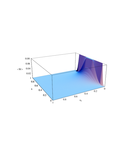
Figure 1: A three-dimensional view of the quantity $\sum_{a,\overline{a}}e_{a}^{2}x\,f_{1T}^{\perp(1)a}(x)\,H_{1}^{\perp(1)a}(z_{h})$, for scattering of unpolarized leptons on a polarized proton target, with production of $\pi^{+}$

We now have all the ingredients to calculate the weighted integrals proposed in Ref. [3]. Following the notations introduced therein, we will focus our attention on the following two of such objects.

$$\left<\frac{Q_{T}}{M}\;\sin(\phi^{l}_{h}-\phi^{l}_{S})\right>_{OTO}=$$ (13)

$$\frac{4\pi\alpha^{2}s}{Q^{4}}\,(1-y)\,\sum_{a,\overline{a}}e_{a}^{2}\ x\,f_{1T}^{\perp(1)a}(x)\,D_{1}^{a}(z_{h})\;.$$

A three-dimensional plot of the quantity
$\sum_{a,\overline{a}}e_{a}^{2}\ x\,f_{1T}^{\perp(1)a}(x)\,D_{1}^{a}(z_{h})$ is shown in Fig. 1. The shape of the surface as a function of $x$ and $z_{h}$ tells us that the effect due to the T-odd distribution function becomes sizeable for very small values of $z_{h}$ and intermediate values of $x$. It is clear that the effects due to the presence of the T-odd distribution function $f_{1T}^{\perp}(x)$ are small, but a suitably designed experiment may put limits on their size, or might establish their mere existence. This would be a crucial test for the presence of T-odd distribution functions and provide a deeper understanding of these phenomena.

 

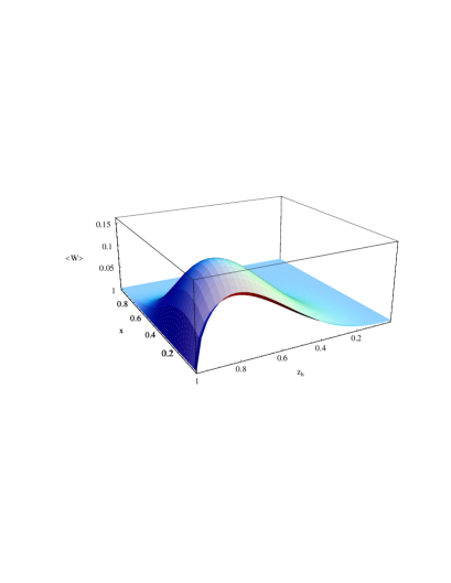
Figure 2: A three-dimensional view of the quantity $\sum_{a,\overline{a}}e_{a}^{2}\ x\,h_{1}^{a}(x)\,H_{1}^{\perp(1)a}(z_{h})$, for $OTO$ scattering with production of $\pi^{+}$.

If instead we choose the weight $W=(Q_{T}/M)\;\sin(\phi^{l}_{h}+\phi^{l}_{S})$, we obtain an object which is directly proportional to the T-odd fragmentation function $H_{1}^{\perp(1)}$ (see Table II, second line, in Ref. [3])

$$\left<\frac{Q_{T}}{M}\;\sin(\phi^{l}_{h}+\phi^{l}_{S})\right>_{OTO}=$$ (14)

$$\frac{4\pi\alpha^{2}s}{Q^{4}}\,(1-y)\,\sum_{a,\overline{a}}e_{a}^{2}\ x\,h_{1}^{a}(x)\,H_{1}^{\perp(1)a}(z_{h})\;.$$

As it clearly appears from the plot in Fig. 2, this time the shape of the quantity $\sum_{a,\overline{a}}e_{a}^{2}x\,h_{1}^{a}(x)\,H_{1}^{\perp(1)a}(z_{h})$ as a function of $x$ and $z_{h}$ is completely different from the previous one. It reaches its maximum for relatively small values of $x$ and for large values of $z_{h}$ and its overall size is at least a factor two bigger than the previous one. This means that a measure to reveal the effects of a non zero T-odd fragmentation function could easily be made at large values of $z_{h}$, where it is relatively easier to achieve larger statistics.

Finally, we give an evaluation of the ratios $H_{1}^{\perp a}/D_{1}^{a}$ and $f_{1T}^{\perp}/f_{1}$ (for $\pi^{+}$ production and considering only valence contributions). We find

$$\left|\frac{\int_{0.1}^{1}\,dz_{h}\ H_{1}^{\perp\mbox{\small fav}}(z_{h})}{\int_{0.1}^{1}\,dz_{h}\ D_{1}^{u/\pi^{+}}(z_{h})}\right|=0.076\;.$$ (15)

which gives a value of about $8\%$, in agreement with the result of Ref. [4]. For the T-odd distribution functions we have

$$\left|\frac{\int_{0.02}^{0.4}\,dx\,f_{1T}^{\perp\,u}(x)}{\int_{0.02}^{0.4}\,dx\,f_{1}^{u}(x)}\right|=0.083\;,$$ (16)

$$\left|\frac{\int_{0.02}^{0.4}\,dx\,f_{1T}^{\perp\,d}(x)}{\int_{0.02}^{0.4}\,dx\,f_{1}^{d}(x)}\right|=0.072\;,$$ (17)

which again gives an estimate of about 8%. We point out that the above estimates do not take into account the effects of evolution and that comparing integrated results neglects some kinematics factors.

Another example is the $\sin\phi$ single spin asymmetry, presented by the HERMES collaboration (see Avakian’s contribution in these proceedings), corresponding to:

$$\left<\frac{Q_{T}}{M}\;\sin(\phi^{l}_{h})\right>_{OLO}=\frac{4\pi\alpha^{2}s}{Q^{4}}\,(2-y)\,\sqrt{(}1-y)\,$$

$$\sum_{a,\overline{a}}e_{a}^{2}[xh_{1L}^{\perp(1)a}(x)\tilde{H}^{a}(z_{h})-x^{2}h_{L}^{a}(x)H_{1}^{\perp(1)a}(z_{h})].$$

We are now able to give some estimates of this quantity, under suitable approximations: our calculation will be presented in a forthcoming paper [14].

We acknowledge the support of the TMR program ERB FMRX-CT96-0008

References

• [1] R.L.Jaffe, X.Ji, Nucl. Phys. B375 (1992) 527.
• [2] M. Boglione, P.J. Mulders, hep-ph/9903354.
• [3] D. Boer and P.J. Mulders, Phys. Rev. D57, 5780 (1998).
• [4] A.V. Efremov et al., hep-ph/9812522.
• [5] M. Anselmino, M. Boglione and F. Murgia, Phys. Lett. B 362 (1995) 164.
• [6] M. Anselmino, A. Drago and F. Murgia, hep-ph/9703303.
• [7] J. Qiu and G. Sterman, Phys. Rev. Lett. 67 (1991) 2264, Nucl. Phys. B 378 (1992) 52; N. Hammon, O.V. Teryaev and A. ShΓ€fer, Phys. Lett. B 390 (1997) 409; D. Boer, P.J. Mulders and O.V. Teryaev, Phys. Rev. D57 (1998) 3057.
• [8] M. Anselmino, F. Murgia, Phys. Lett. B 442 (1998) 470.
• [9] M. Anselmino, M. Boglione, F. Murgia, hep-ph/9901442.
• [10] D.L. Adams et al, Phys. Lett. B261, 201 (1991) and Phys. Lett. B264, 462 (1991).
• [11] D.E. Soper, Phys. Rev. D 15 (1977) 1141; Phys. Rev. Lett. 43 (1979) 1847; J.C. Collins and D.E. Soper, Nucl. Phys. B194 (1982) 445; R.L. Jaffe, Nucl. Phys. B 229 (1983) 205.
• [12] J.D. Jackson, G.G. Ross, R.G. Roberts, Phys. Lett. B226 (1989) 159.
• [13] P. Abreu et al., Z.Phys. C73 (1996) 11-59
• [14] M. Boglione, P.J. Mulders, in progress.