Low $\mathbf{x}$ news for Monte Carlo
Eugene Levin ^a,

^a HEP Department, School of Physics, Tel Aviv University, Ramat Aviv, 69978, ISRAEL

Invited talk at Monte Carlo Workshop, DESY, 1999.

Abstract: This talk is a review of news in low $x$ physics which, I think, would be useful for writing of the Monte Carlo codes. The following topics are discussed here: (i) the next-to-leading order BFKLPomeron; (ii) two indications for shadowing corrections (SC) in DIS from HERA data; (iii) matching of “soft” and “hard” photon - proton interactions; and (iv) survival probability for large rapidity gap ( LRG ) processes in hadron-hadron scattering and DIS. I hope, that our current understanding of these topics will allow us to narrow the gap between the MC codes and our microscopic theory - QCD.

1 Introduction

Goals: The main goal of this talk is to share with you my understanding of the current situation in low $x$ physics looking at this subject from the angle of possible improvement of existing Monte Carlo codes. Everyone knows that the typical MC code for deep inelastic scattering ( DIS ) contains three parts: the perturbative QCD cascade, the hadronization stage and the matching between “soft” anf “hard” processes. Since we have no solid theoretical understanding of the hadronization stage and the “soft” processes, there is a danger to write a MC code that will describe the experimental data, but in which the clear connection with our microscopic theory - QCD, will be broken. This is the reason that MC experts should follow all theoretical and experimental news in implementing in MC everything that we have learned both theoretically and experimentally. My goal is to provide them with a guide to the recent achievements in low $x$ physics, which is a meeting point for all the complicated problems of perturbative and non-perturbative QCD.

Topics: The choice of the topics, that I would like to cover here, is dictated by my personal interests as well as by the considerable progress that has recently been made in their understanding. They are:

1. The next-to-leading order BFKL Pomeron;

2. Two indications for shadowing corrections (SC) in DIS from HERA data;

3. Matching of “soft” and “hard” photon - proton interactions;

4. Survival probability for large rapidity gap ( LRG ) processes in hadron-hadron scattering and DIS.

You can see that all above topics are closely related to our main problem- the matching between long distance ( non-perturbative ) physics and short distance ( perturbative ) approaches.

Sources of information: This talk is a report on what I learned at:

1. Theory Institute on Deep-Inelastic Diffraction - ANL, Sept.14 - 16,1998;

2. Workshop “Small $x$ and Diffraction Physics” - Fermilab, Sept. 17 - 20,1998;

3. 3-rd UK Phenomenology Workshop on HERA Physics - Durham, Sept. 21-25,1998;

4. During animated discussions with J. Bartels, M.Braun, W. Buchmüller, M. Ciafaloni, E. Gotsman, A. Kaidalov, Yu. Kovchegov, A. Kovner, J. Kwiecinski, L. Lipatov, U. Maor, A. Mueller, A. Martin, L. McLerran, D. Ross, M. Ryskin, G. Salam, M. Wüsthoff and many others, who shared with me their points of view on the topics that I am going to discuss;

5. My own thinking on the subject, which has only partly been reflected in the published papers.

2 The next-to-leading order BFKL Pomeron

Why do we love the BFKL Pomeron? I think, we can list here three main reasons for our love to the BFKL Pomeron:

1. The BFKL Pomeron [1] is a high energy asymptotic in a perturbative QCD approach which we call leading log (1/x ) approximation ( LL(x)A ). In the LL(x)A we select the diagrams using $\alpha_{S}\,\ll\,1$, $\alpha_{S}\,\ln Q^{2}\,\ll\,1$ but $\alpha_{S}\,\ln(1/x)\,\approx\,1$. The LL(x)A is quite different from the leading log ($Q^{2}$) approximation ( LL($Q^{2}$)A , $\alpha_{S}\,\ll\,1,\,\,\alpha_{S}\,\ln(1/x)\,\ll\,1,\,\,\alpha_{S}\,\ln Q^{2}\,\approx\,1$ ) in which the DGLAP evolution equations [2] were derived. We believe, that the BFKL Pomeron gives:

   1. A guide for the matching of perturbative QCD (pQCD) with non-perturbative one (npQCD), at least for high enegy scattering amplitude in DIS;

   2. A possibility to get the “soft” Pomeron contribution by taking into account the npQCD corrections in the BFKL Pomeron.

   We have several examples which support our hopes [3],[4].

2. The BFKL Pomeron is the only theoretical way to prove that at sufficiently high energy ( low $x$ ) the density of partons becomes large. In other words, the BFKL Pomeron shows that the mathching of the perturbative QCD parton cascade with the non-perurbative high energy asymptotics, goes through a new non-perturbative QCD stage i.e. a high parton density QCD ( see, for example, review [5] for details ). My personal opinion is that we do not need any theoretical arguments for a high parton density QCD, since the HERA experimental data show that the gluon density is high [6] [7]. However, the same experimental data we can be used as the experimental confirmation of the BFKL Pomeron;

3. The new HERA data shows that the BFKL Pomeron is needed to describe the forward jet production ( see Fig.1). These data change the entire attitude to the BFKL Pomeron, which from a theoretical toy, becomes a tool for the description of the experimental data and, therefore, a part of DIS phenomenology which should be included in the MC codes. The question still remains could the experimental data of Fig.1 be described without the BFKL Pomeron? You will answer this question better than me. However, Fig. 1 looks so impressive that it is difficult to believe that the agreement with the BFKL prediction is just a lucky coincidence.

   

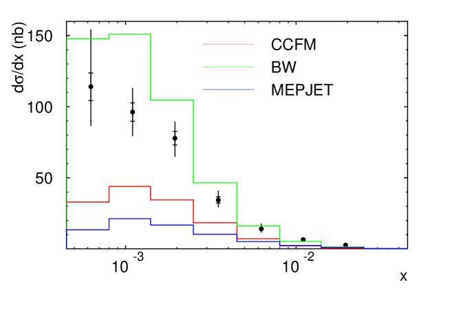
   Figure 1: The ZEUS’98 experimental data [8] for forward jet production and their description in MEPJET MC, in CCFM evolution equation [10] and in the BFKL approach ( BW )[9].

The map of disaster: It is well known that in the leading order the BFKL Pomeron leads to Regge-like asymptotics:

$$\sigma_{tot}(\,BFKL\,\,\,LO\,)\,\,\,\,\,\propto\,\,\,\,e^{\omega^{LO}_{L}\,(y-y_{0})\,\,-\,\,\frac{(r-r_{0})^{2}}{4D^{LO}(y-y_{0})}}\,\,,$$ (1)

where $y-y_{0}\,=\,\ln(s/s_{0})$ and $r-r_{o}\,=\,\ln(Q^{2}/Q^{2}_{0}$ ( see Fig.2-a for notations ).

This simple asymptotic in the leading order is based on:

1. The time structure of the parton cascade (see Fig. 2-b );

2. The separation between the longitudinal and transverse degrees of freedom;

3. The fact that gluon emission leads to $\sigma\,\,\propto\,\,\frac{1}{x^{\omega_{L}}}$;

4. The diffusion in log of transverse momenta.

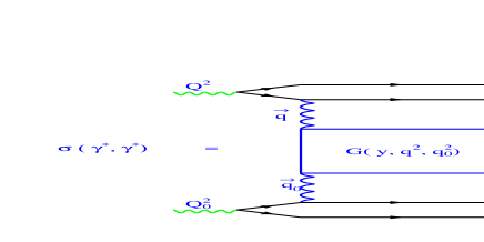
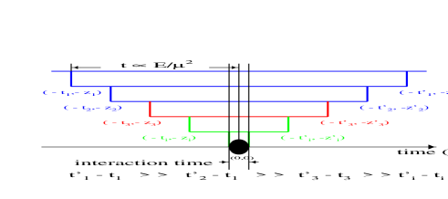
Figure 2-a	Figure 2-b

Figure 2: $\gamma^{*}\gamma^{*}$ - interaction in the BFKL approach ( a ) and the time structure of the BFKL Pomeron ( b ).

Recently, the next-to-leading order corrections to the kernel of the BFKL equation has been calculated [11] [12] and it turns out that these corrections are so large that they could change the entire understanding of the structure of the parton cascade in pQCD. Indeed, in the NLO:

• $\omega_{L}\,\,<\,\,0$ at $q^{2}_{0}\,\mathrel{\hbox to0.0pt{\lower 4.0pt\hbox{\hskip 1.0pt$\sim$}\hss}\raise 1.0pt\hbox{$<$}}\,30\,GeV^{2}$ [11][12][13] ( see Fig.2-a ). It means that in a large kinematic region, the BFKL emission is suppressed, and only the Born term contributes;

• For $q^{2}_{0}\,\mathrel{\hbox to0.0pt{\lower 4.0pt\hbox{\hskip 1.0pt$\sim$}\hss}\raise 1.0pt\hbox{$<$}}\,3\,10^{6}\,GeV^{2}$ $D\,<\,0$ [14]. It means that there is no diffusion in log of transverse momenta in the NLO BFKL. It also turns out that $D\,<\,0$ leads to oscillation of the total cross section [14] [3] which shows that the NLO BFKL has a serious pathology;

• In the NLO, the Regge-like asymptotics of Eq.(  1 ) is valid only in the limited range of energy $y-y_{0}=\ln(s/qq_{0})\,\leq\,(\alpha_{S})^{-\frac{5}{3}}$ [3] [16]. For large values of $y-y_{0}$ an extra term appears in exponent of Eq.( 1 ) which is proportional to $\alpha_{s}^{5}\,(y-y_{0})^{3}$ [16] [3]. Therefore, we cannot hope that in NLO BFKL we will get Regge-like asymptotics [16] [3][17].

Even a slight glance at the difficulties, listed above, shows that the main properties of the LO BFKL are broken in the NLO.

A possible way out - the main idea of resummation: The BFKL equation in the NLO can be written in the form:

$$\frac{\partial G(y,\vec{q},\vec{q}_{0})}{\partial y}\,\,=\,\,\delta^{(2)}(\vec{q}-\vec{q}_{0})\,\,+\,\,\int\,d^{2}q^{\prime}\,K(\vec{q},\vec{q}^{\prime})\,G(y,\vec{q}^{\prime},\vec{q}_{0})\,\,,$$ (2)

where the NLO kernel $K(\vec{q},\vec{q}^{\prime})$ can be written as

$$K(\vec{q},\vec{q}^{\prime})\,\,=\,\,\alpha_{S}(q^{2})\,\,\{\,\,K^{LO}(\vec{q},\vec{q}^{\prime})\,\,+\,\,K^{NLO}(\vec{q},\vec{q}^{\prime})\,\,\}\,\,=$$ (3)

$$\,\,\frac{r_{0}}{r}\,K_{conf}(\vec{q},\vec{q}^{\prime})\,\,=\,\,\frac{r_{0}}{r}\,\{\,\alpha_{S}(q_{0})\,K^{LO}\,\,+\,\,\alpha^{2}_{S}(q_{0})\,K^{NLO}\,\}\,\,.$$

In Ref. [11] it was found that the largest contributions to $K^{NLO}$ with the Fadin-Lipatov choice of the energy variable $y-y_{0}\,=\,\ln(s/qq_{0})$ is $K^{NLO}\,\,\propto\,\,\alpha^{2}_{S}\,\,\ln^{2}(q^{2}/q^{\prime 2})$. One can see that such a term appears as a change of the energy scale in the normal double log contribution. Indeed, term $\alpha^{2}_{S}\,\ln(q^{2}/q^{2}_{0})\,\ln^{2}(s/q\,q_{0})$ leads to $\alpha^{2}_{S}\,\ln^{2}(q^{2}/q^{\prime 2})\,\ln(s/q^{2}_{0})$ -contribution if we cange the energy scale from $s_{0}=q\,q_{0}$ to $s_{0}=q^{2}_{0}$.

The above example shows that in the NLO we lost the very important property of the LO BFKL Pomeron, namely, matching the BFKL approach with the DGLAP one, for both $q^{2}\,\,\gg\,\,q^{2}_{0}$ and $q^{2}_{0}\,\,\gg\,\,q^{2}$. The main idea , suggested by G.Salam [18] and by M.Ciafaloni [19], is to replace the NLO kernel of the BFKL equation by the new kernel in which subleading $\alpha^{n}_{S}$ - corrections to the BFKL equation have been resummed in a such way that

$$K^{BFKL}_{resummed}\,\,\,\,\longrightarrow\,\,\,\,K^{DGLAP}\,\,,$$ (4)

for $q^{2}\,\,\gg\,\,q^{2}_{0}$ and for $q^{2}_{0}\,\,\gg\,\,q^{2}$.

A possible way out - a toy model: Actually, the influence of the energy scale on the BFKL equation has been studied by Andersson,Gustafson and Samuelson [20] in their Linked Dipole Chain Model which reproduces the DGLAP double logs $\ln(1/x)\,\ln(q^{2}/q^{2}_{0})$ for $q^{2}\,\,\gg\,\,q^{2}_{0}$ and for $q^{2}_{0}\,\,\gg\,\,q^{2}$.

The key equation of this model

$$\frac{\partial G(y,\vec{q},\vec{q}_{0})}{\partial y}\,\,=\,\,\frac{\alpha_{S}N_{c}}{\pi}\,\,\int\,\frac{d^{2}l}{\pi\,l^{2}}\,\,\{\,\,G(x^{\prime},q^{\prime 2})\,\,-\,\,G(x^{\prime},q^{2})\,\Theta(q-l)\,\,\}$$ (5)

with $\vec{l}\,\,=\,\vec{q}\,\,-\,\,\vec{q}^{\prime}$ and

$$y\,=\,\ln(1/x)\,\,;\,\,\,\,\,\,\,x\,=\,\frac{q^{2}}{s}\,\,;\,\,\,\,\,x^{\prime}\,\,=\,\,{\rm max}(x,x\,\frac{q^{\prime 2}}{q^{2}})\,\,.$$

This equation is the BFKL one if $x^{\prime}=x$. With a new definition of the energy variable $x^{\prime}$, the equation sums some of the next-to-leading order corrections to the BFKL kernel.

Fig.3-a shows the Mellin image of the kernel for the BFKL case ( $x=x^{\prime}$ , $\chi^{(0)}$ ), for the next-to-leading order correction to the BFKL equation ( $\chi^{(0+1)}$) and for the kernel of Eq.( 5 ) ( all orders). One can see, that the NLO gives a minimum at $\nu$ = 0 which corresponds to oscillation in the total cross section. However, the resummed kernel (all orders) has the same qualitatively behaviour as the LO BFKL kernel. In Fig.3-b the BFKL intercept is plotted for the solution of Eq.( 5 ). One can see that the negative intercept for $\alpha_{S}\,\,>$ 0.2 in the NLO is irrelevant for the intercept of Eq.( 5 ), which is about twice smaller than the intercept of the LO BFKL equation, but is definately positive.

Figure 3-a	Figure 3-b

Figure 3: The Mellin image of the toy kernel ( a) and the intercept of the toy-Pomeron (b ). See text for detail description.

Therefore, we can conclude from this toy model that the principle, formulated in the previous subsection ( see Eq.(  4) ), works and the resummation has a chance to heal our difficulties in the NLO BFKL equation.

A possible way out - an example of resummation:

G.Salam [18], using the principle of Eq.(  4 ), suggested how to deal with unphysical logs of $\alpha^{2}_{S}\,\ln^{2}(q^{2}/q^{2}_{0})$ - type. He demonstrated how to extend ( resum ) the NLO BFKL kernel so as to guarantee the concellation of unphysical logs to all orders and to provide the matching of the BFKL Pomeron with the DGLAP evolution equation. Unfortunately, the prescription for resummation is ambiguous and Salam suggested four realizations ( schemes) of his ideas. It should be mentioned that other schemes were advocated [12] as well as the arguments for Salam’s schemes 3 and 4 were suggested [12][21] [22][23]. In Refs. [21] [22] the criteria was suggested following the idea of Lipatov: the independence of the resummed result on the energy cutoff. This criteria is in the same spirit as the independence of the result on the factorization scale and it can be a good first step in understanding of the accuracy of the resummed BFKL Pomeron.

Fig.4 shows the behaviour of the BFKL intercept ( $\omega_{L}=\bar{\alpha}_{S}\,\chi(\frac{1}{2}))$ in Eq.( 1 )) and the width of the BFKL Pomeron ( $D=\bar{\alpha}_{S}\,\chi^{\prime\prime}(\frac{1}{2})$ ). One can see that the BFKL Pomeron intercept is positive in contrast with the NLO approximation. $D$ is also positive, but only for schemes 3 and 4. The second important conclusions that we can derive from Fig.4, is the similarity of the resummed NLO BFKL kernel with the toy model which has been discussed.

Figure 4: The BFKL Pomeron intercept ($\omega_{L}\,=\,\bar{\alpha}_{S}\,\chi(\frac{1}{2})$ and the width of the BFKL Pomeron ( $D\,=\,\bar{\alpha}_{S}\,\chi^{\prime\prime}(\frac{1}{2})$).

Resume and recommendations: Let me share with you to-day ( 20.04.1999 ) my understanding of the BFKL Pomeron standing.

1. Large NLO corrections to the BFKL kernel left us without any theoretical predictions for both the BFKL Pomeron intercept ( $\omega_{L}$ in Eq.( 1 ) ) and the BFKL Pomeron width ( $D$ in Eq.( 1 ) ). We can introduce both of them as phenomenological parameters in a MC code,, which should be extracted from the experimental data. The resummed BFKL kernel can be used to check how reasonable these extracted values of $\omega_{L}$ and $D$ will be;

2. For the running QCD coupling constant ($\alpha_{S}$ ) the Regge-like asymptotic of Eq.( 1 ) can be justified only in a limited range of energies. Therefore, it is better to use the numerical solution of the BFKL equation than the analytical expression of Eq.( 1 );

3. The main qualitative properties of the parton BFKL cascade remain the same as in LO BFKL, for the NLO resummed BFKL equations. This is the very important conclusion for MC, which is the most striking theoretical result;

4. It is better to use the Linked Dipole Chain ( LDC ) Monte Carlo [24] than the BFKL equation itself. However, we first need to check that the LDC MC describes the LDC model [20].

3 Two indications for shadowing corrections from HERA data

HERA puzzle: The wide spread opinion is that HERA experimental data for $Q^{2}\,\mathrel{\hbox to0.0pt{\lower 4.0pt\hbox{\hskip 1.0pt$\sim$}\hss}\raise 1.0pt\hbox{$>$}}\,1\,GeV^{2}$ can be described using only the DGLAP evolution equations, without any other ingredients such as shadowing corrections, high twist contributions and so on ( see, for example reviews [6] [7] ). On the other hand, the most important HERA discovery is the fact that the density of gluons ( gluon structure function ) becomes large in HERA kinematic region ( see Fig.5 ).

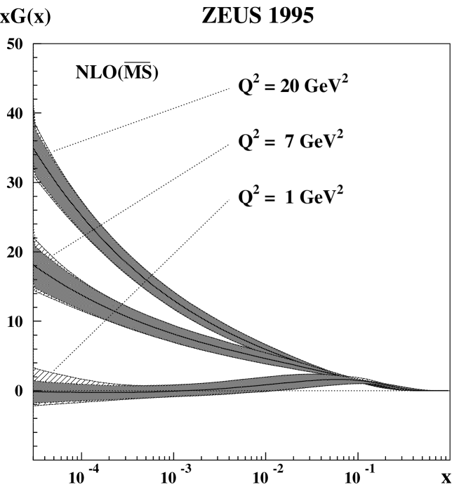
Figure 5: ZEUS [25] data for gluon structure function ($xG(x,Q^{2})$.

The value of the gluon density turns out to be so large that parameter

$$\kappa\,\,\,=\,\,\,\frac{3\,\pi^{2}\alpha_{S}}{2Q^{2}}\,\times\,\frac{xG(x,Q^{2})}{\pi\,R^{2}}\,\,,$$ (6)

which determines the value of SC [26] [27] [74] [29], reaches unity

$$\kappa\,=\,\frac{3\,\pi^{2}\alpha_{S}}{2Q^{2}_{0}(x)}\,\times\,\frac{xG(x,Q^{2}_{0}(x))}{\pi\,R^{2}}\,\,=\,\,1$$ (7)

in HERA kinematic region (see Fig.6 )

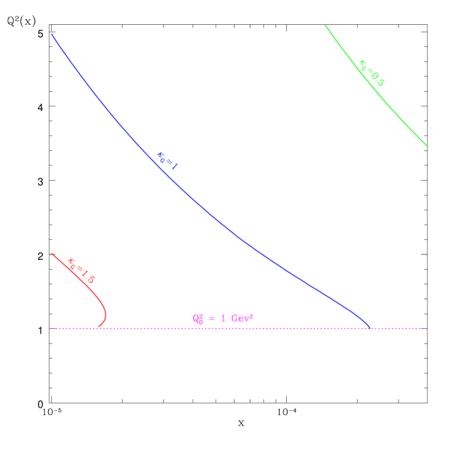
Figure 6: Kinematic plot with lines $\kappa$ = 0.5, 1 and 1.5 .

It means that in large kinematic region where $\kappa\,\mathrel{\hbox to0.0pt{\lower 4.0pt\hbox{\hskip 1.0pt$\sim$}\hss}\raise 1.0pt\hbox{$>$}}\,1$ ( to the left from line $\kappa\,=\,1$ in Fig.6 ), we expect that the SC should be large and important for the description of the experimental data. At first sight such expectations are in clear contradiction with the experimental data. Certainly, this fact gave rise to the suspicion ( or even mistrust ) that our theoretical approach to the SC is not consistent. However, the revision and re-analysis of the SC have been completed [30] [31] [32] [33] [34][29] with the result that $\kappa$ is the parameter which is reponsible for the value of SC.

Therefore, we face a puzzling question: where are SC in DIS?  I am happy to tell you that we now where is the energy have two indications in the HERA experimental data that the SC are rather large and important. These indications are:

1. $x_{P}$ - behaviour of the cross section of the diffractive dissociation ( $\sigma_{DD}$ ) in DIS;

2. $Q^{2}$ - behaviour of $F_{2}$-slope ( $\frac{\partial F_{2}(x_{B},Q^{2})}{\partial\ln Q^{2}}$   ).

Here, we would like to discuss both phenomena and their relation to the SC.

3.1 $\mathbf{x_{P}}$ - dependence of $\mathbf{\sigma_{DD}}$

Data: Both collaborations ( H1 and ZEUS ) found that

$$\sigma_{DD}\,\,\,\propto\,\,\,\frac{1}{x^{2\,\Delta_{P}}}$$ (8)

where $\Delta_{P}$  = $\alpha_{P}(0)\,\,-\,\,1$. The values of $\alpha_{P}(0)$ are:

$\mathbf{\bullet}$    H1 [35] :	$\alpha_{P}(0)$ = 1.2003  $\pm$ 0.020 (stat.) $\pm$  0.013 (sys.)  ;
$\mathbf{\bullet}$    ZEUS[36] :	$\alpha_{P}(0)$  =  1.127  $\pm$    0.009 (stat.)   $\pm$   0.012 (sys.)  .

In Fig.7 the ZEUS data on the Pomeron intercept are plotted together with the intercept the “soft” Pomeron [37]. It is clear that the Pomeron intercept for the diffractive processes in DIS is higher than the intercept of the “soft” Pomeron.

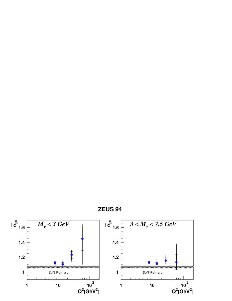
Figure 7: ZEUS[36] data on the Pomeron intercept for $\sigma_{DD}$ in DIS.

Why is it surprising and interesting? To answer this question let us consider the simplest diffractive process - the diffractive production of the quark - anti quark pair with mass $M$ ( see Fig.8 )

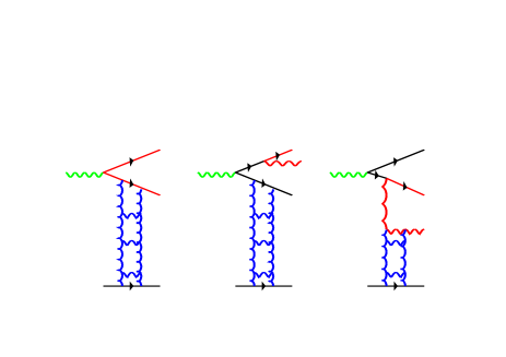
Figure 8-a	Figure 8-b

Figure 8: The simplest examples of the diffractive processes: ( a ) the production of quark - antiquark pair with mass $M$ and (b) the production of quark - antiquark pair with one extra gluon.

As it was shown ( see Refs. [38] [39] [40] ) the cross sections of this process are proportional to:

$$x_{P}\,\frac{d\sigma^{T}_{DD}(\gamma^{*}\,\rightarrow\,q+\bar{q})}{dx_{P}dt}\,\,\,\propto\,\,\,\int^{\frac{M^{2}}{4}}_{Q^{2}_{0}}\,\,\frac{dk^{2}_{\perp}}{k^{2}_{\perp}}\,\,\times\,\,\frac{\left(\,\alpha_{S}\,\,x_{P}\,G(x_{P},\frac{k^{2}_{\perp}}{1-\beta})\,\right)^{2}}{k^{2}_{\perp}}\,\,$$ (9)

for transverse polarized virtual photon and

$$x_{P}\,\frac{d\sigma^{L}_{DD}(\gamma^{*}\,\rightarrow\,q+\bar{q})}{dx_{P}dt}\,\,\,\propto\,\,\,\int^{\frac{M^{2}}{4}}_{Q^{2}_{0}}\,\,\frac{dk^{2}_{\perp}}{Q^{2}}\,\,\times\,\,\frac{\left(\,\alpha_{S}\,\,x_{P}\,G(x_{P},\frac{k^{2}_{\perp}}{1-\beta})\,\right)^{2}}{k^{2}_{\perp}}$$ (10)

for the longitudinal polarized photon. In these formulae we used the notation ( see Fig.8 ): $Q^{2}$ is the photon virtuality; $M$ is the produced mass; $x_{P}\,\,=\,\,\frac{Q^{2}+M^{2}}{s}$ , where $s$ is the energy of virtual photon proton collisions; and $\beta\,=\,\frac{Q^{2}}{Q^{2}\,+\,M^{2}}$.

The same factor also enters a more complicated process as, for example, a diffractive production of the quark - antiquark pair and one extra gluon (see Fig.8-b ). Indeed, the cross section of this process is proportional to [40]:

$$x_{P}\,\frac{d\sigma^{T}_{DD}(\gamma^{*}\,\rightarrow\,q\,+\,\bar{q}\,+\,G)}{dx_{P}dt}\,\,\,\propto\,\,\,\,\int^{\frac{M^{2}}{4}}_{Q^{2}_{0}}\,\,\frac{dk^{2}_{\perp}}{k^{2}_{\perp}}\,\,\times\,\ln(M^{2}/4k^{2}_{\perp})\,\,\times\,\,\frac{\left(\,\alpha_{S}\,\,x_{P}\,G(x_{P},k^{2}_{\perp})\,\right)^{2}}{k^{2}_{\perp}}\,\,.$$ (11)

One can see that for the transverse polarized photon the diffractive cross section stems from the low values of the transverse momenta $k_{\perp}$ ( see Eq.( 9 ) and Eq.( 11 ) ) if we use for $xG$ the solution of the DGLAP equations. However, the situation changes crucially if we take into account the SC in expression for $xG$. For estimates of the value of the SC, we use the Glauber - Mueller approach [74] for $xG$, namely [40] [41]:

$$x_{P}G^{SC}(x_{P},k^{2}_{\perp})\,\,\,=\,\,\,\frac{2}{\pi^{2}}\,\int^{1}_{x_{P}}\,\frac{dx^{\prime}}{x^{\prime}}\int^{\infty}_{\frac{1}{k^{2}_{\perp}}}\,\,\frac{dr^{2}}{r^{4}}\int db^{2}_{t}\{\,\,1\,\,\,-\,\,\,e^{-\kappa^{DGLAP}(x^{\prime},r^{2})\,S(b_{t})}\,\,\}\,\,$$ (12)

where $S(b_{t})\,\,=\,\,e^{-\frac{b^{2}_{t}}{R^{2}}}$.

From Eq.( 12 ) we can see that in the limit of low $x$

$$x_{P}G(x_{P},k^{2}_{\perp})\,\,\,\,\,\Longrightarrow\,\,\,\,k^{2}_{\perp}\,R^{2}\,\,\int^{1}_{x}\,\frac{dx^{\prime}}{x^{\prime}}\,\ln\kappa(x^{\prime},\frac{1}{k^{2}_{\perp}})$$ (13)

if $k^{2}_{\perp}\,\,\ll\,\,Q^{2}_{0}(x)$, where $Q^{2}_{0}(x)$ is plotted in Fig.6. Therefore, the substitution of $xG^{SC}$ in Eq.( 9 ) and Eq.( 11 ) leads to the situation that the integral over $k^{2}_{\perp}$ is not infrared divergent, and the main contribution comes from the region of $k^{2}_{\perp}$ of the order of $Q^{2}_{0}(x_{P})$. It means that

$$x_{P}\,\frac{d\sigma_{DD}}{dx_{P}dt}\,\,\,\,\,\Longrightarrow\,\,\,\,\,\frac{1}{Q^{2}_{0}(x_{P})}\,\,\times\,\,\left(\,x_{P}\,G(x_{P},Q^{2}_{0}(x_{P}))\,\right)^{2}\,\,\,\,\propto\,\,\,\frac{1}{x^{2\lambda_{eff}(Q^{2})}_{P}}$$ (14)

Eq.( 14 ) allows us to find the typical distances which are reponsible for the diffraction dissociation in DIS. Comparing the experimental values of $\lambda_{eff}(Q^{2})$ with the ones calculated using Eq.( 12 ) (see Fig.9 ) , one can conclude that the typical $k^{2}_{\perp}$ is not small, but rather $k^{2}_{\perp}\,\,\approx\,\,1-2\,GeV^{2}$ [40][41],, if we take $x_{P}\,\approx\,10^{-3}$, or even larger.

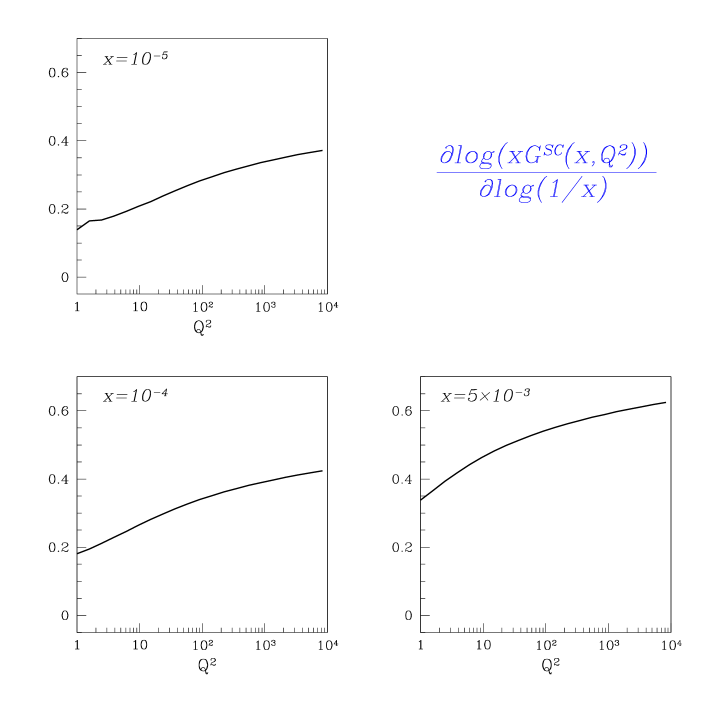
Figure 9: $\lambda(Q^{2})\,=\,\frac{1}{x_{P}\,G^{SC}(x_{P},k^{2}_{\perp})}\,\,\frac{dx_{P}\,G^{SC}(x_{P},k^{2}_{\perp})}{d\ln(1/x_{P})}$ calculated using Eq.( 12 ).

It should be stressed that the diffraction dissociation for longitudinally polarized photon ( see Eq. 10 ) for quark - anriquark production comes from long distances and its cross section is proportional to

$$x_{P}\,\frac{d\sigma^{L}_{DD}(\gamma^{*}\,\rightarrow\,q+\bar{q})}{dx_{P}dt}\,\,\,\propto\,\left(\,\alpha_{S}\,x_{P}\,G(x_{P},\frac{M^{2}}{4(1-\beta)})\,\right)^{2}$$ (15)

One of the striking feature of the experimental data, is the fact that the cross section of the diffractive dissociation in DIS and the total DIS cross section have the same energy dependence. Recently, an explanation of such a behaviour was suggested based on the SC contributions[42] [43] [44]. Indeed, the total cross section and cross section of diffractive production are equal to:

$$\sigma_{tot}(\gamma^{*}p)\,\,\,=\,\,\,\int d^{2}r_{t}\int^{1}_{0}\,dz\,\,|\Psi(Q^{2};r_{t},z)|^{2}\,\,\,\sigma_{tot}(r^{2}_{t},x)\,\,;$$ (16)

$$\sigma_{DD}(\gamma^{*}p)\,\,\,=\,\,\,\int d^{2}r_{t}\int^{1}_{0}\,dz\,\,|\Psi(Q^{2};r_{t},z)|^{2}\,\,\,\{\,\sigma_{tot}(r^{2}_{t},x)\,\,-\,\,\sigma_{in}(r^{2}_{t},x)\,\}\,\,;$$ (17)

where $\sigma_{tot}(r^{2}_{r},x)$ and $\sigma_{DD}(r^{2}_{r},x)$ are total and inelastic cross section for dipole with distance $r_{t}$ between quark and antiquark, respectively.

The solution of the unitarity constraint for dipole scattering gives:

$$\sigma_{tot}(r^{2}_{t},x)\,\,=\,\,2\,\int\,d^{2}b_{t}\,\{\,1\,\,\,-\,\,\,e^{-\kappa^{DGLAP}_{q}\,S(b_{t})}\,\}\,\,;$$ (18)

$$\sigma_{in}(r^{2}_{t},x)\,\,=\,\,\,\int\,d^{2}b_{t}\,\{\,1\,\,\,-\,\,\,e^{-2\,\kappa^{DGLAP}_{q}\,S(b_{t})}\,\}\,\,;$$ (19)

where $k^{DGLAP}_{q}\,\,=\frac{4}{9}\,\,\kappa^{DGLAP}$ ( see Eq.( 6 ) ).

After integration over $z$ we get for transverse polarized photon [46]

$$\int^{1}_{0}\,dz\,\,|\Psi_{T}(Q^{2};r_{t},z)|^{2}\,\,\,=\,\,\,\frac{4\,\alpha_{em}N_{c}}{3\,\pi^{2}\,Q^{2}}\,\times\,\frac{1}{r^{4}_{t}}\,\,.$$ (20)

Using the expilict expression for $S(b_{t})$ and assuming that the anomalous dimension of $xG$ is not large $\gamma\,\ll\,1$ ( in this case we can replace $xG(x,k^{2}_{t})$ by $xG(x,Q^{2})$ in the integrals ) we can obtain [44]:

$$\sigma_{tot}(\gamma^{*}p)\,\,\,\propto\,\,2\,R^{2}\,\{\,\ln(\kappa_{q})\,\,+\,\,C\,\,(\,1\,+\,\kappa_{q}\,)\,E_{1}(\kappa_{q})\,+\,1\,-\,e^{-\kappa_{q}}\,\}\,\,;$$ (21)

$$\sigma_{DD}(\gamma^{*}p)\,\,\,\propto\,\,\,2\,R^{2}\,\{\,\ln(\kappa_{q})\,\,+\,\,C\,\,(\,1\,+\,\kappa_{q}\,)\,E_{1}(\kappa_{q})\,+\,1\,-\,e^{-\kappa_{q}}\,\}\,\,$$ (22)

$$-\,\,\,R^{2}\,\{\,\ln(2\,\kappa_{q})\,\,+\,\,C\,\,(\,1\,+\,2\,\kappa_{q}\,)\,E_{1}(2\,\kappa_{q})\,+\,1\,-\,e^{-2\,\kappa_{q}}\,\}\,\,;$$

where $C$ is the Euler constant and $E_{1}$ is the interral exponant [45].

These formulae indicate that $\sigma_{tot}\,\rightarrow xG(x,Q^{2})$ and $\sigma_{DD}\,\rightarrow\,\left(\,xG(x,Q^{2})\,\right)^{2}$ for small $\kappa_{q}\,\ll\,1$, but at $\kappa_{q}\,\,\gg\,\,1$ we obtain that

$$\sigma_{tot}(\gamma^{*}p)\,\,\,\longrightarrow\,\,2\,R^{2}\,\{\ln(\kappa_{q})\,\,+\,\,C\,\}\,\,;$$ (23)

$$\sigma_{DD}(\gamma^{*}p)\,\,\,\longrightarrow\,\,\,2\,R^{2}\,\{\,\ln(\kappa_{q})\,\,+\,\,C\,\}\,\,-\,\,R^{2}\,\{\,\ln(2\,\kappa_{q})\,\,+\,\,C\,\}\,\,=\,\,R^{2}\,\ln(\kappa_{q})\,\,=\,\,\frac{1}{2}\,\sigma_{tot}.$$ (24)

This simple calculation shows that indeed at low $x$, where $\kappa_{q}$ is expected to be large, $\sigma_{DD}$ and $\sigma_{tot}$ [44], should have the same energy dependence but accuracy of such a statement is controlled by ratio $C/ln(\kappa_{q})\,\,\ll\,\,1$. In Refs. [42] and [43] one can find estimates of how SC reveal themselves in real experimental situation. It turns out that they are able to describe the experimental energy behaviour of $\sigma_{DD}$.

3.2 The effect of screening on $\mathbf{Q^{2}}$ - dependence of the $\mathbf{F_{2}}$ - slope.

Data: The experimental data [47] for the $F_{2}$ - slope $\frac{dF_{2}(x,Q^{2})}{d\ln Q^{2}}$ is shown in Fig.10 ( Caldwell plot ). These data give rise to a hope that the matching between “hard” ( short distance ) and “soft” (long distance ) processes occurs at sufficiently large $Q^{2}$. Indeed, the $F_{2}$ - slope starts to deviate from the DGLAP predictions around $Q^{2}\,\approx\,5-8\,GeV^{2}$.

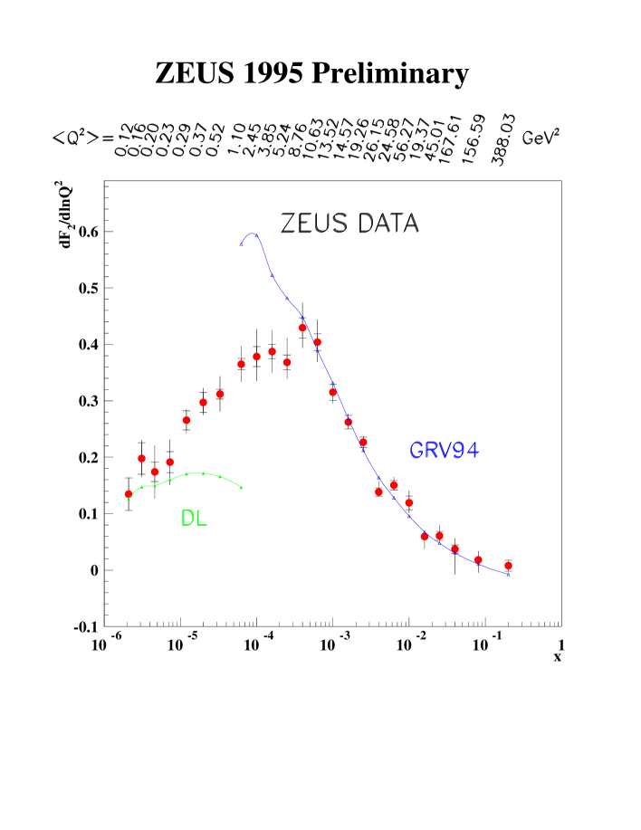
Figure 10: The ZEUS data on the $F_{2}$ - slope ( Caldwell plot ).

Such a large value of this separation parameter between short and long distance processes leads to a natural question:“Could the experimental behaviour of the $F_{2}$ - slope as a function of $Q^{2}$ be a manifestation of the shadowing corrections or, better to say, of the saturation of the gluon density in DIS ?”. The answer [48] [49] [41] is: “Yes”.

$\mathbf{F_{2}}$ - slope and SC: In Refs. [49] [41] the influence of the SC on the behaviour was calculated using Eq.( 12 ) and similar formula in quark-antiquark sector. The result is given in Fig.11 where the $F_{2}$ - slope in ALLM parameterization [50] is also plotted. Comparison with the experimental data as well as with the ALLM predictions shows that the SC can give a plausible explanation of the effect.

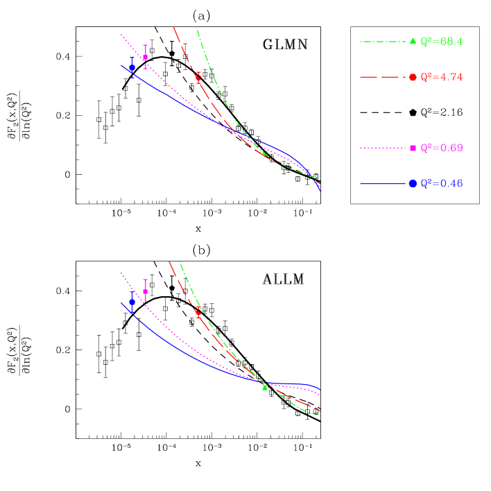
Figure 11: The $F_{2}$ - slope in QCD calculations taking into account SC ( GLMN ) [41] and in ALLM’97 parameterization [50], which describes the matching between “soft ” and “hard” interactions in DIS.

We would like to draw your attention to the fact that at fixed value of $Q^{2}$ the SC do not lead to qualitative change of $x$ - dependence of the $F_{2}$-slope ( see lines with fixed $Q^{2}$ in Fig.11 ). However, the saturation of the gluon density gives $F_{2}\,\,\propto\,\,Q^{2}\,R^{2}$ at $Q^{2}\,<\,Q^{2}_{0}(x)$. Therefore, the $F_{2}$ - slope shows a decrease at small $Q^{2}$. The calculations support the idea that the experimmental selection of the data on the $F_{2}$ - slope shows predicted $Q^{2}$-dependence. However, it is important to stress that only data on $F_{2}$ - slope at fixed energy ( or $x$ ) would clarify how much of the experimentally observed effect is related to the $Q^{2}$ - dependence. It is worthwhile mentioning that the ALLM’97 parameterization which describes phenomenologically the matching between “hard” and “soft” interactions in DIS, predicts the same behaviour of the $F_{2}$ - slope as the SC calculations ( see Fig.11 ).

3.3 Why these two facts are still only the indications of SC contributions?

I hope that I have convinced you that the SC provide a natural explanation of both experimental effects. Even more, the new experimental data give a possible way to understand and resolve the HERA puzzle, that has been formulated at the beginning of this section. We have expected such effects for a long time, and the SC recieved strong support from the experiment.

However, we cannot not make a final conclusion because both the experimental sets of data on $x_{P}$-dependence of the diffractive cross section, and on $Q^{2}$ - dependence of the $F_{2}$ - slope can have an alternative explanation. For example, the MRST parameterization [51] gives the explanation for the $F_{2}$ - slope behaviour assuming the strange behaviour of the gluon structure function at the initial virtuality $Q^{2}=Q^{2}_{0}$ - decreasing at low $x$.

Nevertheless, we would like to stress that the SC give a good agreement with the ALLM’97 parametrization in the wide range of $Q^{2}$ and $x$. This provides strong support for SC which, we hope, will be confirmed by the future experimental data.

We need to introduce SC in the Monte Carlo codes to be prepared for the future experiments.

4 Matching of “soft” and “hard” photon - proton interactions

Gribov’s approach: The rich and high precision data on deep inelastic $ep$ scattering at HERA [52] [53], covering both low and high $Q^{2}$ regions, lead to a theoretical problem of matching the non-perturbative (“soft”) and perturbative (“hard ”) QCD domains. This challenging problem has been under close investigation over the past two decades, starting from the pioneering paper of Gribov [54] ( see also [55] ).

Gribov suggested two stages of the $\gamma^{*}p$ interaction in any QCD description (see Fig.12-a):

1. The $\gamma^{*}$ converts into a hadron system (quark-antiquark pair to lowest order) well before the interaction with the target;

2. The quark-antiquark pair (or hadron system) then interacts with the target.

These two stages are expressed explicitly in the double dispersion relation suggested in Ref. [54] ( see Fig.12-b ):

Figure 12-a	Figure 12-b

Figure 12: Gribov’s approach to photon - hadron interaction: (a) the time structure of this interaction and (b) the double mass dispertion relation.

$$\sigma(\gamma^{*}N)=\frac{\alpha_{em}}{3\pi}\int\frac{\Gamma(M^{2})dM^{2}}{(Q^{2}+M^{2})}\sigma(M^{2},M^{\prime 2},s)\frac{\Gamma(M^{\prime 2})dM^{\prime 2}}{(Q^{2}+M^{\prime 2})},$$ (25)

where $M$ and $M^{\prime}$ are the invariant masses of the incoming and outgoing quark-antiquark pairs, $\sigma(M^{2},M^{\prime 2},s)$ is the cross section of a $q\bar{q}$ interaction with the target, and the vertices $\Gamma^{2}(M^{2})$ and $\Gamma^{2}(M^{\prime 2})$ are given by $\Gamma^{2}(M^{2})=R(M^{2})$, where $R(M^{2})$ is the ratio:

$$R(M^{2})=\frac{\sigma(e^{+}e^{-}\to\mbox{hadrons})}{\sigma(e^{+}e^{-}\to\mu^{+}\mu^{-})},$$ (26)

which has beem measured experimentally.

The key problem in all approaches utilizing Eq.( 25 ) is the description of the cross section $\sigma(M^{2},M^{\prime 2},s)$.

1. We introduce $M_{0}\,\,\approx\,\,1\,GeV$ in the integrals over $M$ and $M^{\prime}$, which play the role of a separation parameter. For $M,\,M^{\prime}\,>\,M_{0}$ the quark - antiquark pair are produced at short distances ( $r_{\perp}\,\,\propto\,\frac{1}{M}\,\,<\,\,\frac{1}{M_{0}}$ ), while for $M,\,M^{\prime}\,<\,M_{0}$ the distance between quark and antiquark is too long ($r_{\perp}\,\,\propto\,\frac{1}{M}\,\,>\,\,\frac{1}{M_{0}}$), and we cannot treat this $q\bar{q}$ - pair in pQCD. Actually, we cannot even describe the produced hadron state as a $q\bar{q}$ - pair;

2. For $M,\,M^{\prime}\,<\,M_{0}$ we use the Additive Quark Model [56] in which

   $$\sigma(M^{2},M^{\prime 2},s) = \sigma^{soft}_{N}(M^{2},s)\,\delta(M^{2}\,-\,M^{\prime 2})$$ (27)

   $$= \left(\,\sigma_{tot}(qN)\,+\,\sigma_{tot}(\bar{q}N)\,\right)\,\delta(M^{2}\,-\,M^{\prime 2})$$

3. For $M,\,M^{\prime}\,>\,M_{0}$ we consider the system with mass $M$ and/or $M^{\prime}$ as a short distance quark - antiquark pair, and describe its interaction with the target in pQCD. The exact formulae for $\sigma^{hard}(M^{2},M^{\prime 2},s)$ is given in Ref. [57]), but the key property of these formulae that this interaction can be expressed through the gluon structure function, and it is not diagonal with respect to the masses, contrary to the “soft” interaction of a hadron system with small mass.

Descriptions of the experimental data: Starting from the paper of Badelek and Kwiecinski [59] Gribov’s ideas have been implemented to describe the rich and precise experimental data on $\gamma^{*}p$ interaction in the wide region of $Q^{2}$ and $x$ [57] [58] [60].It has been shown that such an approach is able to provide a successful description of the experimental data on photon-proton interaction, over a wide range of photon virtualities $0\leq Q^{2}\leq 100\,GeV^{2}$, and energies $\sqrt{s}\,(=W)\leq 300\,GeV$. The key assumption on which this aproach is based, is that the non-perturbative and the perturbative QCD conributions in the Gribov formula can be separated by the parameter $M_{0}$. The successful reproduction of the experimental data [60] (see Figs. 13 ) shows that this assumption appears to be valid. It lends futher credence to using the additive quark model (AQM) to describe the non-perturbative contribution.

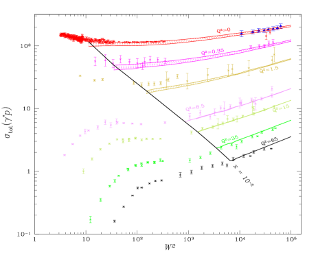
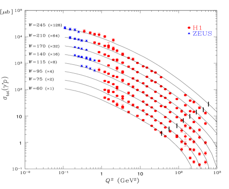
Figure 13-a	Figure 13-b

Figure 13: The description of experimental data in Gribov approach, given in Ref. [60].

A success in phenomenological description gives us hope, that the approach based on Gribov’s ideas can be used for matching of “soft” and “hard” processes for more general observables than the total cross section and, finally, will lead to selfconsistent Monte Carlo code for all values of the photon virtualities.

Golec - Bierat and Wüsthoff approach: The natural generalization of discussed attempts to describe the matching between long and short distances physics is to use the SC approach. The full description based on formulae of Eq. 12 ) - type has not been developed yet. However, Golec - Bierat and Wüsthoff [42] [43] suggested a simple phenomenological approach which incorporates the main qualitative and even quantitative feathures of the general SC calculations.

They use for the total cross section of photon - proton interaction the following formula [42]

$$\sigma(\gamma^{*}p)\,\,\,=\,\,\int\,\int d^{2}r_{\perp}\,dz\,|\Psi(Q^{2};z,r_{\perp})|^{2}\,\,\sigma(x,r_{\perp})\,\,;$$ (28)

where

$$\sigma(x,r_{\perp})\,\,\,=\,\,\,\sigma_{0}\,\,\{\,\,1\,\,\,-\,\,\,e^{-\,\frac{r^{2}_{\perp}}{R^{2}(x)}}\,\,\}\,\,.$$ (29)

$R^{2}(x)$ is a new scale for the DIS,namely, $R^{2}(x)\,\,=\,\,1/Q^{2}_{0}(x)$. Golec-Bierat and Wüsthoff use the phenomenological parameterization for $Q^{2}_{0}(x)\,\,=\,\,Q^{2}_{0}\,\,(x/x_{0})^{\lambda}$ instead of calculation that lead to Fig.6. With $\sigma_{0}\,\,=\,\,23.03\,\,mb$,$\lambda\,\,=\,\,0.288$ and $x_{0}\,\,=\,\,3.04\,10^{-4}$. Golec-Bierat and Wüsthoff successfully described both the total cross sections of the photon - proton interaction [42] as well as the cross sections of the diffractive production in DIS [43]. Fig.14 show what kind of description can be reached in such an approach, as well as the value of the typical momentum $Q_{0}(x)$ and effectivew Pomeron intercept in their model.

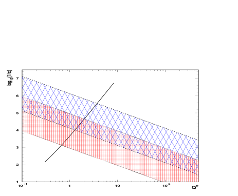
Figure 14-a	Figure 14-b

Figure 14 -c

Figure 14: Golec-Bierat and Wüsthoff approach: ( a ) the critical line $Q^{2}=Q^{2}_{0}(x)$; ( b ) the effective Pomeron intercept and (c) the description of the experimental data

This approach demonstrates that SC are a possible way of describing the matching of the “soft” and “hard” kinematic regions. On the other hand it gives a practical way to write the matching of pQCD and np QCD contribution into Monte Carlon codes.

5 Survival probability of Large Rapidity Gaps ( LRG)

Definitions and general discussion: A LRG process[61] [62] is a multiparticle production process in which no particles are produced in a large window in rapidity. The typical process of this kind is the production of two jets with high transverse momenta ($p_{1t}$ and $p_{2t}$ ) and large rapidity difference ( $y_{1}-y_{2}\,\,\gg\,\,1$ ) between them in which no hadrons are produced ( see Fig.15 ).

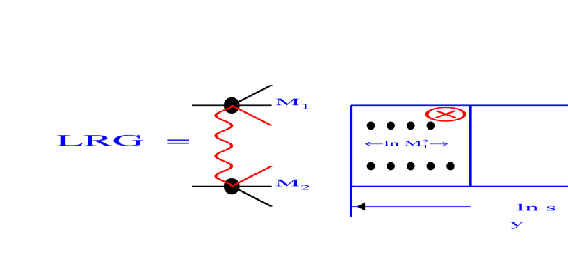
Figure 15: The lego - plot of the typical LRG process of “hard” dijets production with large rapidity gap between them where no hadrons are produced

$$p\,\,+\,\,p\,\,\,\longrightarrow\,\,$$ (30)

$$\,hadrons\,[\,Y-y_{1}\,]\,\,+\,\,jet\,[y_{1},p_{1t}\,\,+\,\,LRG\,[\,y_{1}-y_{2}\,]\,\,+\,\,jet\,[\,y_{2},p_{2t}\,]\,\,+\,\,hadron\,[\,y_{2}-0\,]\,\,.$$

Bjorken advocated that LRG processes is a unique way to measure high energy asymptotic at short distances. In our slang, we call this asymptotic the exchange of “hard” Pomeron, expressing our hope that we can calculate it in pQCD. The following observable was suggested [61] [62] to be measured experimentally ( see Fig.16 ):

$$f_{gap}\;\,\,=\;\,\,\frac{\sigma(\;\;dijet\;\;production\;\;with\;\;LRG\,\,)}{\sigma_{inclusive}(\;\;dijet\;\;production\,\,)}\,\,.$$ (31)

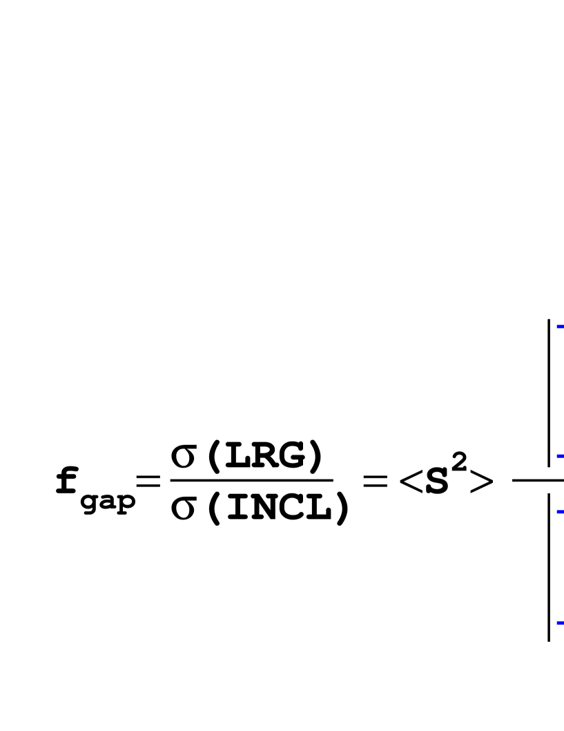
Figure 16: General expression for $f_{gap}$.

Unfortunately, the experimental obsevable $f_{gap}$ does not measure the contribution of the “hard” Pomeron but has a factor[62] $<|S^{2}|>$ which we call the survival probability of LRG and which is the subject of this section. We will try to answer the following questions:

1. What is the survival probability of LRG processes  ?

2. What is the value of survival probability  ?

3. How well can we estimate this value   ?

4. What is the energy dependence of survival probability  ?

Data: We start to discuss the problem of the survival probability citing all experimental data on this subject given by D0[63] amd CDF[64].

	D0[63]	CDF[64]
$f_{gap}(\,\sqrt{s}\,\,=\,\,1800\,GeV\,)$	0.54  $\pm$  0.17 $\%$	1.13  $\pm$  0.16 $\%$
$f_{gap}(\,\sqrt{s}\,\,=\,\,640\,GeV\,)$	1.85  $\pm$  0.38 $\%$	2.7  $\pm$  0.9 $\%$
$R_{gap}\,\,=\,\,\frac{f_{gap}(\,\sqrt{s}\,\,=\,\,630\,GeV\,)}{f_{gap}(\,\sqrt{s}\,\,=\,\,1800\,Gev\,)}$	3.4  $\pm$  1.2	2.4 $\pm$ 0.9
$R_{S}\,\,=\,\,\frac{\langle\mid S\mid^{2}\rangle(\,\sqrt{s}\,\,=\,\,630\,GeV\,)}{\langle\mid S\mid^{2}\rangle(\,\sqrt{s}\,\,=\,\,1800\,GeV\,)}$	2.2 $\pm$ 0.8	???

We can learn two important properties of $\langle\mid S\mid^{2}\rangle$:

1. The value of $\langle\mid S\mid^{2}\rangle$ is small ( $\langle\mid S\mid^{2}\rangle\,\,\mathrel{\hbox to0.0pt{\lower 4.0pt\hbox{\hskip 1.0pt$\sim$}\hss}\raise 1.0pt\hbox{$<$}}\,\,10\,\%$ ) because all estimates [66] show that the ratio of “hard” Pomeron to inclusive dijet production is about 10 - 20% ;

2. $\langle\mid S\mid^{2}\rangle$ decreases rapidly with energy. At least we have to blame the survival probability for experimentally observed fast decreasing of $f_{gap}$, since the ratio of “hard” Pomeron to inclusive dijet production can only increase in pQCD.

It should be stressed that only the first data on $f_{gap}$ in DIS [65] have appeared, this does not allow us to make any conclusions on the energy behaviour of $\langle\mid S\mid^{2}\rangle$ but tell us that the value of the survival probability, is much higher ( $\langle\mid S\mid^{2}\rangle\,\,\approx\,\,50-70\%$ ) than in hadron - hadron collisions.

Two source of survival probability: It turns out that the survival probability $\langle\mid S\mid^{2}\rangle$ can be written as a product of two factor. Each of them has a different physical meaning.

$$\langle\mid S\mid^{2}\rangle\,\,\,=\,\,\,\langle\mid S_{bremsstrahlung}(\Delta y=|y_{1}-y_{2}|)\mid^{2}\rangle\,\,\times\,\,\langle\mid S_{spectators}(s)\mid^{2}\rangle$$ (32)

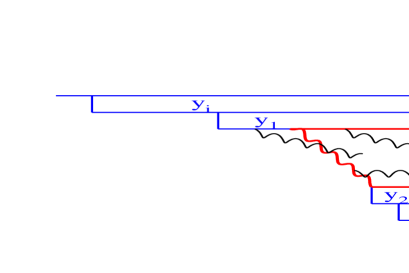
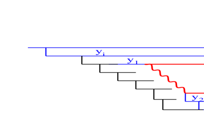
Figure 17-a	Figure 17-b

Figure 17: Examples of processes that lead to $\langle\mid S_{bremsstrahlung}\mid^{2}\rangle$. ( Fig.17-a ) and to $\langle\mid S_{spectator}|\mid^{2}\rangle$ ( Fig. 17-b ).

The first factor in Eq.( 32 ) ( $\langle\mid S_{bremsstrahlung}\mid^{2}\rangle$ ) describes the probability that the LRG will not be filled by emission of bremsstrahlung gluons from partons, taking part in the “hard” interaction (see Fig. 17-a ). It depends mostly on the value of the rapidity gap [68]. The second factor( $\langle\mid S_{spectator}\mid^{2}\rangle$ ) appears to take into account the probability that no parton with $x_{i}\,\,>\,\,x_{1}$ will have an inelastic interaction with any parton with $x\,\,<\,\,x_{2}$ (see Fig. 17-b ). From Fig. 17-b one can see that this factor depends on the total energy of the process ( $s$ ) [62] [69][70][72]. Different physics behind these two factors lead to a different theoretical status for their calculations. For calculations of the value of $\langle\mid S_{bremsstrahlung}\mid^{2}\rangle$ the pQCD thechnique could be and has been developed [68]. Only a part of $\langle\mid S_{spectator}\mid^{2}\rangle$ can be controled by pQCD, while the estimates for most of this factor could only be made in npQCD. In pratice, it means that we must rely on high energy phenomenology in our attempts to provide an estimate for $\langle\mid S_{spectator}\mid^{2}\rangle$.

Before discussing what we have learned about $\langle\mid S_{spectator}\mid^{2}\rangle$ we would like to remind the reader that all corrections for interactions of two groups of parton ( see Fig. 17-b ) cancel due to Abramovski-Gribov-Kancheli cutting rules [67].

Survival Probability in the Eikonal Model: In order to understand the main features of the survival probability, let us consider it in the simplest phenomenological model for the “soft” interaction - the Eikonal model.

$\bullet$    Main assumptions:

• Only the fastest parton interacts with “wee” partons

• Hadrons are correct degrees of freedom at high energy

• $\frac{\sigma_{SD}+\sigma_{DD}}{\sigma_{el}}\,\,\ll\,\,1$
  

• Oversimplified final state

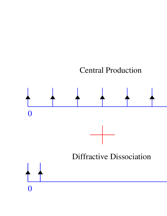
Figure 18: The rapidity structure of the typical event in the Eikonal model.

• Simple form of unitarity :

  $$2\,Ima_{el}(s,b)\,\,=\,\,\mid a_{el}(s,b)\mid^{2}\,\,+\,\,G_{in}(s,b)\,\,.$$ (33)

• Solution:

  $$a_{el}\,\,=\,\,i\,[\,1\,-\,e^{-\frac{\Omega(s,b)}{2}}\,]\,;$$ (34)

  $$G_{in}(s,b)\,\,=\,\,1-e^{-\Omega(s,b)}\,;$$ (35)

  where $\Omega(s,b)$ is an orbitrary real function.

• Simple parameterization  :

  $$\Omega(s,b)\,\,\,=\,\,\frac{\sigma_{0}}{\pi R^{2}(s)}\,\,(\,\frac{s}{s_{0}}\,)^{\Delta_{P}}\,\,e^{-\frac{b^{2}}{R^{2}(s)}}\,\,=\,\,\nu(s)\,\,e^{-\frac{b^{2}}{R^{2}(s)}}$$ (36)

• Analytical formulae for “soft” observable :

  $$\sigma_{tot}=2\int d^{2}b(1-e^{-\Omega(s,b)/2})=2\pi R^{2}(s)\,[\,ln(\frac{\nu(s)}{2})+C-Ei(-\frac{\nu(s)}{2})\,]\,;$$ (37)

  $$\sigma_{in}=\int d^{2}b(1-e^{-\Omega(s,b)})=\pi R^{2}(s)\,[\,ln(\nu(s))+C-Ei(-\nu(s))\,]\,;$$ (38)

  $$\sigma_{el}=\sigma_{tot}-\sigma_{in}=\pi R^{2}(s)\,[\,ln(\frac{\nu(s)}{4})+C+Ei(-\nu(s))-2Ei(-\frac{\nu(s)}{2})\,]\,.$$ (39)

• A simple formula for survival probability :

  $$<\mid S_{spectator}\mid^{2}>=\frac{\int d^{2}b\Gamma_{H}(b)P(s,b)}{\int d^{2}b\Gamma_{H}(b)}\,\,,$$ (40)

  with $\Gamma_{H}(b)=\frac{1}{\pi R^{2}_{H}}e^{-\frac{b^{2}}{R^{2}_{H}}}$

• Analitycal form of $<\mid S_{spectator}\mid^{2}>$ :

  $$<\mid S_{spectator}\mid^{2}>=\frac{a(s)\gamma[a(s),\nu(s)]}{[\nu(s)]^{a(s)}}$$ (41)

  with $a(s)=\frac{R^{2}_{S}(s)}{R^{2}_{H}}$.

Survival Probability in the Eikonal Model ( comparison with experiment ):

To get more reliable estimates for the value and energy dependance of $<\mid S_{spectator}\mid^{2}>$ we tried to extract all parameters directly from the experimental data [70]. The first observation ( see Eqs.( 37 ) - ( 39 ) ) is that the ratio

$$R_{el}(\nu)\,\,=\,\,\frac{\sigma_{el}}{\sigma_{tot}}$$ (42)

is a function of the only parameter $\nu$. Therefore, we can use the experimental data on $R_{el}$ to fix $\nu$ at particular value of energy ( see Fig.19 ).

To fix the value of $a(s)$ we used the data on J/$\Psi$ production[71] which shows two differents slopes in $t$-dependence for elastic and inelastic processes ( see Fig. 20-a ). These data can be used to extract the value of $R^{2}_{H}=8\,GeV^{-2}$ ( see Ref. [70] ).

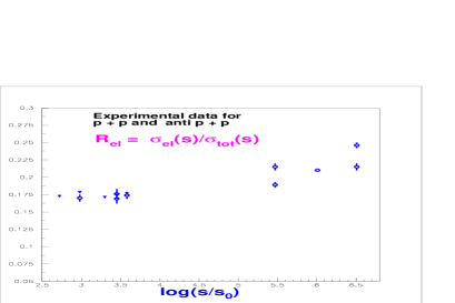
Figure 19-a	Figure 19-b

Figure 19: Experimental data ( Fig.19-a ) and the Eikonal model predictions ( Fig.19-b ) for $R_{el}=\frac{\sigma_{el}}{\sigma_{tot}}$ .

Using “soft” phenomenology for $R^{2}(s)$ [70] we obtained prediction for the survival probability given in Fig.20. One can see that the Eikonal model reproduces both the experimental value and the energy dependence of the survival probability.

Figure 20-a	Figure 20-b

Figure 20: J/$Psi$ production (Fig.20-a ) and the survival probability $<\mid S_{spectator}\mid^{2}>$ in the Eikonal model ( Fig.20-b )

More general approach to calculation of $\mathbf{\langle\mid S_{spectator}\mid^{2}\rangle}$.

In Ref. [72] a more general approach has been developed to calculation of $<\mid S_{spectator}\mid^{2}>$ which based on the following assumptions:

• Only the fastest parton interacts with the target   ;

• Hadrons are not correct degrees of freedom  ;

• $\frac{\sigma_{DD}(\,M\,>\,M_{0}\,)}{\sigma_{el}}\,\,\ll\,\,1$  ;

• Oversimplified final state: central production ( uniform in rapidity) and elastic + diffractive production with small masses.

One can see that all the above assumptions are very close to the Eikonal model, and the difference actually is only in the way of how the diffractive production processes are treated. In the model of Ref. [72] we assume that the correct degrees of freedom at high energy are not hadrons but some different states which are described by wave functions $\Psi_{1}$ and $\Psi_{2}$. Our interaction matrix is diagonal

$$<\Psi_{n}\times\Psi_{m}|{\mathbf{T}}|\Psi_{n^{\prime}}\times\Psi_{m^{\prime}}>\,\,\,=\,\,\,A_{n,m}(s,b_{t})\,\delta(n-n^{\prime})\,\delta(m-m^{\prime})\,\,,$$ (43)

and only for $A_{n,m}$ ( not for hadrons ) unitarity has a form:

$$2\,\,Im\,\,A_{n,m}(s,b_{t})\,\,\,=\,\,\,|A^{2}_{n,m}(s,b_{t})|^{2}\,\,\,+\,\,G^{in}_{n,m}(s,b_{t})\,\,.$$ (44)

Produced hadrom and a diffractive state have the following wave functions:

$$\Psi_{hadron}\,\,\,=\,\,\,\alpha\,\,\Psi_{1}\,\,\,+\,\,\,\beta\,\,\Psi_{2}\,\,;$$ (45)

$$\Psi_{D}\,\,\,=\,\,\,-\,\beta\,\,\Psi_{1}\,\,\,+\,\,\,\alpha\,\,\Psi_{2}\,\,.$$ (46)

Therefore, three channels were taken into account in this model, namely, elastic scattering, single and double diffractice production while only elastic rescatterings were included in the Eikonal model.

Using the Eikonal - like parameterization ( see Fig.21 ), the three channel model leads to the prediction for the value and energy dependence of $\langle\mid S_{spectator}\mid^{2}\rangle$ given in Fig.22. One can see that this model can reproduce the experimental data including the energy dependence.

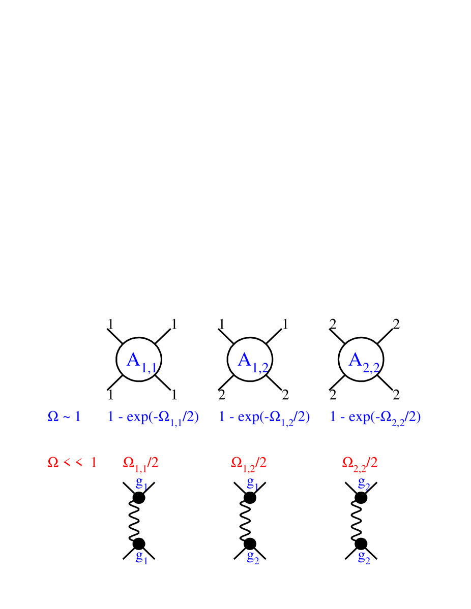
Figure 21: The Eikonal - like parameterization in the three channel model.

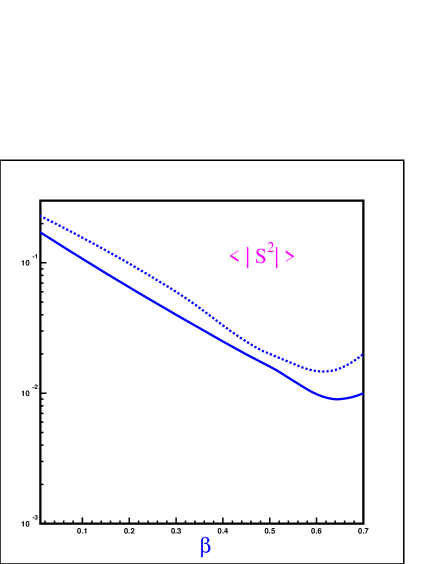
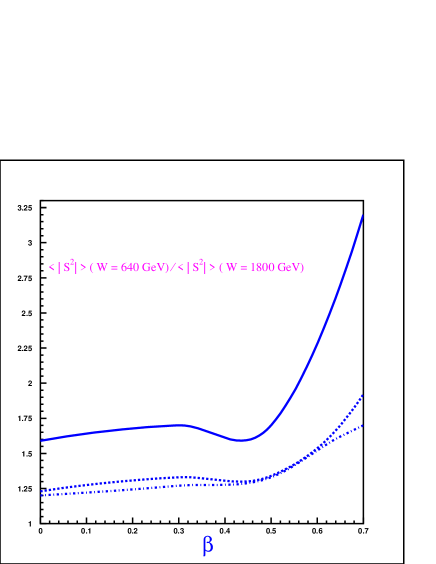
Figure 22-a	Figure 22-b

Figure 22: The value ( Fig.22-a ) of survival probability $<\mid S_{spectator}\mid^{2}>$ at $\sqrt{s}=W=1800\,GeV$ and the ratio $<\mid S(\,W\,=\,640\,GeV\,)\mid^{2}>/<\mid S(\,W\,=\,1800\,GeV\,)\mid^{2}$ ( Fig.22-b ) versus $\beta$ in the three channel model.

Summarizing the experience dealing with three channel model, we can conclude that:

• Accuracy of the three channel model, in principle, is much better than in the Eikonal Model, but still we do not know what to do with diffraction in the region of large mass ( $M\,\,\approx\,\,s$ )  ;

• The scale of SC is not given by $R_{D}\,\,\,=\,\,\,\frac{\sigma_{el}\,\,+\,\,\sigma_{SD}\,\,\,+\,\,\,\sigma_{DD}}{\sigma_{tot}}\,\,,$ but rather by the separate ratios

  $R_{el}\,\,=\,\,\frac{\sigma_{el}}{\sigma_{tot}}$

  $R_{SD}\,\,=\,\,\frac{\sigma_{SD}}{\sigma_{tot}}$

  $R_{DD}\,\,=\,\,\frac{\sigma_{DD}}{\sigma_{tot}}$

• The small value of the survival probability as well as its strong energy dependence appear naturally in this approach  ;

• The parameters that have been used are in agreement with the more detailed fit of the experimental data  ;

• Questions to experimentalists:

  1. What is $R_{el}$ at $\sqrt{s}$ equal to 630 GeV ? 1800 GeV ? Tevatron runII energy ?

  2. What is the value for $R_{SD}$ at $\sqrt{s}$ equal to 630 GeV ? 1800 GeV ? Tevatron runII energy ?

  3. What is the value for $R_{DD}$ at $\sqrt{s}$ equal to 630 GeV ? 1800GeV ? Tevatron runII energy ?

     

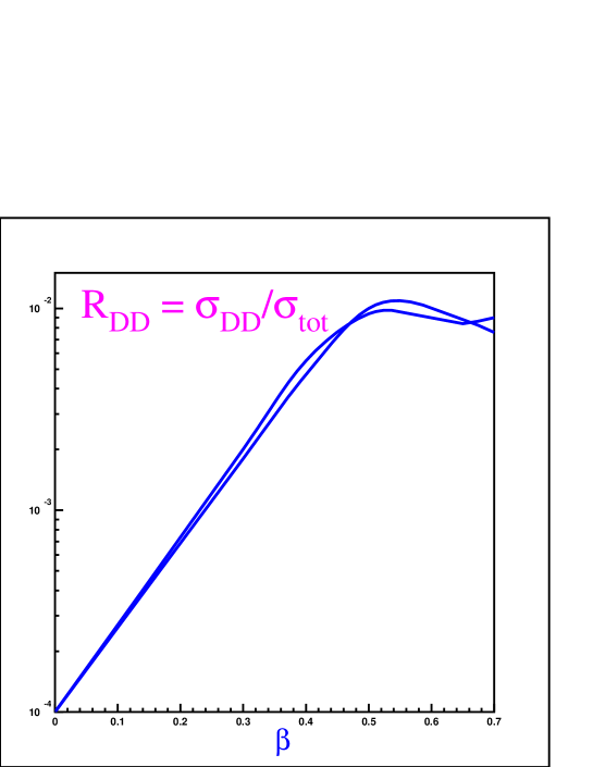
     Figure 23: The three channel model predictions for double diffractive dissociation ( $R_{DD}=\sigma_{DD}/\sigma_{tot}$.

  4. What is the value of the single diffraction cross section in the region of large masses at $\sqrt{s}$ equal to 630 GeV ? 1800 GeV ? Tevatron runII energy ?

Q  &  A :

Q:	Have we developed a theory for $\langle\mid S_{spectator}\mid^{2}\rangle$ ?
A:	No, there are only models on the market .
Q:	Can we give a reliable estimates for the value of $\langle\mid S_{spectator}\mid^{2}\rangle$  ?
A:	No, we have only rough estimates based on the Eikonal - type models.

Q:	Can we give a reliable estimates for the energy behaviour of $\langle\mid S_{spectator}\mid^{2}\rangle$  ?
A:	No, but we understand that $\langle\mid S_{spectator}\mid^{2}\rangle$ could decreases steeply with energy.
Q:	Why are you talking about $\langle\mid S_{spectator}\mid^{2}\rangle$ if you can do nothing ?
A:	Because:

• Dealing with models we have learned what questions we should ask experimentalists to improve our calculations;

• We learned what problems we need to solve theoretically to provide reliable estimates;

• We understood what kind of questions could be answered in LRG experiments;

• We are on the way to an understanding in what experiments our accuracy is enough, to get interesting information on the high energy scattering amplitude at short distances.

Survival Probability in DIS: I hope, that I have explained to you that we do not have a consistent theoretical approach to the calculation of $\langle\mid S_{spectator}\mid^{2}\rangle$ for hadron - hadron collisions. The natural question to ask is : can the theoretical situation be better for DIS where the “short” distances can give the major contribution?

To answer this question let us consider first two examples of the LRG processes in DIS: the diffractive dissociation ( DD ) and one-side dijets production in DD ( see Fig.24 ).

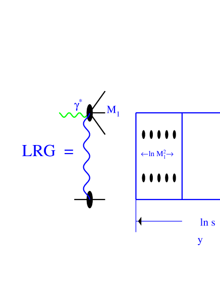
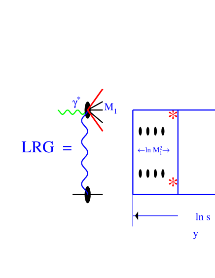
Figure 24-a	Figure 24-b

Figure 24: Lego - plots for DD ( Fig.24-a) and one-side dijets production in DD ( Fig.24-b ) in DIS.

Fig.25 shows the parton interaction which can occur for one-side dijets production in DD.

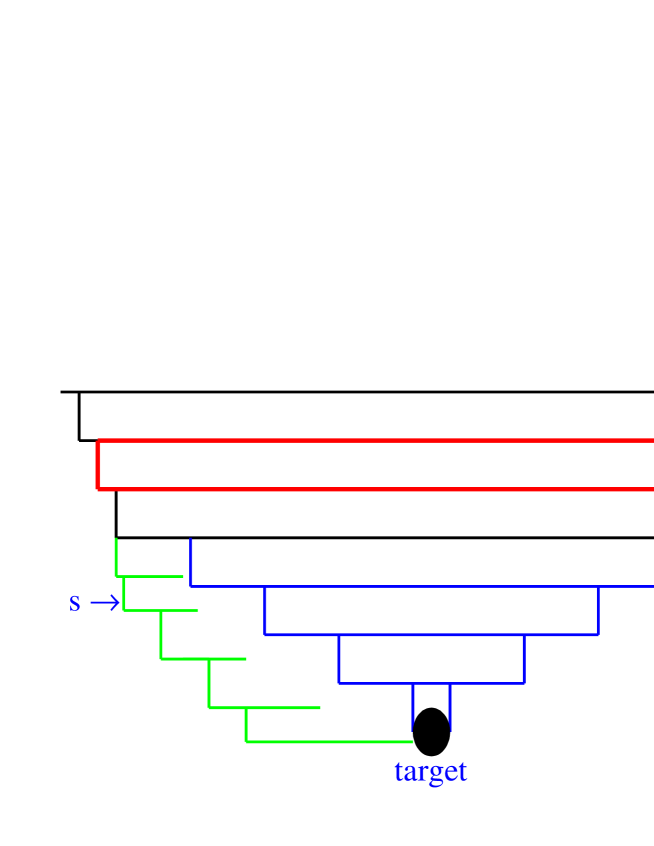
Figure 25: Picture of parton interactions for one-side dijets production in DD in DIS.

Using the main properties of the parton cascade ( mostly the AGK - cutting rules [67] ) we can make three observation on the survival probability for this process:

1. Survival probability for one - side dijets depend on $Q^{2}$ and $x_{B}$, but does not depend on $p_{t}$ and $x_{1}$  ;

2. Survival probability is not big in comparison with LRG survival probability in proton - proton collisions  ;

3. For large $Q^{2}$ the survival probability can be calculated in pQCD  .

In the Glauber - Mueller approach the cross section of virtual photon - proton interaction can be written in the form [73] [74]:

$$\sigma(\gamma^{*}p)\,=\,\int\int\,d^{2}r_{t}\,dz\,\,|\Psi(Q^{2};z,r_{t})|^{2}\,\sigma(x,r^{2}_{t})\,\,;$$ (47)

with

$$\sigma(x,r^{2}_{t})\,\,=\,\,2\,\,\int\,\,d^{2}b_{t}\,\,[\,\,1\,\,\,-\,\,\,e^{-\,\,\frac{\Omega(r^{2}_{t},x_{B};b_{t})}{2}}\,\,]\,\,;$$ (48)

where $\Psi$ is the wave function of the virtual photon and

$$\Omega(r^{2}_{t},x_{B};b_{t})\,\,\,=\,\,\,\frac{16\pi\alpha_{S}}{3}\,r^{2}_{t}\,\,x_{B}\,G(x_{B},\frac{r^{2}_{t}}{4})\,\,\frac{1}{R^{2}}\,e^{-\,\frac{b^{2}_{t}}{R^{2}}}\,\,.$$ (49)

$R^{2}\,=\,2\,B^{DD}(x_{B})$ where

$$\frac{\frac{d\sigma_{DD}}{dt}(t)}{\frac{d\sigma_{DD}}{dt}(t=0)}\,\,=\,\,e^{-B^{DD}\,|t|}$$

and this parameter is closely related to non pertutbative physics. At the moment we can use the experimental data on the slope of the DD processes in DIS. It should be stressed that factoring out the $b_{t}$ - dependence can be justified in QCD using the factorization theorem [75].

The formula for the survival probability is a direct generalization of Eq.( 40 ) in the Eikonal model, namely:

$$\langle\mid S_{spectator}\mid^{2}\rangle\,\,\,=\,\,\,\frac{\int\int\int d^{2}r_{t}\,dz\,d^{2}b_{t}\,\,|\Psi(Q^{2};z,r_{t})|^{2}\,e^{-\,\,\Omega(r^{2}_{t},x_{B};b_{t})}\,\,e^{-\,\,\frac{2\,b^{2}_{t}}{R^{2}}}}{\int\int\int d^{2}r_{t}\,dz\,d^{2}b_{t}\,\,|\Psi(Q^{2};z,r_{t})|^{2}\,\,\,e^{-\,\,\frac{2\,b^{2}_{t}}{R^{2}}}}$$ (50)

The calculations [40], using Eqs. ( 47 ) - ( 50, shows that the survival probability is much less in DIS than in hadron - hadron collisions ( see Fig.26, where $D^{2}_{T}\equiv S^{2}$ is plotted for the transverse polarized induced photon reactions with LRG ).

Figure 26-a	Figure 26-b

Figure 26: The survival probability $\langle\mid S_{spectators}\mid^{2}\rangle\,\equiv\,D^{2}_{T}$ in DIS versus $x$ ( Fig.26-a ) and $Q^{2}$ ( Fig.26-b ).

Multiparticle production in DIS: Shadowing corrections or, in other words, the rescatterings of quark - antiquark pair in a target lead to a new predictions for the processes of multiparticle productions. Namely, it gives probabilities for production of several parton showers. For every parton shower we can use the Monte Carlo code based on the evolution equations, while the probability for configuration with $n$ - parton showers can be calculated, using the following simple formula:

$$\sigma_{n}\,\,\,=\,\,\int\,\,d^{2}r_{t}dzd^{2}b_{t}|\Psi(Q^{2},r_{t},z)|^{2}\,\,\frac{\Omega^{n}}{n!}\,e^{-\Omega}$$ (51)

Fig.26 shows the first three terms in our decomposition of the multiparticle production in the parton showers: diffraction dissociation, one parton shower and two parton showers productions. For better understanding, in Fig.26 the probability of each configuration in the limit of small $\Omega$ is also given.

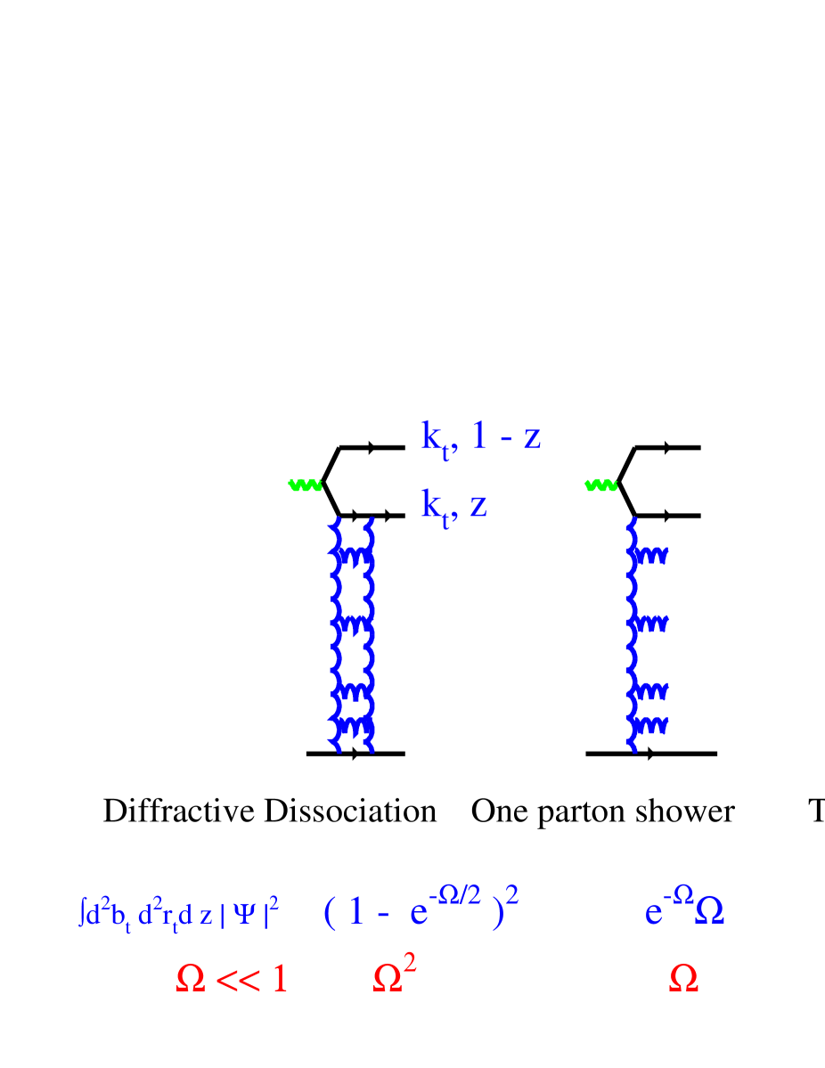
Figure 27: The first three terms in parton showers decomposition.

I am firmly believe that such a decomposition will be very useful for writing Monte Carlo programs.

6 Conclusions

In this talk I tried to give you a picture of recent progress in low $x$ physics. I chose the subject which, I hope, would be useful for Monte Carlo experts. Let me summarize in short the present situation in four subjects that I have discussed here:

1. We are on the right track in understanding of the next-to-leading BFKL Pomeron, but, at the moment, we cannot guarantee any calculations of the parameters of the BFKL Pomeron;

2. First experimental indications of the strong shadowing corrections have appeared in energy behaviour of the diffraction dissociation cross sections in DIS and in the $Q^{2}$ - behaviour of the $F_{2}$ - slope ( Caldwell plot ). We hope, that these data will stimulate the new experimental systematic search of SC, as well as the creation of the new Monte Carlo codes, that will include the SC and physics, induced by them;

3. Considerable progress, based on Gribov’s ideas, has been achieved in describing the matching between the non-perturbative “soft” processes, and the perturbative “hard” ones in photon - proton interactions. We firmly believe that this progress will be useful both for future non-perturbative approaches in QCD and for creating new Monte Carlo program, which take this matching into account;

4. We can estimate the survival probability in hadron - hadron collisions only in rather primitive models, which can reproduce the basic experimental data on it. The prediction for the survival probability in DIS are more solid from theoretical point of view, but the experimental information is so poor that we cannot compare the main features of our calculations with the data. We think that time has come to include in Monte Carlo codes the decomposition of multiparticle production process in the series of multi parton showers production, which is closely related the the value of the survival probability.

Acknowlegments: I am very grateful to E. Gotsman and U. Maor for permanent useful discussions on the subject which only partly were reproduced in our common papers. I would like to thank E.Naftali for preparing Fig.9 specially for this talk. I would like also to thank all participants of the MC Workshop whose discussions which were useful and supportive for me.

References

-
[1]
E.A. Kuraev, L.N. Lipatov and V.S. Fadin, Sov. Phys. JETP 45,
199 (1977);
Ya.Ya. Balitskii and L.V. Lipatov, Sov. J. Nucl. Phys. 28, 822 (1978);
L.N. Lipatov, Sov. Phys. JETP 63, 904 (1986). -
[2]
V.N. Gribov and L.N. Lipatov,Sov. J. Nucl. Phys. 15, 438
(1972);
L.N. Lipatov, Yad. Fiz. 20, 181 (1974);
G. Altarelli and G. Parisi, Nucl. Phys. B 126, 298 (1977);
Yu.L. Dokshitser, Sov. Phys. JETP 46, 641 (1977). - [3] E. Levin, TAUP-2501-98, hep-ph/9806228, Nucl. Phys.B ( in press ).
- [4] D.Yu. Ivanov et al., Phys. Rev.D 58, 2821 (1998).
- [5] E. Laenen and E. Levin, Ann. Rev. Nucl. Phys. 44, 199 (1994).
- [6] A.M. Cooper-Sarkar, R.C.E. Devenish and A. De Roeck, Int.J.Mod.Phys. A 13, 3385 (1998).
- [7] H.Abramowicz and A. Caldwell, hep-ex/9903037, Rev. Mod. Phys. ( in press ).
-
[8]
H1 Collaboration,S. Aid et. al.,Phys. Lett. B 356, 118 (1995);
ZEUS Collaboration, J. Breitweg et al., DESY-98-050. - [9] J. Bartels et al., Phys. Lett. B 384, 300 (1996).
-
[10]
M. Ciafaloni, Nucl. Phys. B296,249 (1987);
S. Catani, F. Fiorani and G. Marchesini, Phys. Lett. B 234,339 (1990),Nucl. Phys. B336,18 (1990). - [11] V.S. Fadin and L.N. Lipatov, Phys. Lett. B 429, 127 (1998).
-
[12]
M. Ciafaloni, Phys. Lett. B 429, 363 (1998)
G. Camici and M. Ciafaloni, Phys. Lett. B 430, 349 (1998). - [13] J. Blumlein and A. Vogt, Phys. Rev.D 57, 1 (1998);D 58, 014020 (1998).
- [14] D.A. Ross, Phys. Lett. B 431, 161 (1998).
- [15] E. Levin, Nucl. Phys.B 453, 303 (1995).
- [16] Yu. V. Kovchegov and A.H. Mueller, Phys. Lett. B 439, 428 (1998).
- [17] N. Armesto, J. Bartels and M.A. Braun, Phys. Lett. B 442, 459 (1998).
- [18] G.P.Salam, J.High Energy Phys. 9807, 019 (1998).
-
[19]
M. Ciafaloni, invited talk at IX Int. Workshop on Small x Physics
and Light - front Dynamics in QCD,
July 6 - 15,1998,
St.Petersburg, Russia;
G. Camici and M. Ciafaloni, Phys. Lett. B 412, 396 (1997); Phys. Lett. B 395, 118 (1997); Nucl. Phys.B 496, 305 (199);
M. Ciafaloni and D. Colferai,hep-ph/9812366. - [20] B. Andersson, G. Gustafson and J. Famuelsson, Nucl. Phys.B 467, 443 (1996).
- [21] J.R. Forshaw, D.A. Ross and A. Sabio Vera, CERN-TH/99-64,9903390.
- [22] C.R. Schmidt, MSUHEP-90122, Jan. 24, 1999, hep-ph/9901397.
- [23] J.R. Forshaw, G.P. Salam and R.S. Thorne, MC-TH-98/23, hep-ph/9812304.
- [24] H. Kharraziha and L. Lönnblad, JHEP 3, 6 (1998), hep-ph/9709424,
- [25] ZEUS collaboration, Breitweg J. et al., DESY 98 - 121, Eur. Phys. J (in press ).
- [26] L. V. Gribov, E. M. Levin and M. G. Ryskin, Phys.Rep. 100, 1 (1983).
- [27] A.H. Mueller and J. Qiu, Nucl. Phys. B 268, 427 (1986).
- [28] A.H.Mueller: Nucl. Phys. B 335, 115 (1990).
- [29] Yu. V. Kovchegov, NUC-MN-99/1 - T, hep-ph/9901281.
- [30] A.L. Ayala, M.B. Gay Ducati and E.M. Levin, Nucl. Phys. B 493, 305 (1997).
- [31] A.L. Ayala, M.B. Gay Ducati and E.M. Levin, Nucl. Phys. B 510, 355 (1998).
- [32] L. McLerran and R. Venugopalan: Phys. Rev. D 49, 2233, 3352 (1994); D 50, 2225 (1994); D 53, 458 (1996).
-
[33]
J. Jalilian-Marian, A. Kovner, A. Leonidov and H. Weigert,
Phys. Rev.D 59, 014014, 034007 (1999); Nucl. Phys.B 504, 415 (1997);
J.Jalilian-Marian, A. Kovner, L. McLerran and H. Weigert, Phys. Rev. D 55, 5414 (1997);
A. Kovner, L. McLerran and H. Weigert, Phys. Rev.D 52, 3809, 6231 (1995). -
[34]
Yu. Kovchegov, Phys. Rev. D 54, 5463 (1996); D 55, 5445
(1997);
Yu. V. Kovchegov and A.H. Mueller, Nucl. Phys.B 529, 451 (1998);
Yu. V. Kovchegov, A.H. Mueller and S. Wallon, Nucl. Phys.B 507, 367 (1997). -
[35]
H1 Collaboration, T. Ahmed et al., Phys. Lett. B 348, 681
(1995);
H1 Collaboration, C. Adloff et al., Z. Phys.C 76, 613 (1997). -
[36]
ZEUS collaboration, M. Derrick et al., Z. Phys.C 68, 569 (1995);
ZEUS collaboration, J. Breitweg et al, Eur. Phys. J. C 6, 43 (1999). - [37] A. Donnachie and P.V. Landshoff, Nucl. Phys. B 244, 322 (1984); B 267, 690(1986); Phys. Lett. B 296, 227 (1992); Z. Phys. C 61, 139 (1994).
- [38] J. Bartels, H. Lotter and M. Wüsthoff, Phys. Lett. B 379, 239 (1996).
- [39] N. Nikolaev and B.G. Zakharov, Z. Phys.C 53, 331 (1992).
- [40] E. Gotsman, E. Levin and U. Maor, Nucl. Phys.B 493, 354 (1997).
- [41] E. Gotsman, E. Levin, U. Maor and E. Naftali, Nucl. Phys.B 539, 535 (1999).
- [42] K. Golec-Biernat and M. Wüsthoff, Phys. Rev.D 59, 014017 (1999).
- [43] K. Golec-Biernat and M. Wüsthoff, DTP-99-20,hep-ph/9903358.
- [44] Yu. V. Kovchegov and L. McLerran, NUC-MN-99/2-T, hep-ph/9903246.
- [45] M. Abramovitz and I.A. Stegun, Handbook of Mathematical Functions.
- [46] A.L. Ayala, M.B. Gay Ducati and E.M. Levin, Phys. Lett. B 388, 188 (1996).
- [47] ZEUS collaboration, J. Breitweg et al., DESY 98 - 121, Eur. Phys. J. ( in press ).
- [48] A.H. Mueller, plenary talk at DIS’98 eds. Ch. Coremans and R. Roosen, WS, 1998; CU-TP-937-99, hep-ph/9904404.
- [49] E. Gotsman, E. Levin and U. Maor, Phys. Lett. B 425, 369 (1998).
-
[50]
H. Abramowicz, E. Levin, A. Levy and U. Maor, Phys. Lett. B 269, 465 (1991);
H. Abramowicz and A. Levy, DESY 97-251, hep-ph/9712415. - [51] A.D. Martin, R.G. Roberts, W.J. Stirling and R.S. Thorne, Eur.Phys.J. C 4, 463 (1998).
-
[52]
H1 Collaboration: C. Adloff et al.,Nucl. Phys.B 497, 3 (97);
H1 Collaboration: S. Aid et al.,Nucl. Phys.B 470, 3 (96). - [53] ZEUS Collaboration: J. Breitweg et al., Phys. Lett. B 407, 432 (1997).
- [54] V.N. Gribov, Sov. Phys. JETP 30, 709 (1970).
-
[55]
J.J. Sakurai and D. Schildknecht, Phys. Lett. B 40, 121 (1972);
B. Gorczyca and D. Schildknecht, Phys. Lett. B 47, 71 (1973)’ -
[56]
E.M. Levin and L.L. Frankfurt, JETP Letters 3, 652 (1965);
H.J. Lipkin and F. Scheck, Phys. Rev. Lett. 16, 71 (1966);
J.J.J. Kokkedee, The Quark Model , NY, W.A. Benjamin, 1969. - [57] E. Gotsman, E. Levin and U. Maor, Eur. Phys. J. C 5, 303 (1998).
- [58] A.D. Martin, M.G. Ryskin and A.M. Stasto, Eur.Phys.J. C 7,643 (1999).
- [59] B. Badelek and J. Kwiecinski, ZPC 43, 251 (1989);Phys. Lett. B 295, 263 (1992);Phys. Rev.D 50, R4 (1994).
- [60] E. Gotsman, E. Levin, U. Maor and E. Naftali, TAUP 2573/99, hep-ph/9904277.
-
[61]
Yu. L. Dokshitzer, V. Khoze and S.I. Troyan, Proc.“Physics in
Collisions 6”, p. 417, ed. M. Derrick, WS 1987;
Sov. J. Nucl.
Phys. 46, 712 (1987);
Yu. L. Dokshitzer, V. Khoze and T. Sjostrand, Phys. Lett. B 274, 116 (1992). - [62] J. D. Bjorken, Int. J. Mod. Phys. A 7, 4189 (1992); Phys. Rev. D 47, 101 (1993).
-
[63]
D0 Collaboration, S. Abachi et al., Phys. Rev. Lett. 72,
2332 (1994); Phys. Rev. Lett. 76, 734 (1996) 734;
PLB 440, 189 (1998);
A. Brandt, “Proceedings of the 4th Workshop on Small-x and Diffractive Physics”,Sept. 17-20, 1998, FNAL,p.461. - [64] CDF Collaboration; F. Abe et al., Phys. Rev. Lett. 74, 855 (1995); 80, 1156 (1998); 81, 5278 (1998).
-
[65]
H1 collaboration, C. Adloff rt al., DESY 98-092, Eur. Phys. J. (
in press );
ZEUS collaboration, J. Breitweg et al., Eur. Phys. J. C 5 , 41 (1998). -
[66]
V. Del Duca and W. K. Tang, Phys. Lett. B312, 225 (1995);
W. Buchmüller and A. Hebecker, Phys. Lett. B355, 573 (1995);
O. J. P. Eboli, E. M. Gregores and F. Halzen, preprint MADPH-97-995 (1997),hep-ph/9708283;
R. Oeckl and D. Zeppenfeld, preprint MADPH-98-1024 (1998), hep-ph/9801257. - [67] V.A. Abramovski, V.N. Gribov and O.V. Kancheli, Sov. J. Nucl. Phys. 18, 308 (1973).
-
[68]
A.D. Martin, M.G. Ryskin and V.A. Khoze, Phys.Rev. D 56,
5867 (1997), Phys. Lett. B 401, 330 (1997);
G. Oderda and G. Sterman, Phys.Rev. Lett. 81, 3591 (1998). -
[69]
E. Gotsman, E. Levin and U. Maor, Phys.Rev. D 48,
209 (1993);
E. Levin, Phys.Rev. D 48, 2097 (1993);
R.S. Fletcher, Phys.Rev. D 48, 5162 (1993);
A. Rostovtsev and M.G. Ryskin, Phys. Lett. B 390, 375 (1997). - [70] E. Gotsman, E. Levin and U. Maor, Phys. Lett. B 438, 229 (1998).
-
[71]
S. Aid et al.,H1 Collaboration, Nucl. Phys. B 472, 3 ( 1996
);
M. Derrick et al., ZEUS Collaboration, Phys. Lett. B 350, 120 ( 1996 ). - [72] E. Gotsman, E. Levin and U. Maor, TAUP 2561-99, hep-ph/9902294.
- [73] E.M. Levin and M.G.Ryskin, Sov.J. Nucl. Phys. 45, 150 (1987).
- [74] A.H. Mueller, Nucl. Phys.B 335, 115 (1990).
- [75] J.C. Collins, D.E. Soper and G. Sterman, Nucl. Phys. B 308, 833 (1988).