Analyzing powers in inclusive pion production in high energy transversely polarized proton-proton collisions are studied theoretically in the framework of the quark recombination model. Calculations by assuming the SU(6) spin-flavor symmetry for the nucleon structure disagree with the experiments. We solve this difficulty by taking into account the realistic spin distribution functions of the nucleon, which differs from the SU(6) expectation at large $x$, with a perturbative QCD constraint on the ratio of the unpolarized valence distributions, $u/d\rightarrow 5$ as $x\rightarrow 1$. We also discuss the kaon spin asymmetry and find $A_{N}(K^{+})=-A_{N}(K^{0})$ in the polarized proton-proton collisions at large $x_{F}$.

PACS numbers : 13.88.+e, 13.85.Ni, 12.38.Aw, 12.39.-x

Key Words: analyzing power, nucleon spin structure, hadron production, quark recombination model

Against a naive expectation that spin effects become less important at high energy, the significant polarizations in inclusive hyperon productions[1] and the large analyzing powers in a pion production from a transversely polarized nucleon[2] have been observed at low transverse momentum $p_{T}$ and high Feynman $x_{F}$$(=2p_{L}/\sqrt{s}$ in CM, $p_{L}$ is the longitudinal momentum of the observed hadron). Such unexpected spin phenomena have attracted considerable experimental and theoretical interests[3, 4, 5, 6]. In ref. [4], Yamamoto et al. constructed a simple relativistic model for recombinations of quarks and/or diquarks to produce a final state hadron in terms of quark distribution functions of incident hadrons and wave functions of the final state hadron. In this model, polarizations and analyzing powers are generated by the scalar confining color force through the hadronization process in purely non-perturbative way. It was demonstrated that this model reproduces the empirical rule of DeGrand and Miettinen (DM) [3], and provides polarizations and asymmetries in good agreement with experiments[4].

In this brief report, we concentrate on the transverse single spin asymmetry (analyzing power) in $\vec{p}+p\rightarrow\pi^{a}+X$ at high $x_{F}$, where $a$ denotes the three pion charge states, $a=\pm,0$. The original DM rule as well as the result of ref. [4] predict the relative magnitudes of analyzing powers in $\pi^{+}$, $\pi^{-}$ and $\pi^{0}$ as $A_{N}(\pi^{+}):A_{N}(\pi^{-}):A_{N}(\pi^{0})=2:-1:1$, while the experimental data indicate $A_{N}(\pi^{+}):A_{N}(\pi^{-}):A_{N}(\pi^{0})\sim 2:-2:1$. It will be shown that this defect comes from the assumption of SU(6) spin-flavor symmetry for the quark spin structure of the nucleon.

Here, instead of using the SU(6) symmetry assumption, we shall take more realistic approach by considering the spin-dependent structure function measured in the lepton-hadron deep inelastic scattering. In this recombination process, the valence quark distributions of the proton at large Bjorken $x$, which are nothing but probabilities to find fast moving quarks in the proton, are essential quantities to determine the analyzing power, since we are only interested in fast pions (high $x_{F}$) in the forward direction. On the other hand, experimental data of the deep inelastic scattering tell us that the large $x$ behavior of the quark distribution function shows a significant deviation from the SU(6) predictions. These observations naturally lead us to apply the realistic and reasonable spin distribution function of the nucleon to the study of the analyzing powers.

To be more precise, we outline the quark recombination model which is designed to describe the inclusive particle production for low $p_{T}$ and high $x_{F}$[7]. In this model, a fast valence quark from the incoming proton picks up one of the slow antiquarks created by the collision in order to form a final state pion. This difference of momenta of quark and antiquark is indispensable to induce the spin dependence of the production cross section. The asymmetry would vanish if momenta of both quarks were equal. We adopt the following basic assumptions to generate the non-vanishing analyzing powers;
(1) The final state hadron is produced by the simple quark recombination process, since the observed single spin asymmetry is significant only at large $x_{F}$.
(2) Each parton which participates in this reaction has the intrinsic transverse momentum distribution.
(3) Quarks and antiquarks are combined by the scalar confinement interaction in the hadronization process.
Details are found in ref. [4]. Our model naturally accounts for the phenomenological rule developed by DeGrand and Miettinen[3], which reproduces the relative ratios of the existing hyperon polarization data very well.

By choosing the $x$-axis as the beam direction and $z$ as the transverse spin orientation, the production probability of a pion from the proton in the infinite momentum frame (IMF) is given by[4]

$$S_{\pi\,p}=\int[dx_{i}\;dy_{i}\;dz_{i}/x_{i}]G_{\pi}(x_{3},x_{4},y_{3},y_{4},z_{3},z_{4})$$

$$\hskip 65.44142pt\times|M(x_{i},y_{i},z_{i})|^{2}G_{2}^{sea}(x_{2},y_{2},z_{2})\;G_{1}^{p}(x_{1},y_{1},z_{1})\;\Delta^{4}\;\Delta^{3}$$ (1)

where $G_{1}^{p}(x_{1},y_{2},z_{3})$ is the quark wave functions of the incoming proton with $x_{i}$ being the longitudinal momentum fraction (0$\leq x_{i}\leq 1$) and $y_{i},z_{i}$ the transverse momentum fractions. $G_{2}^{sea}$ denotes the momentum distribution of the slow picked-up antiquark developed by the non-perturbative hadronization process, and $G_{\pi}(x_{3},x_{4},y_{3},y_{4},z_{3},z_{4})$ is the light-cone pion wave function. $\Delta^{3}$ and $\Delta^{4}$ express the delta functions which correspond to the energy-momentum conservation in this process. $M$ represents the elementary hadronization amplitude $q_{1}+\bar{q}_{2}\rightarrow q_{3}+\bar{q}_{4}$ to produce the pion under the confining color field. We explicitly calculate these amplitudes using the scalar interaction.

For the quark wave function $G_{1}$ and $G_{2}$, we assume the following factorized form;

$$G_{i}(x_{i},y_{i},z_{i})=q_{i}(x_{i})\;e^{-y_{i}^{2}}\;e^{-z_{i}^{2}}$$ (2)

where $q_{i}(x)$ is the quark distribution function measured in the deep inelastic scattering, while we use the Gaussian momentum distribution for the transverse $y$ and $z$ components. Average value of the intrinsic transverse momentum is assumed to be 300MeV[4]. On the other hand, we use the pion wave function based on the light-cone formalism, which is given by[8]

$$G_{\pi}(x_{3},x_{4},k_{t})=A\;\,\mbox{exp}\left[-\frac{1}{8\beta^{2}}\left[\frac{k_{t}^{2}+m^{2}}{x_{3}}+\frac{k_{t}^{2}+m^{2}}{x_{4}}\right]\right]$$

Here, the transverse single spin asymmetry, analyzing power, is defined by,

$$A_{N}(\pi)=\frac{d\sigma(\pi;\uparrow)-d\sigma(\pi;\downarrow)}{d\sigma(\pi;\uparrow)+d\sigma(\pi;\downarrow)}$$ (3)

where $d\sigma(\pi;\uparrow(\downarrow))$ means the pion production cross section with the spin direction of the beam proton being $+z(-z)$. We arrive at an expression to obtain the analyzing power;

$$A_{N}(\pi) = R\frac{\int[dx_{i}\;dy_{i}\;dz_{i}/x_{i}]G_{\pi}\;\sigma_{dep}\;G_{2}^{sea}\;(G_{1}^{p\uparrow}-G_{1}^{p\downarrow})\;\Delta^{4}\Delta^{3}}{\int[dx_{i}\;dy_{i}\;dz_{i}/x_{i}]G_{\pi}\;\sigma_{ind}\;G_{2}^{sea}\;G_{1}^{p}\;\Delta^{4}\Delta^{3}}\;\;,$$ (4)

where the spin-independent cross section is

$$\sigma_{ind}=(x_{F}x_{4}x_{2})(x_{F}x_{3}x_{1})\left[\left(\frac{x_{F}x_{4}+x_{2}}{x_{F}x_{4}x_{2}}m_{2}\right)^{2}+\left(\frac{x_{F}x_{4}y_{2}-x_{2}y_{4}}{x_{F}x_{4}x_{2}}\bar{p}_{t}\right)^{2}\right]$$

$$\hskip 56.9055pt\times\left[\left(\frac{x_{F}x_{3}+x_{1}}{x_{F}x_{3}x_{1}}m_{1}\right)^{2}+\left(\frac{x_{F}x_{3}y_{1}-x_{1}y_{3}}{x_{F}x_{3}x_{1}}\bar{p}_{t}\right)^{2}\right]\;,$$

and the spin-dependent one

$$\sigma_{dep}=(x_{F}x_{4}x_{2})(x_{F}x_{3}x_{1})\left[\left(\frac{x_{F}x_{4}+x_{2}}{x_{F}x_{4}x_{2}}m_{2}\right)\left(\frac{x_{F}x_{3}y_{1}-x_{1}y_{3}}{x_{F}x_{3}x_{1}}\bar{p}_{t}\right)\right.$$

$$\hskip 56.9055pt-\left.\left(\frac{x_{F}x_{3}+x_{1}}{x_{F}x_{3}x_{1}}m_{1}\right)\left(\frac{x_{F}x_{4}y_{2}-x_{2}y_{4}}{x_{F}x_{4}x_{2}}\bar{p}_{t}\right)\right]\;\;.$$

$R$ involves ‘unknown’ underlying dynamics of the confinement force, and is simply assumed to be a constant parameter which will be fixed to reproduce the $\pi^{+}$ analyzing power. Note that the spin dependent part of the cross section $\sigma_{dep}$ appears as a result of the interference between the leading order diagram and higher order one in the non-perturbative hadronization process[4]. It is important to note that, if we took the vector type interaction instead of the scalar, the resulting spin dependent cross section would vanish in the IMF.

The spin dependent momentum distribution function, $\delta G=G^{\uparrow}-G^{\downarrow}$, of the proton is defined by

$$\delta G_{1}(x_{1},y_{1},z_{1})=\delta q_{1}(x_{1})e^{-y_{1}^{2}}e^{-z_{1}^{2}}$$ (5)

where $\delta q_{1}(x)$ is the spin dependent quark distribution function as a function of the longitudinal momentum fraction $x_{1}$.

The $\pi^{+}$ production process is dominated by the valence up-quark in the proton, $q_{1}(x_{1})=u(x_{1})$, and $\pi^{-}$ case by the valence down-quark, $q_{1}(x_{1})=d(x_{1})$, in the present kinematical region. Since we take a ratio in eq. (4), resulting analyzing powers are rather insensitive to the shapes of the wave functions $G_{2}^{sea}$ and $G_{\pi}$. The momentum conservation requires $\delta(x_{F}(x_{4}+x_{3})-x_{2}-x_{1})$ in eq. (4). It is easy to understand that, in order to produce fast pions (high $x_{F}$), $x_{1}$ must be large, because the slow antiquark distribution $G_{2}^{sea}(x_{2})$ has a peak at relatively small momentum fraction, $x_{2}\ll 1$[7]. Therefore, we point out that the large Bjorken $x$ behavior of the quark distribution functions of the incoming proton, $q_{1}(x_{1})$ and $\delta q_{1}(x_{1})$, mainly controles the analyzing power of pions. In other words, $A_{N}(\pi^{+})$ is sensitive to the shape of $\delta u(x)/u(x)$ of the proton, and $A_{N}(\pi^{-})$ to $\delta d(x)/d(x)$.

If we assume the SU(6) spin-flavor symmetry for the nucleon, the spin distribution function $\delta q_{1}(x)$ appeared in eq. (5) are written by

$$\delta u(x) = \frac{2}{3}u(x)$$ (6)

$$\delta d(x) = -\frac{1}{3}d(x)$$ (7)

with $u(x)=2d(x)$ for unpolarized distribution functions. Inserting them into eq. (4), one easily finds

$$A_{N}(\pi^{+}):A_{N}(\pi^{-})=2:-1$$

This disagrees with experiments as we have already discussed.

It is well known from deep inelastic experiments that valence quark distribution functions of the nucleon at large Bjorken $x$ are clearly different from the SU(6) symmetry expectations. A ratio of neutron to proton structure functions $F_{2}^{n}(x)/F_{2}^{p}(x)$ is much smaller than the SU(6) value 2/3 at $x\sim 1$[9]. Similarly, the ratio of the spin-dependent to spin-independent structure functions of the proton $g_{1}^{p}(x)/f_{1}^{p}(x)$ approaches to 1 at $x\rightarrow 1$ against the SU(6) value 5/9[10]. These facts suggest that the SU(6) spin-flavor symmetry is not a realistic assumption on the spin quantities any more at large Bjorken $x$, at which one of the valence quarks carries most of the nucleon momentum, though the SU(6) symmetry may works well for $x$-integrated moments of the structure functions.

Here, we introduce the spin dependent distribution function $\delta q(x)$ in the following simplified form to mimic the shapes of the experimental data on $g_{1}^{p}(x)/f_{1}^{p}(x)$[10];

$$\frac{\delta u(x)}{u(x)} = \sqrt{x}$$

$$\frac{\delta d(x)}{d(x)} = -\sqrt{x}$$ (8)

Choices of eq. (8) reasonably reproduce the $x$-dependence of $g_{1}^{p}(x)/f_{1}^{p}(x)$. Quark spin fractions calculated by using eq. (8) are found to be consistent with the present data. Such a behavior of the spin distribution function is also suggested by the several quark model calculations[13, 11].

In the previous discussions we have introduced $\delta u(x)$ and $\delta d(x)$ that deviate from the SU(6) at $x\sim 1$. However, this prescription makes another subtle trouble for the analyzing power in $\pi^{0}$ production. The asymmetry of $\pi^{0}$ in this model is given by,

$$A_{N}(\pi^{0})=R\frac{\int[dx_{i}\;dy_{i}\;dz_{i}/x_{i}]\frac{\delta u(x)+\delta d(x)}{2}e^{-y_{1}^{2}}e^{-z_{1}^{2}}\;G_{2}^{sea}\;\sigma_{dep}\;G_{\pi}\;\Delta^{4}\Delta^{3}}{\int[dx_{i}\;dy_{i}\;dz_{i}/x_{i}]\frac{u(x)+d(x)}{2}e^{-y_{1}^{2}}e^{-z_{1}^{2}}\;G_{2}^{sea}\;\sigma_{ind}\;G_{\pi}\;\Delta^{4}\Delta^{3}}\;\;.$$ (9)

This expression indicates that the single spin asymmetry of $\pi^{0}$ is governed by $(\delta u(x)+\delta d(x))/(u(x)+d(x))$ at large $x$. In the standard parametrization of valence quark distribution functions of the proton [14, 15] extracted from the available lepton-hadron scattering, it is assumed that

$$d(x)/u(x)\rightarrow 0$$ (10)

at large $x$. Consequently, only the up quark distribution survives at the large $x$, and eq. (9) at high $x_{F}$ can be rewritten as

$$A_{N}(\pi^{0})\sim R\frac{\int[dx_{i}\;dy_{i}\;dz_{i}/x_{i}]\delta u(x)e^{-y_{1}^{2}}e^{-z_{1}^{2}}\;G_{2}^{sea}\;\sigma_{dep}\;G_{\pi}\;\Delta^{4}\Delta^{3}}{\int[dx_{i}\;dy_{i}\;dz_{i}/x_{i}]u(x)e^{-y_{1}^{2}}e^{-z_{1}^{2}}\;G_{2}^{sea}\;\sigma_{ind}\;G_{\pi}\;\Delta^{4}\Delta^{3}}\;.$$ (11)

This is the same as the $\pi^{+}$ case, and hence $A_{N}(\pi^{+})=A_{N}(\pi^{0})$, which disagrees with the experiments.

However, it was recently pointed out that there still exist ambiguities to extract the large $x$ behavior of the unpolarized quark distribution functions in the deuteron, from which we determine the flavor dependence of the quark distributions. Melnitchouk and Thomas [16] discussed that, using the recent developments to treat nuclear effects in the deuteron, present experimental data are shown to be rather consistent with the result of the perturbative QCD[17]

$$d(x)/u(x)\rightarrow 1/5$$ (12)

as $x\rightarrow 1$. Here, we shall adopt this constraint for $u$ and $d$ unpolarized quark distributions. We will show that this behavior is crucial to account for both the unpolarized cross section and analyzing powers.

In practice, we shall fix the input quark distribution functions of the proton as follows. For the unpolarized distribution function, we basically use the CTEQ4 parametrization of the quark distribution functions[14]. We modify it to keep a constraint $d(x)/u(x)$$\rightarrow 1/5$ at $x\rightarrow 1$, instead of the original CTEQ4 where $d(x)/u(x)\rightarrow 0$. Our unpolarized quark distribution functions are shown in Fig.1 with the original CTEQ4 distributions. We cannot see any sizable difference for the $u$-quark, but slight increase of the $d$-quark distribution at large-$x$. Obtained shapes of these distributions are consistent with the recent analysis of ref. [18], in which the nuclear binding effects of the deuteron are taken into account. Using the unpolarized distributions and multiplying them by factors in eq. (8), we obtain the spin dependent distribution functions $\delta q(x)$.

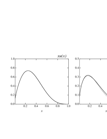
Figure 1: Unpolarized valence quark distribution functions of the proton at $Q^{2}=1\mbox{GeV}^{2}$. The $u$-quark distribution is depicted in the left figure, and $d$-quark in the right one. Our parametrizations are shown by the solid curves and CTEQ4LQ[14] by the dashed curves.

We also use the following distribution functions to get numerical results. The transverse momentum distributions for $y$ and $z$ components are assumed to be the Gaussian types as already introduced in eq. (2). The picked-up antiquark distribution function is taken to be $g_{2}^{sea}(x)\sim C(1-x)^{4}x^{-0.5}$ ($C$ is the constant number). Compared with the standard parametrization of the antiquark distribution of the proton[14], $g_{2}^{sea}(x)$ possibly involves high momentum components, because we assume that this antiquark distribution originates from the $q\bar{q}$ pair creation by the string breaking in the soft hadronization process. The resulting analyzing powers are insensitive to the variation of $g_{2}^{sea}$ and $G_{\pi}(x,y,z)$. For example, even if we take $g_{2}^{sea}\sim(1-x)^{6-8}$ adopted in ref. [7], the behavior of the analyzing power is almost unchanged. It may be possible to fix the picked-up antiquark distribution in order to reproduce the $x_{F}$ and $p_{T}$ dependence of the unpolarized cross section, and such a study is in progress[19].

Before we shall discuss the analyzing powers, let us consider the unpolarized cross section for $\pi^{+}$ and $\pi^{-}$ at large $x_{F}$ in the quark recombination model. Parameters of the model are already fixed to reproduce the data of the hyperon polarizations, which can be found in ref. [4]. In Fig.2 we show a ratio of $\pi^{+}$ to $\pi^{-}$ cross sections with experiments[20]. The calculation agrees with the data nicely. If we used the CTEQ4 or other standard parton distribution functions where $u/d\rightarrow\infty$ ($x\rightarrow 1$), this curve would blow up at $x_{F}\sim 1$, which seems to be inconsistent with the data.

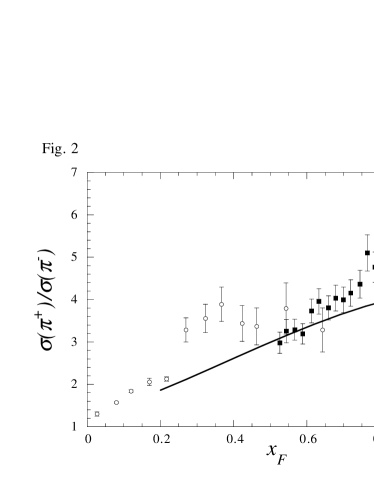
Figure 2: Ratio of the inclusive $\pi^{+}$ to $\pi^{-}$ production cross sections at $p_{T}=0.75\mbox{GeV}$. Experimental data are taken from ref. [20].

We finally show in Fig.3 spin asymmetries for pions with the experimental data at $p_{T}=0.75\mbox{GeV}$. Absolute magnitude of $A_{N}(\pi^{-})$ is almost the same as one of $A_{N}(\pi^{+})$, which reasonably reproduces the data. The asymmetry of $\pi^{0}$ is also in a good agreement. These results are understood by the following very simplified discussion. At $x_{F}\sim 1$, relative magnitudes of the analyzing powers in $\pi^{a}$ are intuitively given by ratios of spin-dependent to spin-independent distribution functions at $x\sim 1$,

$$A_{N}(\pi^{+}):A_{N}(\pi^{-}):A_{N}(\pi^{0})\sim\frac{\delta u(x\sim 1)}{u(x\sim 1)}:\frac{\delta d(x\sim 1)}{d(x\sim 1)}:\frac{\delta u(x\sim 1)+\delta d(x\sim 1)}{u(x\sim 1)+d(x\sim 1)}\;.$$

According to our procedure in eqs. (8,12), we employ a relation $u(x)=5d(x)$ and $\delta u(x)=u(x)$, $\delta d(x)=-d(x)$ at $x\sim 1$. Thus, it is easy to see,

$$A_{N}(\pi^{+}):A_{N}(\pi^{-}):A_{N}(\pi^{0})\sim 1:-1:\frac{2}{3}\hskip 28.45274pt\mbox{at }\hskip 8.5359ptx_{F}\sim 1\;,$$ (13)

which evidently accounts for essential features of the experiments shown in Fig.3. Also, our calculations reasonably describe the data on the pion analyzing powers of the polarized antiproton-proton scatttering[2].

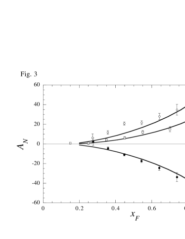
Figure 3: Analyzing powers of $\pi^{+}$, $\pi^{-}$ and $\pi^{0}$ from the transversely polarized proton with $p_{T}=0.75\mbox{GeV}$. Experimental data are depicted by the open circles, filled circles and open boxes for $\pi^{+}$, $\pi^{-}$ and $\pi^{0}$, respectively[2]. Our results are shown by the solid curves.

To be more realistic, true behavior of $u(x)/d(x)$ lies somewhere between the standard prametrization eq. (10) ($u(x)/d(x)\to\infty$) and the perturvative QCD motivated constraint eq. (12) ($u(x)/d(x)\to 5$). It is actually seen that the experimental data on the unpolarized cross section ratio $\sigma(\pi^{+})/\sigma(\pi^{-})\sim u(x)/d(x)$ is slightly larger than 5 obtained by the parametrization eq. (12). Anyways, the parametrization eq. (12) gives much better results for both the cross section ratio and the spin asymmetry. Therefore, we expect the perturbative QCD inspired distributions eq. (12) to be more reasonable as the valence quark distribution of the nucleon in this work. At the present, the experimental data of the analyzing power for $\pi^{0}$ are available at $x_{F}\leq 0.7$. Forthcoming data at much higher $x_{F}$ may provide some new constraints on the large-$x$ behavir of the quark distribution in the nucleon.

Analyzing powers in inclusive kaon production $\vec{p}+p\rightarrow K+X$ can be calculated in the same way. This model predicts asymmetries in $K^{-}$ and $\bar{K}^{0}$ vanish, because the proton does not contains (fast) valence $\bar{u}$ or $\bar{d}$ quarks. $K^{+}$ analyzing power is positive, whereas $K^{0}$ gives a negative asymmetry. We present the analying powers of $K^{+}$ and $K_{0}$ in Fig.4 with the kaon distribution[21]. Relative magnitude for large $x_{F}$ kaons is obtained as

$$A_{N}(K^{+}):A_{N}(K^{0})=1:-1\;\;.$$ (14)

Note that the SU(6) symmetry consideration leads to a result $A_{N}(K^{+}):A_{N}(K^{0})=2:-1$. This prediction will be tested in future experiments.

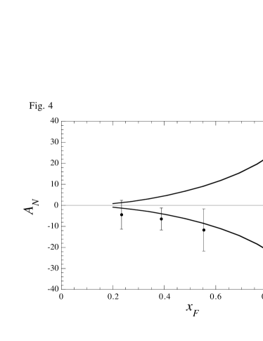
Figure 4: Analyzing powers of $K^{+}$ and $K^{0}$ with $p_{T}=0.75\mbox{GeV}$ are shown by the solid and dashed curves, respectively. Experimental data of $K^{0}_{s}$ are also shown by the filled circles.

We also calculate the case of inclusive $\rho$ meson production for polarizations and analyzing powers. Results strongly depend on the choice of the $\rho$ meson wave function, which will be published elsewhere[19].

In conclusion, we have studied the analyzing powers in inclusive pion productions $\vec{p}+p\rightarrow\pi^{a}+X$ at high $x_{F}$ in terms of the quark recombination model. We have particularly emphasized that the analyzing power is sensitive to the large Bjorken $x$ dependence of the spin distribution function in the nucleon. Calculations based on the SU(6) spin-flavor symmetry of the nucleon cannot describe relative magnitudes of analyzing powers in $\pi^{+}$, $\pi^{-}$ and $\pi^{0}$. However, once we take into account the realistic quark distribution functions which deviate from the SU(6) predictions at large Bjorken $x$, as suggested by the deep inelastic scattering and effective quark model calculations, resulting analyzing powers show reasonable agreement with the data. These results may indicate that the spin dependent inclusive hadron production at the high $x_{F}$ region, which are accessible at RHIC and HERA-N, is a complemental tool to probe the valence quark spin structure of the nucleon at large $x$.

Acknowledgments

K.S. would like to thank the COE program, which enables him to work out this project at RCNP.

References

-
[1]
G. Bunec et al., Phys. Rev. Lett. 36 (1976)
1113
Recent experimental references are found in ref. [4]. -
[2]
D.L. Adams et al., Phys. Lett. B264 (1991) 463
A. Bravar et al., Phys. Rev. Lett. 77 (1996) 2626
D.L. Adams et al., Z. Phys. C56 (1992) 181 - [3] T.A. DeGrand and H.I. Miettinen, Phys. Rev. D23 (1981) 1227, ibid D24 (1981) 2419, D31 (1985) 661(E)
- [4] Y. Yamamoto, K.-I. Kubo and H. Toki, Prog. Theor. Phys. 98 (1997) 95
-
[5]
B. Andersson, G. Gustafson and G. Ingelman, Phys.
Lett. B85 (1979) 417
J. Soffer and N.A. Tornqvist, Phys. Rev. Lett. 68 (1992) 907 -
[6]
C. Boros, L. Zuo-tang and M. Ta-chung, Phys. Rev. D51 (1995) 4867
M. Anselmino, M. Boglione and F. Murgia, Phys. Lett. B362 (1995) 164
S.M. Troshin and N.E. Tyurin, Phys. Rev. D54 (1996) 838
X. Artru, J. Czyzewski and H. Yabuki, Z. Phys. C73 (1997) 527
J. Qiu and G. Sterman, hep-ph/9806356
M. Anselmino and F. Murgia, hep-ph/9808426 -
[7]
K.P. Das and R.C. Hwa, Phys. Lett. B68 (1977) 459
E. Takasugi and X. Tata, Phys. Rev. D26 (1982) 120 - [8] T. Huang, B-Q. Ma and Q-X. Shen, Phys. Rev. D49 (1994) 1490
-
[9]
J.J. Aubert et al. (EMC), Nucl. Phys. B293
(1987) 740
A.C. Benvenuti et al. (BCDMS), Phys. Lett. B237 (1990) 599 -
[10]
P. Anthony et al. (SLAC E-142), Phys. Rev. D54
(1996) 6620
D. Adams et al. (SMC), Phys. Rev. D56 (1997) 5330
A. Airapetian et al. (HERMES), hep-ex/9807015 - [11] R.L. Jaffe and X. Ji, Nucl. Phys. B375 (1992) 527
- [12] J. Soffer, Phys. Rev. Lett. 74 (1995) 1992
- [13] K. Suzuki and T. Shigentani, Nucl. Phys. A626 (1997) 886
- [14] H.L. Lai et al., Phys. Rev. D55 (1997) 1280
- [15] A.D. Martin et al., Euro. Phys. J. C4 (1998) 463
- [16] W. Melnitchouk and A.W. Thomas, Phys. Lett. B377 (1996) 11
- [17] G.R. Farrar and D.R. Jackson, Phys. Rev. Lett. 35 (1975) 1416
- [18] U.K. Yang and A. Bodek, hep-ph/9809480
- [19] N. Nakajima, K. Suzuki, H. Toki, K.-I. Kubo, to be published
-
[20]
J.L. Bailly et al., Z. Phys. C35 (1987) 309
J. Singh et al., Nucl. Phys. B140 (1978) 189 - [21] T. Shigetani, K. Suzuki and H. Toki, Phys. Lett. B308 (1993) 383; Nucl. Phys. A579 (1994) 413