Abstract

The Wilsonian renormalization group (RG) method is applied to finite temperature systems for the study of non-perturbative methods in the field theory. We choose the $O(N)$ linear sigma model as the first step. Under the local potential approximation, we solve the Wilsonian RG equation as a non-linear partial differential equation numerically. The evolution of the domain is taken into account using the naive cut and extrapolation procedure. Our procedure is shown to yield the correct solution obtained by the auxiliary field method in the large $N$ limit. To introduce thermal effects, we consider two schemes. One in which the sum of the Matsubara frequencies are taken before the scale is introduced is found to give more physical results. We observe a second order phase transition in both the schemes. The critical exponents are calculated and are shown to agree with the results from lattice calculations.

1 Introduction

Non-perturbative aspects of the quantum field theory are very interesting and important. Study of low-energy hadron properties in QCD is an example that non-perturbative approaches are indispensable. We expect a phase transition at finite temperature which can be understood only non-perturbatively. Various non-perturbative approaches have been developed, such as the super-daisy summation of diagrams, the instanton approach, $1/N$ expansion, $\epsilon$ expansion and so on. The program, however, has not been accomplished yet. Under this circumstance, the method of the Wilsonian renormalization group (RG) equation[1, 2, 3] receives much attention[4, 5, 6, 7, 8, 9]. The idea is to include the quantum effects gradually from high energy in order to obtain a low-energy (Wilsonian) effective action. This RG equation is a non-linear evolution equation with respect to the scale $\Lambda$ in the functional theory space. While $\Lambda$ is lowered, various irrelevant operators are reproduced and finally we obtain the effective action in which all quantum effects are included. This process can be achieved non-perturbatively. The concept of the Wilsonian RG equation is common to various quantum field theories in the sense that it is model independent in contrast to the instanton or $1/N$ expansion approaches. A systematic approximation is also possible in the form of enlargement of the functional theory space step by step.

In spite of these advantages, there are still technical difficulties in application. It is not easy to obtain the physical quantities while it is very useful to see the phase structure and the critical phenomena. This difficulty is especially serious in the symmetry broken phase. In order to treat the bottom flatened effective potential, which is naturally required in the quantum system, one must prepare a suitable functional theory space. There is a dilemma that the expected potential is non-analytic while the RG equation is a partial differential equation which assumes the smoothness of the solution.

The aim of this paper is to challenge this dilemma. We here propose to solve the RG equation as a difference equation in the explicit scheme. In the symmetry broken phase, we set the domain in which the solutions is continuous, and the domain size is modified at each step of integration. This approach may sound too naive but we demonstrate the availability of such numerical treatment of the Wilsonian RG in physical applications.

For this purpose we concentrate on the $O(N)$ linear sigma model. This model is often studied in other non-perturbative methods and its physical application is also very interesting. It can describe not only the spontaneous symmetry breaking but also the symmetry restoration above a critical temperature. Especially, the $O(N=4)$ symmetric model is known to be equivalent to the chiral $SU_{L}(2)\times SU_{R}(2)$ effective theory of QCD, and is widely expected to describe the chiral phase transition in QCD.

In Sect.2, we present our formulation of the Wilsonian RG equation and the numerical method for solving the equation in the local potential approximation. We demonstrate that our method works very well for the large $N$ limit, for which the auxiliary field method yields the correct answer. We apply our method for $N=4$ and show that the symmetry breaking is well represented in our method.

In Sect.3, we apply our method to finite temperature $O(N)$ model. We employ the imaginary time formalism. When the sum of the Matsubara frequencies is considered, we realize two possible schemes of treating the scale dependence. One is to cut-off the sum according to the scale change and the other is to take the sum before the scale is introduced. These two schemes should give the same results provided that the initial scale $\Lambda_{0}$ is infinite. However, in practice we choose a finite $\Lambda_{0}$ and the two schemes give different results. We examine both of them and in the end show that the second scheme is more appropriate.

The results for the $O(N)$ sigma model are presented. We obtain the second order phase transition to the chiral restored phase in the above two schemes. It is shown that the four dimensional system near the critical temperature in the first scheme reduces to a three dimensional system at zero temperature. This indicates the first scheme corresponds to taking the high temperature limit even near the critical temperature. On the other hand, in the second scheme we obtain more physical results. The critical exponents are computed and are shown to agree very well to the results in the lattice calculation.

The conclusion is given in Sect.4.

2 Wilsonian RG Equation

The lagrangian of the $O(N)$ linear sigma model we consider here is given by

$${\cal L}:=\frac{1}{2}(\partial_{\mu}\phi)^{2}+\frac{\mu^{2}}{2}\phi^{2}+\frac{\lambda}{8N}(\phi^{2})^{2}$$ (1)

in the Euclidean notation $\mu=1,2,3$ and $4$. $\phi$ denotes the $N$ component column vector $\phi:=(\phi_{1},\phi_{2},\cdots,\phi_{N})^{T}$.

The Wilsonian RG equation with a sharp cut-off scheme is called Wegner–Houghton (WH) equation. The WH equation in the $O(N)$ linear sigma model is derived in Ref.[7] and is given by

$$-\Lambda\frac{d\Gamma_{\Lambda}}{d\Lambda}=\frac{\Lambda}{2}\int_{|p|=\Lambda}d^{D}p\left\{-{\rm Tr}{\rm Ln}\left(\frac{1}{\Lambda^{2}}\frac{\delta^{2}\Gamma_{\Lambda}}{\delta\phi_{p}\delta\phi_{-p}}\right)+\frac{\delta\Gamma_{\Lambda}}{\delta\phi_{p}}\left(\frac{\delta^{2}\Gamma_{\Lambda}}{\delta\phi_{p}\delta\phi_{-p}}\right)^{-1}\frac{\delta\Gamma_{\Lambda}}{\delta\phi_{-p}}\right\}$$ (2)

in $D$ dimensional space-time. $\Gamma_{\Lambda}[\phi]$ denotes a scale dependent effective action at the scale $\Lambda$ above which the quantum fluctuation is included. Thus at $\Lambda=0$ the scale dependent effective action agrees with the conventional effective action $\Gamma[\phi]$. The integral of r.h.s. is the shell ($|p|=\Lambda$) integral

$$\int_{|p|=\Lambda}d^{D}p:=\int\frac{d^{D}p}{(2\pi)^{D}}\delta(|p|-\Lambda).$$ (3)

The first and the second terms in r.h.s. of Eq.$(\ref{AEQ:H110412:2})$ give ring and dumbbell diagrams respectively. For a given initial condition $\Gamma_{\Lambda_{0}}[\phi]$ at the scale $\Lambda_{0}$, the effective action $\Gamma_{\Lambda}[\phi]$ at any scale $\Lambda$ is obtained by solving the WH equation. As the initial condition for Eq.$(\ref{AEQ:H110412:2})$ we assume that the effective action $\Gamma_{\Lambda}[\phi]$ reduces at high $\Lambda_{0}$ to the classical action $S[\phi]$.

In practice, to solve the equation $(\ref{AEQ:H110412:2})$, suitable approximation is necessary. We employ the local potential approximation (LPA) which assume the functional space as

$$\Gamma_{\Lambda}[\phi]=\int d^{D}x\left\{\frac{1}{2}(\partial_{\mu}\phi)^{2}+V_{\Lambda}(\phi)\right\}.$$ (4)

Under this approximation, the dumbbell diagram does not contribute and the WH equation reads

$$\frac{dV_{t}(x)}{dt}=\frac{A_{D}\Lambda^{D}}{2}\left\{(N-1)\ln\left(1+\frac{1}{\Lambda^{2}}\frac{1}{x}\frac{\partial V_{t}}{\partial x}\right)+\ln\left(1+\frac{1}{\Lambda^{2}}\frac{\partial^{2}V_{t}}{\partial x^{2}}\right)\right\}$$ (5)

where $\Lambda:=\Lambda_{0}\exp(-t)$, $x:=\sqrt{\phi^{2}}$,

$$A_{D}:=\frac{\pi^{-D/2}2^{1-D}}{\Gamma(D/2)}$$ (6)

and $V_{t}(x)$ is a scale dependent effective potential.

We solve this equation numerically as a difference equation in the explicit scheme

$$\frac{V^{j+1}_{i}-V^{j}_{i}}{\Delta t}=\frac{A_{D}\Lambda^{D}_{j}}{2}\Bigg{\{}(N-1)\ln\left(1+\frac{1}{\Lambda^{2}_{j}}\frac{1}{x_{i}}\frac{V^{j}_{i+1}-V^{j}_{i-1}}{2\Delta x}\right)$$ (7)

$${}+\ln\left(1+\frac{1}{\Lambda_{j}^{2}}\frac{V^{j}_{i+1}-2V^{j}_{i}+V^{j}_{i-1}}{(\Delta x)^{2}}\right)\Bigg{\}}$$

where $t_{j}:=j\Delta t$, $\Lambda_{j}:=\Lambda_{0}\exp(-t_{j})$, $x_{i}:=i\Delta x$ and $V^{j}_{i}:=V_{t_{j}}(x_{i})$ with $j=0,\cdots,j_{\rm max}$ and $i=0,\cdots,i_{\rm max}$. This explicit scheme suggests us that a large $j_{\rm max}$ is necessary for a large $i_{\rm max}$. Furthermore there is a subtle problem in solving Eq.$(\ref{AEQ:H110414:3})$, that is , we have to specify the domain ${\cal D}$ of $x$. In the broken phase, the field variable can not take all the values because the field variable $\phi$ is not an analytic function of the source $J$ around the origin $\phi=0$. Numerically the arguments of logarithm become zero or negative for $x$ with $|x|\leq\,^{\exists}\!a$ at some $t_{j}$. In such cases, we obtain the effective potential at $t_{j+1}$ only by the information of the region $x$ with $|x|>a$. Thus, we consider the domain ${\cal D}=\{x\,|\,|x|>a\}$. On the other hand, when the arguments of the logarithm grows up from zero at the end point $x=a$ of the domain ${\cal D}$ at $t_{j}$, we extrapolate the arguments as a smooth function of $x$ using vicinal four points by

$$f(x_{m-1}) \approx f(x_{m})-f^{\prime}(x_{m})\Delta x$$ (8)

$$\approx f(x_{m})-\left(f^{\prime}(x_{m+1})-f^{\prime\prime}(x_{m+1})\Delta x\right)\Delta x$$

$$\approx f(x_{m})-\left(\frac{f(x_{m+2})-f(x_{m})}{2\Delta x}-\frac{f(x_{m+2})-2f(x_{m+1})+f(x_{m})}{\Delta x}\right)\Delta x$$

where $x_{m}$ is the nearest neighbor to $a$ and we enlarge the domain ${\cal D}$ at $t_{j+1}$. The numerical result seems to be almost independent of the extrapolation procedure if we take sufficiently large $i_{\rm max}$ (and $j_{\rm max}$).

We choose the mass unit as $\Lambda_{0}$ so that $\Lambda_{0}=1$, concentrate on $D=4$, and set $\hat{\mu^{2}}=\mu^{2}/\Lambda_{0}^{2}=-0.6$ and $\lambda/8N=4$ so as to bring out the spontaneous symmetry breaking. We employ the numerical parameters $i_{\rm max}=400$ and $j_{\rm max}=10^{5}$.

First we consider the large $N$ limit, where the LPA WH equation $(\ref{AEQ:H110414:2})$ reduces to

$$\frac{dV_{t}(x)}{dt}=\frac{A_{D}\Lambda^{D}}{2}N\ln\left(1+\frac{1}{\Lambda^{2}}\frac{1}{x}\frac{\partial V_{t}}{\partial x}\right).$$ (9)

Eq.$(\ref{AEQ:H110414:4})$ is solved for the initial condition

$$V_{t=0}(x)=\frac{\mu^{2}}{2}x^{2}+\frac{\lambda}{8N}x^{4}.$$ (10)

The result is shown in Fig.1.

Figure 1: The solutions of the Wilsonian RG equation for the large $N$ limit. The curves correspond to $t=0.0,0.2,0.5,1.0,9.9$ from bottom to top respectively.

For $t=0.0\sim 0.5$, the effective potential becomes gradually flat as the quantum correction is included. This resembles the lattice result in Ref.[10]. For $t>0.5$, however, the effective potential becomes complex from the inside and the Domain develops. As stated above, we do not use the values of such complex region in computing the next step. It is plausible that this region should be perfectly flattened as is indicated by the study at $t\to\infty$ in Ref.[10]. It should be noted that the point of the potential minimum, which gives the vacuum expectation value of $\phi$, and the end point of the domain become close to each other. Finally, at $t\to\infty$, these two points coincide and the effective potential defined conventionally is obtained.

It is well-known that the exact effective potential can be obtained using the auxiliary field method in the large $N$ limit [11, 12]. As a result, the scale dependent form of the effective potential is given by

$$V_{t}(x)=V_{t}(x,s)=\frac{1}{2}x^{2}s-\frac{N}{2\lambda}s^{2}+\frac{N\mu^{2}}{\lambda}s+\frac{N}{2}\int_{\Lambda}^{\Lambda_{0}}\frac{d^{4}k}{(2\pi)^{4}}\ln(k^{2}+s)$$ (11)

where the auxiliary field $s$ is a function of $x$ and is given by a solution of the saddle point condition

$$\frac{\partial V_{t}(x,s)}{\partial s}=0.$$ (12)

It is easy to see that Eq.$(\ref{AEQ:H110414:5})$ is the solution of Eq.$(\ref{AEQ:H110414:4})$ with the initial condition $(\ref{AEQ:H110512:1})$ [13]. We find that our numerical solutions in Fig.1 agree almost completely to the analytic solution Eq.$(\ref{AEQ:H110414:5})$.

In plotting Fig.1, we only take the region of $\phi$ where $V_{t}(x)$ is real. In fact, for each $t$ there is a critical value of $x_{c}(t)=|\phi_{c}(t)|$ below which the solution of Eq.$(\ref{AEQ:H110414:6})$ becomes complex. In the present case,

$$x_{c}(t=\infty)=2N\min_{s}\left\{\frac{s-\mu^{2}}{\lambda}-\frac{A_{D}}{4}\left(\Lambda_{0}^{2}-s\ln\frac{\Lambda_{0}^{2}+s}{s}\right)\right\}$$ (13)

This phenomenon occurs where the $O(N)$ symmetry is spontaneously broken and the system generates a non-zero vacuum expectation value of $\phi$. The magnitude of the vacuum condensate of $\phi$ is given by the critical value at $t\to\infty$ or $\Lambda\to 0$.

Next we consider the finite $N$ case. The O(4) result is shown in Fig.2. Again the complex region appears. One sees that the qualitative behavior of the effective potential is quite similar to that for the large $N$ limit and that the calculation supports the spontaneous symmetry breaking. The evolution of the domain by the scale is shown in Fig.3. We see that the curves are monotonically increasing and saturate at about $t\sim 5$ ($\Lambda\sim 0.007$).

Figure 2: Solution of the Wilsonian RG equation for $N=4$. The curves correspond to $t=0.0,0.5,10$ from bottom to top respectively.

Figure 3: The end points $a$ of the domain v.s. the scale variable $t$. The curves correspond to the temperature $T=0.0,0.1,0.15$ from top to bottom respectively.

3 Finite Temperature

The introduction of the thermal effects is discussed in many text books [14]. We use the imaginary time formalism in which the loop momentum integration is replaced by the sum of the Matsubara frequencies as

$$\int\frac{d^{D}p}{(2\pi)^{D}}\Longrightarrow T\sum_{n}\int\frac{d^{D-1}p}{(2\pi)^{D-1}},\quad p_{0}=2n\pi T$$ (14)

where $T$ denotes the temperature. The system is now controlled by the new dimensional parameter $T$. There are some candidates how to extend the evolution equation in order to include the effect of $T$. We consider the following two schemes within the local potential approximation.

Scheme I

Firstly we consider the 4-dimensional spherical cut-off scheme. For $T=0$, the formula

$$\Lambda\frac{1}{\delta\Lambda}\int_{\Lambda-\delta\Lambda\leq p\leq\Lambda}\frac{d^{D}p}{(2\pi)^{D}}=\Lambda\frac{1}{\delta\Lambda}\int_{\Lambda-\delta\Lambda}^{\Lambda}dp\,p^{D-1}\int\frac{d\Omega_{p}}{(2\pi)^{D}}$$ (15)

$$\stackrel{{\scriptstyle\delta\Lambda\to 0}}{{\to}} \Lambda^{D}\int\frac{d\Omega_{p}}{(2\pi)^{D}}=\int_{|p|=\Lambda}dp.$$

is used in the derivation of the WH equation $(\ref{AEQ:H110412:2})$. If a function $f(p^{2})$ depends only on $p^{2}$, then Eq.$(\ref{AEQ:H110414:8})$ reduces to

$$\Lambda\frac{1}{\delta\Lambda}\int_{\Lambda-\delta\Lambda\leq p\leq\Lambda}\frac{d^{D}p}{(2\pi)^{D}}f(p^{2})\stackrel{{\scriptstyle\delta\Lambda\to 0}}{{\to}}\Lambda^{D}A_{D}f(\Lambda^{2})$$ (16)

which is used as the prefactor in r.h.s. of Eq.$(\ref{AEQ:H110414:2})$. Even at finite temperature, the integrand is still $f(p^{2})$ within LPA and therefore the shell integration can be performed as

$$\Lambda\frac{1}{\delta\Lambda}\frac{1}{\beta}\sum\int_{\Lambda-\delta\Lambda\leq|p|\leq\Lambda}\frac{d^{D-1}p}{(2\pi)^{D-1}}f(p^{2})$$ (17)

$$= \frac{\Lambda}{\delta\Lambda}A_{D-1}\frac{1}{\beta}\sum\int_{\Lambda-\delta\Lambda\leq\sqrt{(2\pi n/\beta)^{2}+p_{r}^{2}}\leq\Lambda}dp_{r}p_{r}^{D-2}f\left(\left(\frac{2\pi n}{\beta}\right)^{2}+p_{r}^{2}\right)$$

$$= \frac{\Lambda}{\delta\Lambda}A_{D-1}\frac{1}{\beta}\sum_{|n|\leq\Lambda\beta/(2\pi)}\int_{\sqrt{(\Lambda-\delta\Lambda)^{2}-(2\pi n/\beta)^{2}}}^{\sqrt{\Lambda^{2}-(2\pi n/\beta)^{2}}}dp_{r}p_{r}^{D-2}f\left(\left(\frac{2\pi n}{\beta}\right)^{2}+p_{r}^{2}\right)$$

$$\stackrel{{\scriptstyle\delta\Lambda\to 0}}{{\to}} \Lambda^{D-1}A_{D-1}\frac{1}{\beta}\sum_{|n|\leq\Lambda\beta/(2\pi)}\left(1-\left(\frac{2\pi n}{\Lambda\beta}\right)^{2}\right)^{\frac{D-3}{2}}f(\Lambda^{2})$$

where $\beta:=1/T$. Comparing Eq.$(\ref{AEQ:H110414:9})$ and Eq.$(\ref{AEQ:H110414:10})$, we conclude that the thermal effect is taken into account by replacing the prefactor of r.h.s. of Eq.$(\ref{AEQ:H110414:2})$,

$$A_{D}\Lambda^{D}\Longrightarrow A_{D-1}\frac{\Lambda^{D-1}}{\beta}\sum_{|n|\leq\Lambda\beta/(2\pi)}\left(1-\left(\frac{2\pi n}{\Lambda\beta}\right)\right)^{\frac{D-3}{2}}.$$ (18)

Finally, we obtain the WH equation in the scheme I,

$$\frac{dV_{t}(x)}{dt}=\frac{A_{D-1}\Lambda^{D-1}}{2\beta}\sum_{|n|\leq\Lambda\beta/(2\pi)}\left(1-\left(\frac{2\pi n}{\Lambda\beta}\right)\right)^{\frac{D-3}{2}}$$ (19)

$${}\times\left\{(N-1)\ln\left(1+\frac{1}{\Lambda^{2}}\frac{1}{x}\frac{\partial V_{t}}{\partial x}\right)+\ln\left(1+\frac{1}{\Lambda^{2}}\frac{\partial^{2}V_{t}}{\partial x^{2}}\right)\right\}.$$

Here it should be noted that the thermal loop contribution is summed up only for $|n|\leq\Lambda_{0}\beta/2\pi$ in the scheme I. For $\Lambda_{0}\to\infty$, this scheme provides the full thermal loop correction, while for relatively small $\Lambda_{0}$, the summation is limited to low $|n|$ especially at high temperature. Indeed, we will see later that the limited summation gives a fluctuation in the effective potential. In order to avoid this difficulty, we next consider the second scheme.

Scheme II

We consider the scheme in which the cut-off is introduced after the separation of the quantum and thermal effects. In this scheme, therefore, we perform the summation of all Matsubara frequencies.

For simplicity, we focus only on LPA. Suppose that the effective potential $V_{t}(\phi)$ is given at the scale $t$. Then the effective potential $V_{t+\Delta t}(\phi)$ is given by

$$V_{t+\Delta t}(\phi) = V_{t}(\phi)+\frac{1}{2\beta}\sum\int\frac{d^{D-1}k}{(2\pi)^{D-1}}\ln\det\left[k^{2}+\frac{\delta^{2}V_{t}(\phi)}{\delta\phi^{T}\phi}\right]$$ (20)

$${}+\mbox{ \vspace*{14pt} (2-loop and higher loop contributions) }$$

where the integral is performed between $t$ and $t+\Delta t$. To specify the cut-off scheme we use the formula

$$\frac{1}{\beta}\sum_{n}\int\frac{d^{D-1}k}{(2\pi)^{D-1}}\ln((2n\pi T)^{2}+\vec{k}^{2}+M^{2})=\int\frac{d^{D}k}{(2\pi)^{D}}\ln(k^{2}+M^{2})$$ (21)

$${}+\frac{2}{\beta}\int\frac{d^{D-1}k}{(2\pi)^{D-1}}\ln(1-\exp(-\beta\sqrt{k^{2}+M^{2}}))$$

$$= \int_{\Lambda=0}^{\Lambda=\infty}d\Lambda\left\{\frac{A_{D}\Lambda^{D-1}}{2}\ln(\Lambda^{2}+M^{2})+\frac{A_{D-1}\Lambda^{D-2}}{\beta}\ln(1-\exp(-\beta\sqrt{\Lambda^{2}+M^{2}}))\right\}$$

where $\beta=1/T$ and $M^{2}$ is an arbitrary constant. In r.h.s. the quantum and thermal effects are separated. Thus we introduce a sharp cut-off of $\Lambda$ in Eq.$(\ref{AEQ:H110414:13})$. Similar procedure can be performed for the 2-loop and higher loop contributions. The cut-off is introduced so that in the quantum correction part the radial mode in the 4-dimensional integration is cut-off, while in the thermal correction part radial mode in the 3-dimensional integration which is left after the summation or the integration with respect to $k_{0}$ is cut-off. Taking the limit $\Delta t\to 0$ in Eq.$(\ref{AEQ:H110414:12})$, the 2-loop and higher loop contributions vanish. Therefore we conclude that the thermal effect is included by adding

$$\frac{A_{D-1}\Lambda^{D-1}}{\beta}\Bigg{\{}(N-1)\ln\left(1-\exp\left(-\beta\sqrt{\Lambda^{2}+\frac{1}{x}\frac{\partial V_{t}}{\partial x}}\right)\right)$$ (22)

$${}+\ln\left(1-\exp\left(-\beta\sqrt{\Lambda^{2}+\frac{\partial^{2}V_{t}}{\partial x^{2}}}\right)\right)\Bigg{\}}$$

to r.h.s. of Eq.$(\ref{AEQ:H110414:2})$.

Finally we obtain the WH equation in the scheme II.

$$\frac{dV_{t}(x)}{dt}=\frac{A_{D}\Lambda^{D}}{2}\left\{(N-1)\ln\left(1+\frac{1}{\Lambda^{2}}\frac{1}{x}\frac{\partial V_{t}}{\partial x}\right)+\ln\left(1+\frac{1}{\Lambda^{2}}\frac{\partial^{2}V_{t}}{\partial x^{2}}\right)\right\}$$ (23)

$${}+\frac{A_{D-1}\Lambda^{D-1}}{\beta}\Bigg{\{}(N-1)\ln\left(1-\exp\left(-\beta\sqrt{\Lambda^{2}+\frac{1}{x}\frac{\partial V_{t}}{\partial x}}\right)\right)$$

$${}+\ln\left(1-\exp\left(-\beta\sqrt{\Lambda^{2}+\frac{\partial^{2}V_{t}}{\partial x^{2}}}\right)\right)\Bigg{\}}.$$

It is noted that neglecting the quantum effects (the first term in r.h.s.), this evolution equation coincides with the thermal RG equation in Ref.[15], which is derived in the real time formalism [16], up to an additional step function.

In these two schemes, both Eqs.$(\ref{AEQ:H110414:15})$ and $(\ref{AEQ:H110414:16})$ reduce to the zero temperature formula Eq.$(\ref{AEQ:H110414:2})$ in the limit $T\to 0$ and they reduce in the limit $T\to\infty$ to the effective $D-1$ dimensional form

$$\frac{dV_{t}(x)}{dt}=\frac{A_{D-1}\Lambda^{D-1}}{2\beta}\left\{(N-1)\ln\left(1+\frac{1}{\Lambda^{2}}\frac{1}{x}\frac{\partial V_{t}}{\partial x}\right)+\ln\left(1+\frac{1}{\Lambda^{2}}\frac{\partial^{2}V_{t}}{\partial x^{2}}\right)\right\}.$$ (24)

The difference between the two schemes come from the cut-off procedure. Taking $\Lambda_{0}\to\infty$, their effective potentials at $\Lambda=0$ coincide. In practice, however, we neglect the thermal effect above $\Lambda_{0}$ in the first scheme and assume that $\Gamma_{\Lambda_{0}}$ equals to the zero temperature action. Thus the two schemes give different results for finite $\Lambda_{0}$.

In the scheme I, the numerical results are as follows. Fig.4 shows the vacuum expectation value of $\phi$ as a function of the temperature $T$ in the large $N$ limit of Eq.$(\ref{AEQ:H110414:15})$. Fig.5 shows the same quantity calculated by using the auxiliary field method. As these two curves agree well, we conclude that our numerical approach is appropriate. The result for $N=4$ is given in Fig.6. In these graphs, one sees unnatural steps. They come from the summation in Eq.$(\ref{AEQ:H110414:15})$. The summation is limited to a few terms when $T$ becomes comparable to $\Lambda_{0}/2\pi$ ($\approx 150$ [MeV] for $\Lambda_{0}=1$ [GeV]). As the vacuum expectation value is sensitive to the number of the summation in the initial condition, there appear unnatural steps seen in the results. Since the critical temperature $T_{c}=0.185$ shown in Fig.4 is larger than $\Lambda_{0}/2\pi$, the phase transition in this scheme I is controlled by the high temperature formula Eq.$(\ref{AEQ:H110415:1})$. At low temperature, we do not see such steps and the results agree very well with those obtained in our second scheme.

In Fig.7, we plot $\log(\phi)$ as a function of $\log(T_{c}-T)$, where $T_{c}$ denotes the critical temperature. After fitting the curve to the linear function using the least square method, we obtain the critical exponent $\beta=0.448$, defined by

$$\phi\propto|T_{c}-T|^{\beta}.$$ (25)

We also obtain the critical exponent $\delta=3.80$ from Fig.8, where $\delta$ is defined by

$$V\propto|\phi|^{\delta+1}$$ (26)

at $T=T_{c}$. In the same way we obtain the critical exponent $\gamma=1.43$ from Fig.9, where $\gamma$ is defined by

$$\frac{d^{2}V}{d\phi^{2}}\propto|T_{c}-T|^{\gamma}.$$ (27)

These results are summarized in Table 1. From Eqs.$(\ref{AEQ:H110510:1})$-$(\ref{AEQ:H110517:2})$, we obtain a scaling relation among the exponents,

$$\gamma=\beta(\delta-1).$$ (28)

Our numerical results yield $\beta(\delta-1)/\gamma=0.877$, which is not far from $1$.

Figure 4: Temperature dependence of the condensation $\phi$ as a function of temperature $T$ in the scheme I for the large $N$ limit.

Figure 5: The same as Fig.4 obtained in the auxiliary field method.

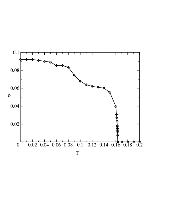
Figure 6: The temperature dependence of the condensation $\phi$ in the scheme I for $N=4$.

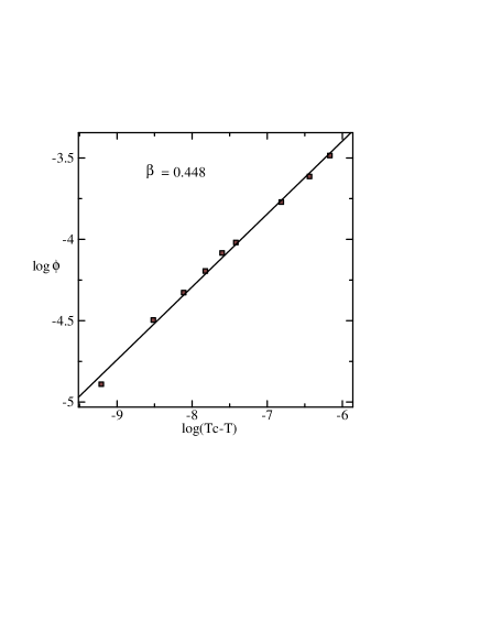
Figure 7: The critical exponent $\beta$ for the result of the Wilsonian RG method for $N=4$ in the scheme I.

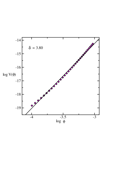
Figure 8: The critical exponent $\delta$ for $N=4$ in the scheme I.

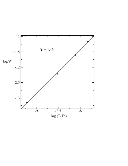
Figure 9: The critical exponent $\gamma$ for $N=4$ in the scheme I.

Numerical results of the scheme II are shown in Figs.10-12 and Table 1. In this scheme the summation of the infinite number of the Matsubara frequencies is performed. Therefore in the scheme II the unnatural steps seen in the scheme I do not appear. These curves again show the second order chiral phase transition. We estimate the critical exponent $\beta=0.384$ from Fig.13. This value agrees with the value $0.384$ obtained by the Monte-Calro calculation in Ref.[17], where the $O(N)$ Heisenberg model in three dimension is used. We also obtain the critical exponent $\delta=4.70$ from Fig.14. The value given in Ref.[17] is $\delta=4.85$. In the same way, we obtain the critical exponent $\gamma=1.38$ from Fig.15. The value in Ref.[17] is $\gamma=1.48$ which is also close to ours. These critical exponents satisfy the scaling relation very well, giving $\beta(\delta-1)/\gamma=1.03$.

	$\beta$	$\delta$	$\gamma$	$\beta(\delta-1)/\gamma$
Scheme I	$0.448$	$3.80$	$1.43$	$0.877$
Scheme II	$0.384$	$4.70$	$1.38$	$1.03$
Monte-Calro[17]	$0.384$	$4.85$	$1.48$	—

Table 1: Critical Exponents

Figure 10: The temperature dependence of the condensation $\phi$ in the scheme II for the large $N$ limit.

Figure 11: The same as Fig.10 in the auxiliary field method.

Figure 12: The temperature dependence of the condensation $\phi$ in the scheme II for $N=4$.

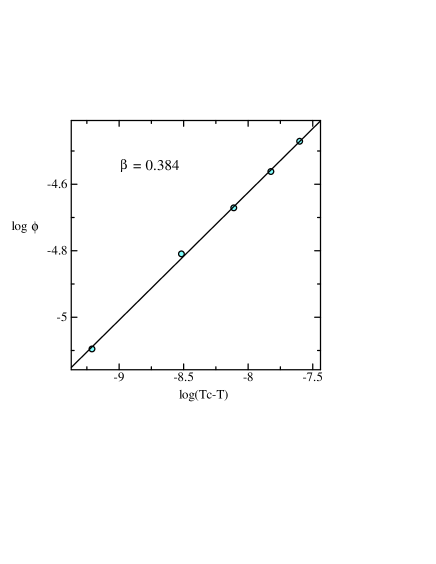
Figure 13: The critical exponent $\beta$ for $N=4$ in the scheme II.

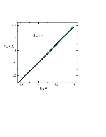
Figure 14: The critical exponent $\delta$ for $N=4$ in the scheme II.

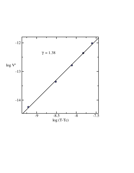
Figure 15: The critical exponent $\gamma$ for $N=4$ in the scheme II.

4 Conclusion

We have applied the Wilsonian RG method as the non-perturbative calculation method in the field theory to the $O(N)$ linear sigma model and calculated the low energy effective potential in the local potential approximation. We have introduced a numerical recipe to define the domain for the effective potential and have tested the method in the large $N$ limit. The results coincide with the solutions obtained by the auxiliary field method very well. This means that our numerical treatment of the Wilsonian RG equation is sufficiently good in this situation. We have also shown that the $N=4$ effective potential behaves similarly as those in the large $N$ limit.

We have applied our approach to the finite temperature system to see the chiral restoration phase transition. We have employed the imaginary time formulation using the sum of the Matsubara frequencies. When we take the sum of the Matsubara frequencies, we consider two schemes. In the scheme I, we use the 4-dimensional spherical cut-off. Then the sum of the Matsubara frequencies is also limited accordingly. In the scheme II, we separate the quantum and thermal effects, before the momentum integral is cut-off. These two schemes should agree with each other if the initial $\Lambda_{0}$ is infinite. In the scheme I, however, we assume that the thermal effect above $\Lambda_{0}$ is negligible and $\Gamma_{\Lambda_{0}}$ equals to the zero temperature action. Thus the two schemes give different results for finite $\Lambda_{0}$. Both of them show the second order phase transition. But the results of the scheme I have unnatural steps. These steps arise in the course of transfer from the four dimensional system to the three dimensional one at high temperature. On the other hand we have found that the scheme II gives more natural and physical results. Especially, the critical exponents in the scheme II are very close to that of Monte-Calro calculation.

Our aim has been to check whether our numerical method can be reliably applied to the Wilsonian renormalization group equation. We have demonstrated that it works very well in the $O(N)$ linear sigma model. It has been shown also that the method can be applied to finite temperature system. This is the first step of our approach to more complicated systems including fermions and gauge fields. The Wilsonian RG method provides us with a powerful tool to study non-perturbative features of low energy effective theories. As a next step, for instance, this approach may be able to judge whether certain effective model is consistent with QCD by comparing the solution of the Wilsonian RG equation for the effective model and the result of the lattice QCD.

References

- [1] F. J. Wegner and A. Houghton, Phys. Rev. A8 (1973) 401.
- [2] K. Wilson and J. Kogut, Phys. Rep. 12 (1974) 75.
- [3] J. Polchinski, Nucl. Phys. B231 (1984) 269.
- [4] T. R. Morris, Int. J. Mod. Phys. A9 (1994) 2411.
- [5] U. Ellwanger and C. Wetterich, Nucl. Phys. B423 (1994) 137.
- [6] J. Adams, J. Berges, S. Bornholdt, F. Freire, N. Tetradis and C. Wetterich, Mod. Phys. Lett. A10 (1995) 2367.
- [7] K.-I. Aoki, K. Morikawa, W. Souma, J.-I. Sumi and H. Terao, Prog. Theor. Phys. 95 (1996) 409.
- [8] K.-I. Aoki, K. Morikawa, J.-I. Sumi, H. Terao and M. Tomoyose, Prog. Theor. Phys. 97 (1997) 479.
- [9] J. Berges, D. U. Jungnickel and C. Wetterich, Phys. Rev. D59 (1999) 0304010 (hep-ph/9705474).
- [10] H. Mukaida and Y. Shimada, Nucl. Phys. B479 (1996) 663.
- [11] J. M. Cornwall, R. Jackiw and H. Politzer, Phys. Rev. D 10 (1974) 2491.
- [12] M. Kobayashi and T. Kugo, Prog. Theor. Phys. 54 (1975) 1537.
- [13] K.-I. Aoki, K. Morikawa, W. Souma, J.-I. Sumi and H. Terao, Prog. Theor. Phys. 99 (1998) 451.
- [14] J. I. Kupusta, Finite Temperature Field Theory, (Cambridge University Press, 1989); M. Le Bellac, Thermal Field Theory, (Cambridge University Press, 1996); A. Das, Finite Temperature Field Theory, (World Scientific, 1997)
- [15] B. Bergerhoff and J. Reingruber, hep-ph/9809251.
- [16] B. Bergerhoff, Phys. Lett. B437 (1998) 381.
- [17] K. Kanaya and S. Kaya, Phys. Rev. D51 (1995) 2404.