Abstract

The cross section for two bosonic D0-branes is calculated in limit $\alpha^{\prime}\rightarrow 0$. It is found that the cross section shows Regge behavior.

1 Introduction

The idea of string theoretic description of gauge theories is an old idea [1] [2]. Despite of the years that passed on this idea, it is also activating different researches in theoretical physics [3][4][5][6].

On the other hand, in the last few years our understanding about string theory is changed dramatically; a stream which is called usually ”second string revolution” [7]. The scope of this stream is presentation of a unified string theory as a fundamental theory of the known interactions. One of the most applicable tools in the above program are D$p$-branes [8, 9]. It is conjectured, and confirmed by various tests, that these objects can be considered as a perturbative representation of nonperturbative charged solutions of the low energy of string theories.

It has been known for long time that hadron-hadron scattering processes have two different behaviors depending on the amount of the momentum transfer [10]. At large momentum transfer interactions appear as interactions between the hadron constituents, partons or quarks, and some qualitative similarities to electron-hadron scattering emerge. At high energies and small momentum transfer Regge trajectories are exchanged, the same which was the first motivation for the stringy picture of strong interaction. Besides the good fitting between Regge trajectories and the mass of strong bound-states has remained unexplained yet [1, 11] .

Deducing the above observations from a unified picture is the challenge of theoretical physics and it is tempting to search for the application of the recent string theoretic progresses in this area. In this way one may find D$p$-branes good tools to take their dynamics as a proper effective theory for the bound-states of quarks and QCD-strings (QCD Electric Fluxes) between them. The conventional string theory is believed to have relevant physics at Planck scale and beyond. To use the string theory tools for QCD-strings one should replace the parameters with those which are important in QCD. The case is somehow similar to the variation from early days of string theory as the theory of strong interaction to string theory as the theory of gravity. Pushing this idea in [12] the potential between two D0-branes at rest was calculated and the result appeared in good agreement with those come from phenomenology for quarks [13]. Here we concern the scattering problem. Based on the results of [14] we calculate the cross section for two bosonic D0-branes. It is found that the cross section shows the Regge behavior. This behavior has been used some years ago to fit the hadron-hadron total cross section data successfully [15, 16] (see also [17, 18] for other recent application of this behavior). Also the obtained cross section exhibits a rich Polology which can be corresponded with Regge poles.

2 On D-Branes

D$p$-branes are $p$ dimensional objects which are defined as (hyper)surfaces which can trap the ends of strings [9]. One of the most interesting aspects of D-brane dynamics appear in their coincident limit. In the case of coinciding $N$ D$p$-branes in a (super)string theory, their dynamics are captured by a dimensionally reduced $U(N)$ (S)YM theory to $p+1$ dimensions of D$p$-brane world-volume [19, 9, 20].

In case of D0-branes $p=0$, the above dynamics reduces to quantum mechanics of matrices, because only time exists in the world-line. The bosonic part of the corresponding Lagrangian is [22]

$$L=m_{0}{\rm Tr}\;\biggl{(}{\frac{1}{2}}D_{t}X_{i}^{2}+\frac{1}{4(2\pi\alpha^{\prime})^{2}}[X_{i},X_{j}]^{2}\biggl{)},i,j=1,\cdot\cdot\cdot,d,$$ (1)

where $\frac{1}{2\pi\alpha^{\prime}}$ and $m_{0}=(\sqrt{\alpha^{\prime}}g_{s})^{-1}$ are the string tension and the mass of D0-branes respectively. Here $D_{t}=\partial_{t}-iA_{0}$ acts as covariant derivative in the 0+1 dimensional gauge theory. For $N$ D0-branes $X$’s are in adjoint representation of $U(N)$ and have the usual expansion $X_{i}=x_{ia}T_{a}$, $a=1,\cdot\cdot\cdot N^{2}$.

In fact (1) is the result of the truncation of the string theory calculations in the so-called ”gauge theory limit” defined by

$$g_{s} \rightarrow 0,$$

$$l_{s} \rightarrow 0,$$

$$\frac{v}{l_{s}^{2}} = {\rm fixed},$$

$$\frac{b}{l_{s}^{2}} = {\rm fixed},$$ (2)

which $v$ and $b$ are the velocities and distances relevant to the problem and $l_{s}=\sqrt{\alpha^{\prime}}$ is the string length.

Firstly let us search for D0-branes in the above Lagrangian:
For each direction $i$ there are $N^{2}$ variables and not $N$ which one expects for $N$ particles. Although there is an ansatz for the equations of motion which restricts the $U(N)$ basis to its $N$ dimensional Cartan subalgebra. This ansatz causes vanishing the potential and one finds the equations of motion for $N$ free particles. In this case the $U(N)$ symmetry is broken to $U(1)^{N}$ and the interpretation of $N$ remaining variables as the classical (relative) positions of $N$ particles is meaningful. The center of mass of D0-branes is represented by the trace of the $X$ matrices.

In the case of unbroken gauge symmetry, the $N^{2}-N$ non-Cartan elements have a stringy interpretation, governing the dynamics of low lying oscillations of strings stretched between D0-branes. Although the gauge transformations mix the entries of matrices and the interpretation of positions for D0-branes remains obscure [21], but even in this case the center of mass is meaningful. So the ambiguity about positions only comes back to the relative positions of D0-branes.

Let us concentrate on the limit $\alpha^{\prime}\rightarrow 0$. In this limit to have a finite energy one has

$$[X_{i},X_{j}]=0,\;\;\;\forall\;i,j,$$ (3)

and consequently vanishing the potential term in the action. So D0-branes do not interact and the action reduces to the action of $N$ free particles

$$S=\int dt\sum_{a=1}^{N}{\frac{1}{2}}m_{0}\dot{x}_{a}^{2}.$$ (4)

But the above observation fails in the times which D0-branes arrive each other. When two D0-branes come very near each other two eigenvalues of $X_{i}$ matrices will become approximately equal and this make the possibility that the corresponding off-diagonal elements take non-zero values. In fact this is the same story of gauge symmetry restoration. In summary one may deduce that in the limit $\alpha^{\prime}\rightarrow 0$ D0-branes do not interact with each other except for when they coincide.

In the coincident limit the dynamics is complicated. The matrix position may be taken as:

$$X_{i}=\left(\matrix{x_{i}&Y_{i}\cr Y_{i}^{*}&-x_{i}}\right),$$ (5)

where $Y^{*}$ is the complex conjugate of $Y$. By inserting this matrix in the Lagrangian one obtains:

$$S=\int dt{\frac{1}{2}}\bigg{(}(2m_{0})\dot{X_{i}}^{2}+m_{0}\dot{Y}_{i}\dot{Y}_{i}^{*}-m_{0}\frac{1}{4(2\pi\alpha^{\prime})^{2}}(1-\cos^{2}\theta)x_{j}^{2}Y_{i}Y_{i}^{*}+m_{0}\dot{x}_{j}^{2}+O(Y^{3})\bigg{)},$$ (6)

with $X$ for the center of mass and $\theta$ is the angle between $\vec{x}$ and the complex vector $\vec{Y}$. As is apparent in the limit $\alpha^{\prime}\rightarrow 0$ which is in our direct interest the $x$ element can not take large values and have a small range of variation. In high-tension approximation of strings, one takes the relative distance of D0-branes constant of order $x\sim g_{s}^{1/3}l_{s}$ . So one writes:

$$S=\int dt\bigg{(}{\frac{1}{2}}(2m_{0})\dot{X_{i}}^{2}+{\frac{1}{2}}m_{0}\dot{Y}_{\perp}\cdot\dot{Y}_{\perp}^{*}-{\frac{1}{2}}m_{0}\frac{k^{2}g_{s}^{2/3}}{\alpha^{\prime}}Y_{\perp}\cdot Y_{\perp}^{*}+\cdot\cdot\cdot\bigg{)},$$ (7)

where in the above $k$ is an $\alpha^{\prime}$ independent numerical factor, and $Y_{\perp}$ is the perpendicular part of the $\vec{Y}$ to the relative distance $\vec{x}$. The parallel part of $\vec{Y}$ behaves as a free part. In $d+1$ dimensions of space-time the dimension of $Y_{\perp}$ is $d-1$ which shows that we are encountered with $2\times(d-1)$ harmonic oscillators because, $Y$ is a complex variable . These harmonic oscillators are corresponded to vibrations of oriented open strings stretched between D0-branes.

3 Scattering Amplitude

Substructure of hadrons are probed in a sufficiently large momentum transfer scattering processes of a fundamental particle, e.g. an electron. The existence of a point-like substructure, ”parton”, is the result of the ”scaling” behavior of some special functions, i.e. the absence of any ”scale” is related to point-like objects.

One of the ingredients of the above picture is the assumption of free partons in the suddenly collision processes [10]. Accordingly it is assumed that in a collision process the electron sees a free parton instead of the hadron as a whole.

With the above in mind it is reasonable to calculate the scattering amplitude between two individual D0-branes to find a flavor about the behavior of the scattering amplitude of two hadrons which D0-branes are assumed as their partons. Also it is natural to assume that this result is for elastic-large momentum transfer (Deep Elastic) regime of hadron collisions.

Here we use the result of [14]. In [14] it is shown that the quantum traveling of D0-branes can be corresponded with field theory Feynman graphs and their associated amplitudes in the light-cone frame. In the following we review the approach to calculate the amplitude.

For two D0-branes take the probability amplitude presented by path integral as

$$\langle x_{3},x_{4};t_{f}|x_{1},x_{2};t_{i}\rangle=\int{\rm e}^{-S}.$$ (8)

In the limit $\alpha^{\prime}\rightarrow 0$ in that parts of paths which D0-branes are not identified, only the diagonal matrices have contribution to the path integral. This is because of large value of action in the exponential. So the action in the path integral reduces to the action of two free D0-branes for non-coincident parts of paths, e.g. $(x_{1},x_{2})$ till $X_{1}$ in the Fig.1. Accordingly one may write, Fig.1 ,

$$\langle x_{3},x_{4};t_{f}|x_{1},x_{2};t_{i}\rangle=\left[\int{\rm e}^{-S}\right]_{\alpha^{\prime}\rightarrow 0}=\int_{t_{i}}^{t_{f}}(dT_{1}dT_{2})\int_{-\infty}^{\infty}(dX_{1}dX_{2})$$ (9)

$$\times\bigg{(}K_{m_{0}}(X_{1},T_{1};x_{1},t_{i})K_{m_{0}}(X_{1},T_{1};x_{2},t_{i})\bigg{)}$$

$$\times\bigg{(}K_{2m_{0}}(X_{2},T_{2};X_{1},T_{1})K_{oscillator}(Y_{\perp}=0,T_{2};Y_{\perp}=0,T_{1})\bigg{)}$$

$$\times\bigg{(}K_{m_{0}}(x_{3},t_{f};X_{2},T_{2})K_{m_{0}}(x_{4},t_{f};X_{2},T_{2})\bigg{)},$$

which $K_{m}(y_{2},t_{2};y_{1},t_{1})$ is the non-relativistic propagator of a free particle with mass $m$ between $(y_{1},t_{1})$ and $(y_{2},t_{2})$ and $K_{oscilator}(Y_{\perp}=0,T_{2};Y_{\perp}=0,T_{1})$ is the harmonic oscillator propagator. $\int dT_{1}dT_{2}dX_{1}dX_{2}$ is for a summation over different ”Joining-Splitting” times and points. We use in $d$ dimensions the representations

$$K_{m}(y_{2},t_{2};y_{1},t_{1})=\theta(t_{2}-t_{1})\frac{1}{(2\pi)^{d}}\int d^{d}p\;{\rm e}^{ip\cdot(y_{2}-y_{1})-\frac{ip^{2}(t_{2}-t_{1})}{2m}},$$

$$K_{oscilator}(Y_{\perp}=0,T_{2};Y_{\perp}=0,T_{1})=\theta(T_{2}-T_{1})\bigg{(}\frac{m_{0}\omega}{2\pi i\sin[\omega(T_{2}-T_{1})]}\bigg{)}^{d-1},$$

where $\theta(t_{2}-t_{1})$ is the step function and $\omega$ is the harmonic oscillator frequency here to be $kg_{s}^{1/3}/l_{s}$. Because of complex nature of $Y_{\perp}$ the power for the harmonic propagator is twice of $\frac{d-1}{2}$.

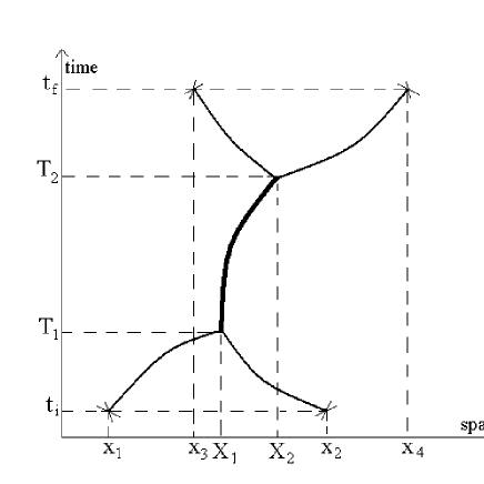
Figure 1: A typical tree path for D0-branes

Translating all the above to the momentum space is obtained by ($E_{k}=\frac{p_{k}^{2}}{2m_{0}}$ with $k=1,2,3,4$)

$$\langle p_{3},p_{4};t_{f}|p_{1},p_{2};t_{i}\rangle\sim{\rm e}^{i(E_{3}+E_{4})t_{f}-i(E_{1}+E_{2})t_{i}} \int\prod_{a=1}^{4}dx_{a}{\rm e}^{i(p_{1}x_{1}+p_{2}x_{2}-p_{3}x_{3}-p_{4}x_{4})}$$ (10)

$$\times\langle x_{3},x_{4};t_{f}|x_{1},x_{2};t_{i}\rangle.$$

This representation is useful to calculate the cross section. The integrals can be done easily to find

$$\langle p_{3},p_{4};t_{f}|p_{1},p_{2};t_{i}\rangle\sim\delta^{d}(p_{1}+p_{2}-p_{3}-p_{4})\int_{t_{i}}^{t_{f}}dT_{1}dT_{2}\theta(T_{2}-T_{1})$$ (11)

$$\times\exp(\frac{-i(p_{1}^{2}+p_{2}^{2})T_{1}}{2m_{0}})\exp(\frac{-iq^{2}(T_{2}-T_{1})}{4m_{0}})\exp(\frac{i(p_{3}^{2}+p_{4}^{2})T_{2}}{2m_{0}})$$

$$K_{oscillator}(Y_{\perp}=0,T_{2};Y_{\perp}=0,T_{1})$$

where $\vec{q}=\vec{p}_{1}+\vec{p}_{2}=\vec{p}_{3}+\vec{p}_{4}$.

To have a real scattering process one assumes

$$t_{i}\rightarrow-\infty,\;\;\;t_{f}\rightarrow\infty.$$

We put $T\equiv T_{2}-T_{1}$ which has the range $0\leq T\leq\infty$. The integrals yield

$$\langle p_{3},p_{4};\infty|p_{1},p_{2};-\infty\rangle \sim \delta^{d}(p_{1}+p_{2}-p_{3}-p_{4})\delta(\frac{p_{1}^{2}}{2m_{0}}+\frac{p_{2}^{2}}{2m_{0}}-\frac{p_{3}^{2}}{2m_{0}}-\frac{p_{4}^{2}}{2m_{0}})$$ (12)

$$\int_{0}^{\infty}dT\;{\rm e}^{\frac{-iT}{4m_{0}}(q^{2}-2(p_{1}^{2}+p_{2}^{2}))}\bigg{(}\frac{m_{0}\omega}{\sin(\omega T)}\bigg{)}^{d-1},$$

By recalling the the energy-momentum relation in Light-Cone gauge [14] one has:

$$2(p_{1}^{2}+p_{2}^{2})-q^{2}=2(2m_{0})(\frac{p_{1}^{2}+p_{2}^{2}}{2m_{0}})-q^{2}=2q_{+}q_{-}-q^{2}=q_{\mu}q^{\mu}\equiv q_{\mu}^{2}.$$

So it is found:

$$\langle p_{3},p_{4},E_{3},E_{4};\infty|p_{1},p_{2},E_{1},E_{2};-\infty\rangle \sim \delta^{d}(p_{1}+p_{2}-p_{3}-p_{4})\delta(E_{1}+E_{2}-E_{3}-E_{4})$$ (13)

$$\int_{0}^{\infty}dT{\rm e}^{\frac{-q_{\mu}^{2}}{4m_{0}}T}\bigg{(}\frac{m_{0}\omega}{\sin(\omega T)}\bigg{)}^{d-1}.$$

We perform a cut-off for $T$ in small values as $0<\epsilon\leq T\leq\infty$, with $\epsilon$ be small. By changing the integral variables as ${\rm e}^{-2\omega T}=\eta$ we have

$$\langle p_{3}^{\mu},p_{4}^{\mu};\infty|p_{1}^{\mu},p_{2},^{\mu};-\infty\rangle \sim \delta^{d}(p_{1}+p_{2}-p_{3}-p_{4})\delta(p_{-1}+p_{-2}-p_{-3}-p_{-4})$$ (14)

$$\frac{(m_{0}\omega)^{d-1}}{2\omega}\int_{0}^{x}d\eta\;\eta^{\frac{-q_{\mu}^{2}}{8m_{0}\omega}+\frac{d-3}{2}}(1-\eta)^{-d+1},$$

$$\sim \delta^{d}(p_{1}+p_{2}-p_{3}-p_{4})\delta(p_{-1}+p_{-2}-p_{-3}-p_{-4})$$

$$\frac{(m_{0}\omega)^{d-1}}{2\omega}B_{x}(\frac{-q_{\mu}^{2}}{8m_{0}\omega}+\frac{d-1}{2},-d+2)$$

with $1\sim x={\rm e}^{-2\omega\epsilon}$ and $B_{x}$ is the Incomplete Beta function. The longitudinal momentum conservation trivially is satisfied. Besides because of conservation of this momentum one can not expect so-called $t$-channel processes.

Polology

Equivalently one may use the other representation of $K_{oscillator}$ as

$$K_{oscillator}(Y_{\perp}=0,T_{2};Y_{\perp}=0,T_{1})=\sum_{n}\langle 0|n\rangle\langle n|0\rangle{\rm e}^{-iE_{n}(T_{2}-T_{1})},$$ (15)

with $E_{n}$’s as the known $H_{oscillator}$ eigenvalues. By this representation one finds the pole expansion [14]:

$$\langle p_{3},p_{4};\infty|p_{1},p_{2};-\infty\rangle \sim \delta^{d}(p_{1}+p_{2}-p_{3}-p_{4})\delta(p_{1+}+p_{2+}-p_{3+}-p_{4+})$$ (16)

$$\times\lim_{\epsilon\rightarrow 0^{+}}\sum_{n}C_{n}\;\frac{i4m_{0}}{q_{\mu}q^{\mu}-M_{n}^{2}+i\epsilon}.$$

This pole expansion also can be derived by extracting the poles of the amplitude (14) with the condition

$$\frac{-q_{\mu}^{2}}{8m_{0}\omega}+\frac{d-1}{2}=-n,\;\;{\rm with}\;n\;{\rm as\;a\;positive\;integer},$$ (17)

or

$$M_{n}^{2}=\frac{8k(n+\frac{d-1}{2})}{g_{s}^{2/3}l_{s}^{2}}.$$ (18)

4 Conclusion and Discussion

In this letter we calculate the cross section of two bosonic D0-branes to find a flavor about the cross section behavior of two hadrons with D0-branes as their partons. It is natural to take the results in elastic-large momentum transfer (Deep Elastic) regime. It was found that the cross section shows Regge behavior; the behavior with a long sounds in theoretical physics. This behavior has been used to insight to some aspects of hadron physics [15, 17, 18].

Why non-commutativity?
Special relativity in a modern compact definition may be represented as follows:
A modification of space-time to prepare it as a ground for the natural and theoretically consistent propagation of fields.

So one learns that the space-time makes a $X_{\mu}$ 4-vector which behaves like the electromagnetic gauge field $A_{\mu}$ (spin 1) under the boost transformations.

Also in this way supersymmetry (SUSY) is a natural continuation of the special relativity program:
Including spin $\frac{1}{2}$ sectors to the coordinates of space-time, as the fermions of nature. This leads one to the space-time formulation of the SUSY theories. Also it is the same way which one introduces fermions to the bosonic string theory.

Now, what may be modified if nature has non-abelian (non-commutative) gauge fields? In present nature non-abelian gauge fields can not make spatially long coherent states; they are confined or too heavy. But the picture may be changed inside a hadron or very near of an electron. In fact recent developments of string theories sound this change and it is understood that non-commutative coordinates and non-abelian gauge fields are two sides of one coin. The future theoretical research in this area may make clear the relations.

Acknowledgement

I am grateful to S. Parvizi for useful discussions.

References

- [1] J. Polchinski, ”Strings and QCD”, hep-th/9210045.
- [2] A.M. Polyakov, ”Gauge Fields and Strings”, Harwood Academic Publishers, Chur (1987).
- [3] A.M. Polyakov, Nucl. Phys. B486 (1997) 23; F. Quevedo and C.A. Trugenberger, Nucl. Phys. B501 (1997) 143; M.C. Diamantini and C.A. Trugenberger, ”Geometric Aspects of Confining Strings”, hep-th/9803046.
- [4] R. Peschanski, ”Is QCD at Small x a String Theory?”, hep-ph/9710483; ”Dual Shapiro-Virasoro Amplitudes in The QCD Dipole Picture”, Phys. Lett. B409 (1997) 491, hep-ph/9704342; A. Bialas, H. Navelet and R. Peschanski, ”The QCD Triple Pomeron Coupling from String Amplitudes”, hep-ph/9711442.
- [5] S.S. Gubser, I.R. Klebanov and A.M. Polyakov, ”Gauge Theory Correlators from Non-Critical String Theory”, hep-th/9802109.
- [6] M.V. Polyakov and V.V. Vereshagin, ”Effective Chiral Lagrangian from Dual Resonance Models”, Phys. Rev. D54 (1996) 1112, hep-ph/9509259; M.V. Polyakov and G. Weidl, ”Chiral Expansions in the Dual(String) Models of Goldstone Meson Scattering”, hep-ph/9612486.
- [7] J.H. Schwartz, ”Lectures on Superstring and M-Theory Dualities”, hep-th/9607201; C. Vafa, ”Lectures on String and Dualities”, hep-th/9702201; A. Sen, ”An Introduction to Nonperturbative String Theory”, hep-th/9802051; E. Kiritsis, ”An Introduction to Nonperturbative String Theory”, hep-th/9708130.
- [8] J. Polchinski, Phys. Rev. Lett. 75 (1995) 4724, hep-th/9510017.
- [9] J. Polchinski, ”Tasi Lectures on D-Branes”, hep-th/9611050.
- [10] F.E. Close, ”An Introduction to Quarks and Partons ”, Academic Press (1979).
- [11] S. Beane, Phys. Rev. D59 (1998) 036001.
- [12] A.H. Fatollahi, ”Do Quarks Obey D-Brane Dynamics?”, hep-ph/9902414.
- [13] W. Lucha, F. Schoberl and D. Gromes, Phys. Rep. 200 (1991) 127; S. Mukherjee, et. al., Phys. Rep. 231 (1993) 201.
- [14] S. Parvizi and A.H. Fatollahi, ”D-Particle Feynman Graphs and Their Amplitudes”, hep-th/9907146.
- [15] A. Donnachie and P.V. Landshoff, Phys. Lett. B296 (1992) 227.
- [16] A. Levy, ”Low- Physics at HERA”, DESY-97-013, TAUP-2398-96.
- [17] J.R. Cudell, A. Donnachie and P.V. Landshoff, ”Perturbative Evolution and Regge Theory”, hep-ph/9901222.
- [18] A. Donnachie and P.V. Landshoff, ”Small x: Two Pomerons” Phys. Lett. B437 (1998) 408, hep-ph/9806344.
- [19] E. Witten, Nucl. Phys. B460 (1996) 335, hep-th/9510135.
- [20] W. Taylor, ”Lectures on D-Branes, Gauge Theory and M(atrices)”, hep-th/9801182; C. Gomes and R. Hernandez, ”Fields, Strings and Branes”, hep-th/9711102; R. Dijkgraaf, ”Les Houches Lectures on Fields, Strings and Duality” , hep-th/9703136.
- [21] T. Banks, ”Matrix Theory”, hep-th/9710231.
- [22] D. Kabat and P. Pouliot, Phys. Rev. Lett. 77 (1996) 1004, hep-th/9603127; U.H. Danielsson, G. Ferretti and B. Sundborg, Int. J. Mod. Phys. A11 (1996) 5463, hep-th/9603081.