Flux tube dynamics in the dual superconductor

Abstract

We study plasma oscillations in a flux tube of the dual superconductor model of ’t Hooft and Mandelstam. A magnetic condensate is coupled to an electromagnetic field by its dual vector potential, and fixed electric charges set up a flux tube. An electrically charged fluid (a quark plasma) flows in the tube and screens the fixed charges via plasma oscillations. We investigate both Type I and Type II superconductors, with plasma frequencies both above and below the threshold for radiation into the Higgs vacuum. We find strong radiation of electric flux into the superconductor in all regimes, and argue that this invalidates the use of the simplest dual superconductor model for dynamical problems.

I Introduction

The confinement of color in quantum chromodynamics is explained if color electric fields form flux tubes. These flux tubes appear readily in the bag model [1], but this is a geometric picture rather than a dynamical one. ’t Hooft [2] and Mandelstam [3] proposed that, just as magnetic flux tubes form in a superconductor [4], a condensation of magnetic charge in the QCD vacuum would lead to the formation of electric flux tubes and confinement. This is the dual superconductor picture of confinement.

The analytical study of the confining flux tube depends largely on a classical, Abelian model. One can connect this model to QCD with ’t Hooft’s idea of Abelian dominance [5]. Starting in QCD, one fixes an Abelian gauge and asserts that the dominant degrees of freedom are Abelian gauge fields (from a Cartan subalgebra) and Abelian magnetic monopoles, with weak coupling to the non-Abelian gauge fields which assume the guise of self-coupled charged fields. The assumption that the effective interaction of the monopoles causes their condensation leads immediately to the dual superconductor picture. The validity of this scenario is a subject of research and debate in the lattice gauge theory community [6].

In superconductivity, one studies the static structure of magnetic flux tubes via a Landau-Ginzburg theory [7]. The simplest Landau-Ginzburg Hamiltonian is that of the Abelian Higgs model in three dimensions. Classical solutions of the Abelian Higgs theory have been considered as models of QCD’s electric flux tube as well [8, 9, 10, 11, 12]. Suganuma, Sasaki, and Toki and their collaborators [13, 14], using the formalism proposed by Suzuki [15], have fixed the effective coupling constants of the Abelian Higgs model by comparing its flux tube with phenomenology. There have also been attempts to do so by comparison with the flux tube that emerges in lattice gauge theory [16]. Success in this program will establish a Landau-Ginzburg effective Hamiltonian of QCD.

In this paper we present a study not of the statics of the confining flux tube, but of its dynamics. The flux tube of QCD is not a static object. Creation of flux tubes and their subsequent decay through pair creation offer a detailed model of particle creation in $e^{+}e^{-}$, $pp$, and $pA$ collisions [17, 18]. In the case of nucleus–nucleus collisions, the flux tube has an appreciable transverse extent, so that it can be called a “color capacitor” if the color field is coherent across it, or a “color rope” [19] if it is not. $q\bar{q}$ pairs and gluons are created through the Schwinger pair creation process [20], and they screen the field in the flux tube while carrying away the energy in the form of hadrons. If the density of created particles is large enough, the quarks and gluons form a quark–gluon plasma before the final hadronization takes place.

Field-theoretic analysis of pair creation and back-reaction in the flux tube [21] has shown the buildup of particle density and subsequent plasma oscillations. The methods were applied first to a field region of infinite spatial extent, rather than to a finite flux tube. Eisenberg [22] carried out a calculation in a cylindrical flux tube of fixed radius, as suggested by the bag model. In our study here, the flux tube is a dynamical field configuration, not a static geometric object.

Following [15] and [13], we set up the electric flux tube in classical electrodynamics coupled to an Abelian Higgs field via the dual gauge field. Thus the Higgs field represents a condensate of magnetic monopoles; the dual Meissner effect confines electric flux to flux tubes. Starting from a static flux tube configuration, we release a density of electric charges in the system and allow them to accelerate and screen the electric field. The weakening of the electric field allows the flux tube to collapse, but the inertia of the charges carries them into plasma oscillations that build up the field strength again and force open the tube. The coupling of the plasma oscillations to the Higgs field making up the flux tube is the main new feature in our work.

In Section II we describe the dual superconductor theory. The model contains an Abelian gauge field governed by Maxwell’s equations, with coupling to electric charges and currents on the one hand and to a magnetic Higgs field on the other. The electric currents are treated hydrodynamically; the Higgs field is a classical field that confines electric flux to the tube. The coupling to the Higgs field is accomplished by means of a dual vector potential, as introduced by Zwanziger [23] and used subsequently in [8] for the static problem and in [13, 14] for phenomenological modeling. We impose cylindrical symmetry and we assume $z$-independence along the flux tube in the region far from its ends. Nevertheless, we are forced to pay some attention to what happens near the ends of the tube in order to define potentials unambiguously.

We present numerical results in Section III. We set the parameters of the theory in both the Type I and Type II regimes, and show how plasma oscillations arise. We consider plasma frequencies both above and below the cutoff for radiation into the Higgs vacuum. The plasma oscillations are accompanied by changes in the radius of the flux tube as the electric pressure from within decreases through screening, only to increase again as the currents overshoot.

We believe that this paper is the first to address the dynamics of an electric flux tube within this model. It is amusing to note that this physical situation has no counterpart in superconductivity. While our magnetic Higgs field appears in the usual Landau-Ginzburg theory as an electrically charged condensate, our electric currents cannot appear there because there are no magnetic monopoles in nature. An Abrikosov flux tube has to run all the way to the boundary of the sample, where it joins onto the external magnetic field. Our electric flux tube, on the other hand, has a finite (but large) length, and the charges at its ends can be screened by the electric currents that flow in it. We review in the appendix the well-known phenomenon of flux quantization and why it has no effect on a flux tube of finite length.

II Field equations in cylindrical geometry

Our classical model for the flux tube is electrodynamics coupled to a scalar magnetic monopole field. The equations of motion are Maxwell’s equations with both electric and magnetic sources, plus the Klein-Gordon equation for the monopoles. The latter is coupled not to the usual vector potential $A_{\mu}$ but to the dual potential [23] $B_{\mu}$, and contains a self-interaction that puts it into the Higgs phase.

We make a cylindrically symmetric ansatz for the fields, and furthermore assume $z$-independence far from the sources at the ends of the tube. We put the electrically charged sources on the $z$ axis at $z=\pm z_{0}$, and we assume that all the space-charge effects are localized there. The central region is defined by $|z|<z_{1}$, where $z_{1}<z_{0}$ is chosen to exclude the end regions (see Fig. 1).

A Maxwell’s equations

Maxwell’s equations with electric and magnetic currents are

$$\partial_{\mu}F^{\mu\nu} = j_{e}^{\nu}$$ (1)

$$\partial_{\mu}\tilde{F}^{\mu\nu} = j_{g}^{\nu}\>,$$ (2)

where $\tilde{F}^{\mu\nu}=\frac{1}{2}\epsilon^{\mu\nu\lambda\sigma}F_{\lambda\sigma}$. Eq. (2) replaces the Bianchi identity of ordinary electrodynamics. We can solve it with a vector potential, but there is a new term,

$$F^{\mu\nu}=\partial^{\mu}A^{\nu}-\partial^{\nu}A^{\mu}+\epsilon^{\mu\nu\lambda\sigma}G_{\lambda\sigma}\>.$$ (3)

Defining an arbitrary vector $n^{\mu}$, one finds that (2) is solved if

$$G^{\mu\nu}=-n^{\mu}(n\cdot\partial)^{-1}j_{g}^{\nu}\>,$$ (4)

where $(n\cdot\partial)^{-1}$ represents an integration from infinity with suitable boundary conditions. The field equation for $A_{\mu}$ then follows from (1). Solving Maxwell’s equations in the opposite order, the same field strength can be represented alternatively by a dual vector potential, according to

$$\tilde{F}^{\mu\nu}=\partial^{\mu}B^{\nu}-\partial^{\nu}B^{\mu}+\epsilon^{\mu\nu\lambda\sigma}M_{\lambda\sigma}\>,$$ (5)

with

$$M^{\mu\nu}=-n^{\mu}(n\cdot\partial)^{-1}j_{e}^{\nu}\>,$$ (6)

in order to satisfy (1). Now the field equation for $B_{\mu}$ follows from (2). We will return to the vector potentials below.

In three-dimensional notation,

$$\nabla\cdot{\bf E}=\rho_{e}$$ (8)

$$\nabla\times{\bf H}-\frac{\partial{\bf E}}{\partial t}={\bf j}_{e}$$ (9)

$$\nabla\cdot{\bf H}=\rho_{g}$$ (10)

$$\nabla\times{\bf E}+\frac{\partial{\bf H}}{\partial t}=-{\bf j}_{g}$$ (11)

In the aforementioned central region $|z|<z_{1}$, we make the ansatz

$${\bf E}=E(r,t)\,\hat{\bf z}$$ (13)

$${\bf H}=H(r,t)\,\hat{\boldmath\theta}$$ (14)

$${\bf j}_{e}=j_{e}(r,t)\,\hat{\bf z}$$ (15)

$${\bf j}_{g}=j_{g}(r,t)\,\hat{\boldmath\theta}$$ (16)

Ampère’s Law (9) has only a $\hat{\bf z}$ component,

$$\frac{1}{r}\frac{\partial}{\partial r}\left(rH\right)-\frac{\partial E}{\partial t}=j_{e}\>,$$ (17)

and Faraday’s Law (11) has only a $\hat{\boldmath\theta}$ component,

$$-\frac{\partial E}{\partial r}+\frac{\partial H}{\partial t}=-j_{g}\>.$$ (18)

The two Gauss laws show that the charge densities are zero,

$$\rho_{e}=\rho_{g}=0\>.$$ (19)

Eqs. (17) and (18) are the equations of motion for $E$ and $H$.

Near the ends of the flux tube, $|z|>z_{1}$, we must allow for new components $E_{r}$ and $j_{er}$, as well as for $\rho_{e}$, and all fields will be $z$-dependent.

B Vector potentials

In order to calculate the time evolution of the matter fields, we need the vector potentials. In fact, we need only the dual potential $B_{\mu}$ [26], which enters the field equation for the monopole field. From (5) and (6),

$${\bf E} = -\nabla\times{\bf B}+\hat{\bf z}(\hat{\bf z}\cdot\nabla)^{-1}\rho_{e}$$ (20)

$${\bf H} = -\nabla B^{0}-\frac{\partial{\bf B}}{\partial t}-(\hat{\bf z}\cdot\nabla)^{-1}(\hat{\bf z}\times{\bf j}_{e})\>,$$ (21)

where we have chosen $n^{\mu}=(0,\hat{\bf z})$. We choose the gauge $B_{0}=0$. Inverting (20) gives

$${\bf B}=(\hat{\bf z}\cdot\nabla)^{-1}(\hat{\bf z}\times{\bf E})\>.$$ (22)

Our ansatz for ${\bf E}$ then gives ${\bf B}=B\,\hat{\boldmath\theta}$, with

$$B(r,z)=\int_{-\infty}^{z}E_{r}(r,z^{\prime})\,dz^{\prime}\>.$$ (23)

This integral only gets contributions from the regions around the sources, since $E_{r}=0$ far from the charges. This makes $B$ independent of $z$ in the central region $|z|<z_{1}$. We can relate the integral in (23) to the charge distribution near the sources as follows. We take a cylindrical surface of radius $r$ with ends at $-\infty$ and $-z_{1}$. Gauss’ Law gives for this surface

$$Q(r)=2\pi r\int_{-\infty}^{-z_{1}}E_{r}(r,z)\,dz+2\pi\int_{0}^{r}E_{z}(r^{\prime},-z_{1})\,r^{\prime}\,dr^{\prime}\>,$$ (24)

where $Q(r)$ is the charge inside the cylinder (composed of the original source plus the space charge around it). Noting that $E_{z}(r^{\prime},-z_{1})$ is the $z$-independent $E_{z}(r^{\prime})$, we obtain the relation

$$B(r)=\frac{Q(r)}{2\pi r}-\frac{1}{r}\int_{0}^{r}E_{z}(r^{\prime})\,r^{\prime}\,dr^{\prime}$$ (25)

and its inverse

$$E\equiv E_{z}=-\frac{1}{r}\frac{\partial}{\partial r}(rB)+\frac{1}{2\pi r}\frac{\partial Q}{\partial r}\>.$$ (26)

Given $E$ and some model for the charge $Q(r)$ (see below), we can calculate $B$.

C Magnetic monopoles

The magnetic monopoles are represented by a classical Klein-Gordon equation with a Higgs potential,

$$D_{\mu}^{B}D^{\mu B}\psi+\lambda(|\psi|^{2}-v^{2})\psi=0\>,$$ (27)

where

$$D^{B}_{\mu}\equiv\partial_{\mu}-igB_{\mu}\>.$$ (28)

We make the ansatz $\psi=\rho(r,t)e^{i\chi_{g}(\theta)}$, giving

$$\left[\frac{\partial^{2}}{\partial t^{2}}-\frac{1}{r}\frac{\partial}{\partial r}r\frac{\partial}{\partial r}-\left(\frac{1}{r}\frac{\partial}{\partial\theta}-igB\right)^{2}\right]\rho e^{i\chi}+\lambda\left(\rho^{2}-v^{2}\right)\rho e^{i\chi}=0\>.$$ (29)

We assume $\chi_{g}=n\theta$ (for a flux tube with $n$ units of electric flux), so

$$\left[\frac{\partial^{2}}{\partial t^{2}}-\frac{1}{r}\frac{\partial}{\partial r}r\frac{\partial}{\partial r}+\left(\frac{n}{r}-gB\right)^{2}\right]\rho+\lambda\left(\rho^{2}-v^{2}\right)\rho=0\>.$$ (30)

This is the equation of motion for $\rho$. It feeds back into Maxwell’s equations via the magnetic current,

$${\bf j}_{g}=2g\rho^{2}\left(\nabla\chi_{g}-g{\bf B}\right)$$ (31)

which contains only a $\hat{\boldmath\theta}$ component,

$$j_{g}=2g\rho^{2}\left(\frac{n}{r}-gB\right)\ .$$ (32)

As shown in the Appendix, $n$ represents electric flux coming in from infinity, so that we will set $n=0$ for simplicity. The flux generated by $Q$ at the ends of the flux tube is not quantized.

D Charged matter

We represent the electrically charged matter by classical two-fluid magnetohydrodynamics. The positively and negatively charged fluids both have particle density $n_{e}(r,t)$ (so that $\rho_{e}=0$) and their velocities are ${\bf v}^{\pm}$. The fluid motion is determined by Euler’s equations

$$m\left[\frac{\partial{\bf v}^{\pm}}{\partial t}+({\bf v}^{\pm}\cdot\nabla){\bf v}^{\pm}\right]=\pm e{\bf E}\pm e{\bf v}^{\pm}\times{\bf H}-\frac{1}{n_{e}}{\nabla P}$$ (33)

and the continuity equation

$$\frac{\partial n_{e}}{\partial t}+\nabla\cdot(n_{e}{\bf v}^{\pm})=0\>.$$ (34)

The electric current is given by

$${\bf j}_{e}=n_{e}e\left({\bf v}^{+}-{\bf v}^{-}\right)\>.$$ (35)

We assume in the central region that all quantities depend only on $r$ and $t$, so that ${\bf v}^{\pm}\cdot\nabla=v^{\pm}_{r}\frac{\partial}{\partial r}$. Recalling that ${\bf E}=E\,\hat{\bf z}$ and ${\bf H}=H\,\hat{\boldmath\theta}$, we have

$$m\frac{\partial}{\partial t}v^{\pm}_{r} = -mv^{\pm}_{r}\frac{\partial}{\partial r}v^{\pm}_{r}\mp ev^{\pm}_{z}H-\frac{1}{n_{e}}\frac{\partial P}{\partial r}$$ (36)

$$m\frac{\partial}{\partial t}v^{\pm}_{z} = -mv^{\pm}_{r}\frac{\partial}{\partial r}v^{\pm}_{z}\pm eE\pm ev^{\pm}_{r}H$$ (37)

and

$$\frac{\partial n_{e}}{\partial t}=-v^{\pm}_{r}\frac{\partial n_{e}}{\partial r}-\frac{n_{e}}{r}\frac{\partial}{\partial r}(rv^{\pm}_{r})\>.$$ (38)

Not surprisingly, these equations allow the ansatz

$$v_{r}^{+} = v_{r}^{-}\equiv v_{r}$$

$$v_{z}^{+} = -v_{z}^{-}\equiv v_{z}\>,$$

we find

$$m\frac{\partial}{\partial t}v_{r} = -mv_{r}\frac{\partial}{\partial r}v_{r}-ev_{z}H-\frac{1}{n_{e}}\frac{\partial P}{\partial r}$$ (39)

$$m\frac{\partial}{\partial t}v_{z} = -mv_{r}\frac{\partial}{\partial r}v_{z}+eE+ev_{r}H$$ (40)

$$\frac{\partial n_{e}}{\partial t} = -v_{r}\frac{\partial n_{e}}{\partial r}-\frac{n_{e}}{r}\frac{\partial}{\partial r}(rv_{r})\>.$$ (41)

These equations feed back into Maxwell’s equations via the current, which is in the $\hat{\bf z}$ direction and has the magnitude

$$j_{e}=2n_{e}ev_{z}\>.$$ (42)

We need an equation of state to relate $P$ to $n_{e}$. Having in mind a quark–gluon plasma, we choose the equation of state of a relativistic ideal gas with the appropriate number of massless fermions and bosons. We set the chemical potential to zero and write all quantities in terms of the temperature,

$$P = 37\frac{\pi^{2}}{90}T^{4}$$ (43)

$$n_{e} = 37\frac{\zeta(3)}{\pi^{2}}T^{3}\>.$$ (44)

Then eqs. (41) can be written in terms of the velocities and temperature as

$$m\frac{\partial}{\partial t}v_{r} = -mv_{r}\frac{\partial}{\partial r}v_{r}-ev_{z}H-\frac{4\pi^{4}}{90\zeta(3)}\frac{\partial T}{\partial r}$$ (45)

$$m\frac{\partial}{\partial t}v_{z} = -mv_{r}\frac{\partial}{\partial r}v_{z}+eE+ev_{r}H$$ (46)

$$\frac{\partial T}{\partial t} = -v_{r}\frac{\partial T}{\partial r}-\frac{T}{3r}\frac{\partial}{\partial r}(rv_{r})\>.$$ (47)

The advantage of a hydrodynamic description of the charged matter is that the fluid interacts directly with the field strengths E and H. If we were to consider classical or quantum field theory instead of hydrodynamics, we would need the vector potential ${\bf A}$. In our geometry, the simplest ansatz would require two components, $A_{r}$ and $A_{z}$. The potential would necessarily be $z$-dependent in the central region; moreover, the simplified treatment of the ends of the flux tube (see below) would be impossible.

E The ends of the flux tube

For study of the central region, all we need to know about the complex regions at the ends of the flux tube is $Q(r)$, which represents the charge density built up near $-z_{0}$ by the current ${\bf j}_{e}$. (The region near $z=+z_{0}$ is, of course, a mirror image of the region near $-z_{0}$.) Without dealing in detail with the motion of charges near the ends of the flux tube, we can guess at a few models:

1. Point charge: Here we just assume that all the current merely accumulates in a point charge at $z=-z_{0}$. Then $Q(r,t)$ is independent of $r$, and charge conservation gives

   $$\frac{dQ}{dt}=-2\pi\int_{0}^{\infty}j_{e}(r)\,r\,dr\>.$$ (48)

2. Surface charge density: Here we let the charge pile up on a plate near $z=-z_{0}$, giving a surface charge density $\sigma(r,t)$. Then

   $$Q(r,t)=2\pi\int_{0}^{r}\sigma(r^{\prime},t)\,r^{\prime}\,dr^{\prime}$$ (49)

   and

   $$\frac{\partial\sigma}{\partial t}=-j_{e}\>.$$ (50)

   Initial conditions have to be specified for $\sigma$ to represent the original source of the flux tube.

3. Both: Keeping the initial charge pointlike, we put only the accumulated charge into $\sigma$. Then

   $$Q(r,t)=Q_{0}+2\pi\int_{0}^{r}\sigma(r^{\prime},t)\,r^{\prime}\,dr^{\prime}$$ (51)

   and $\sigma$ is determined by (50) as above. The initial condition is $\sigma=0$. Note that in this case the space charge will never exactly cancel $Q_{0}$ and thus any plasma oscillations will be asymmetric.

The initial conditions must in any case satisfy Gauss’ Law,

$$2\pi\int_{0}^{\infty}E(r)r\,dr=Q(\infty)\>,$$ (52)

if there is no flux coming from infinity (i.e., $n=0$).

F Initial conditions

We start off the system in the configuration of a static flux tube with a stationary fluid in it. We combine the static limit of (18) with (26) and (32) to give

$$\frac{\partial}{\partial r}\frac{1}{r}\frac{\partial}{\partial r}\left[rB(r)-\frac{1}{2\pi}Q(r)\right]=2g^{2}\rho^{2}B\>,$$ (53)

where we have chosen $n=0$. Eq. (25) gives the boundary condition $B(0)=0$ unless $Q$ includes a point charge $Q_{0}$; in that case

$$B(r)\sim\frac{Q_{0}}{2\pi r}$$ (54)

as $r\to 0$. Eq. (25) together with (52) gives $rB(r)\to 0$ at infinity.

The static limit of the Klein-Gordon equation (30) is

$$\left[-\frac{1}{r}\frac{\partial}{\partial r}r\frac{\partial}{\partial r}+g^{2}B^{2}\right]\rho+\lambda\left(\rho^{2}-v^{2}\right)\rho=0\>,$$ (55)

with the boundary conditions that $\rho$ is zero at the origin and tends to $\rho=v$ at infinity.

Focusing on the case where $Q$ is a point charge, we define the reduced field $b(r)$ via

$$B=\frac{Q}{2\pi r}b\>,$$ (56)

giving

$$b^{\prime\prime}-\frac{b^{\prime}}{r}-2g^{2}\rho^{2}b=0\>,$$ (57)

with $b(0)=1$ and $b(\infty)=0$, and

$$-\rho^{\prime\prime}-\frac{\rho^{\prime}}{r}+\left[\left(\frac{Qg}{2\pi}\frac{b}{r}\right)^{2}+\lambda(\rho^{2}-v^{2})\right]\rho=0\>.$$ (58)

These equations determine $\rho$ and $B$, and hence $E$, for the static flux tube. Clearly $H=0$ here.

III Plasma oscillations

We determine the time evolution of the system through the following system of equations. The Maxwell equations (17) and (18) give E and H; the MHD equations (47) give v and $T$, and hence ${\bf j}_{e}$ via (42) and (44). Eq. (48) gives the charge $Q$ whence (25) gives the vector potential B. The scalar field $\rho$ evolves according to the Klein-Gordon equation (30), and (32) gives the magnetic current ${\bf j}_{g}$, the last ingredient for the Maxwell equations. The initial conditions, as noted, consist of the static flux tube with an initial value of $Q$, and of a static fluid distribution specified by $T(r)$.

We choose four sets of parameters, listed in Table I. The magnetic charge $g$ and the vacuum expectation value $v=\rho(r\to\infty)$ determine the vector mass $m_{V}=\sqrt{2}gv$ and its reciprocal, the London penetration depth $\lambda_{L}=m_{V}^{-1}$. The scalar self-coupling $\lambda$ determines, along with $v$, the (dual) Higgs mass $m_{H}=\sqrt{2\lambda}v$ and the Ginzburg-Landau coherence length $\xi=m_{H}^{-1}$. The ratio of these lengths is $\kappa=\lambda_{L}/\xi=\sqrt{\lambda}/g$. If this value is smaller than one then the superconductor is of Type I; otherwise it is of Type II.

In ordinary superconductors, flux tubes are observed only in Type II materials, when the applied magnetic field lies between the critical values $H_{c1}$ and $H_{c2}$ and penetrates via creation of an Abrikosov lattice. Type I materials, on the other hand, expel the field entirely as long as superconductivity persists. The situation would be different if one were to introduce a pair of magnetic monopoles. Then the magnetic field would be forced into a flux tube between the monopoles, even in a Type I material. The difference between Type I and II would lie in the stability of the flux tube against splitting into a lattice (a “rope”) of smaller tubes: Type I tubes would be stable, while Type II tubes would split. This splitting is presumably inaccessible from our cylindrically symmetric ansatz.

The values of $\lambda$ and $g$ fixed phenomenologically in [13] are in the Type II region, and we choose these values for our Type II cases. For Type I, we increase $g$ and decrease $\lambda$ to make $\kappa<1$. We take $v=126$ MeV from [13] as well. We fix the electric charge $e$ according to the Dirac quantization condition $eg/4\pi=1$, even though this is not meaningful for continuum hydrodynamics.

The charged fluid presents a conundrum. Our intuition about confinement suggests that the superconducting vacuum should expel this matter, and thus confine it to the flux tube. (This happens in the Friedberg–Lee Model [25].) In this Abelian theory, however, the locally neutral fluid is not confined. If the initial conditions contain a fluid inside the flux tube only, it will flow outward in a hydrodynamic rarefaction wave. Perhaps the fluid outside the flux tube may be interpreted as a hadronic fluid. In any case, we prefer not to superimpose radial hydrodynamic flow on the oscillations of the flux tube. Thus we choose a uniform initial fluid density, outside the flux tube as well as inside. Having in mind a quark–gluon plasma, we set the initial temperature to be spatially uniform with $T_{0}$ = 150 MeV.

The initial value $Q_{0}$ of the charge at the ends of the flux tube gives the initial amount of electric flux. In a $pp$ collision, one would have $Q_{0}\sim e$, corresponding to the creation of a flux tube in the fundamental representation; an $AA$ collision between heavy nuclei would give[19, 27] $Q_{0}\sim A^{1/3}e$, which reaches $Q_{0}\sim 6e$ for large nuclei. A large value of $Q_{0}$ will give a thick flux tube and large-amplitude plasma oscillations, and thus enhance the non-linear effects due to the Higgs coupling. Unfortunately, very large values of $Q_{0}$ are outside the range of stability of our numerics; we choose values that are as large as possible given this constraint.

The plasma frequency is

$$\omega_{p}=\sqrt{\frac{2n_{e}e^{2}}{m}}\>,$$ (59)

where the factor of two reflects the fact that we have two fluids. For given $n_{e}$ and $e$, we fix $m$ so as to tune $\omega_{p}$ to either side of the vector mass $m_{V}$; thus the plasma oscillations will occur at frequencies either above or below the threshold for radiation. We expect a priori that $m$ will be in the neighborhood of the dynamical mass $eT$ of light particles in a heat bath. The parameters used in [13] give a rather small vector mass, and with $e$ = $4\pi/g$ the condition $\omega_{p}<m_{V}$ leads to an unreasonably large value of $m$. Instead we choose in this case to lower the value of the electric charge to $e=1$.

Case 1.

Fig. 2 shows plasma oscillations in the on-axis electric field for the Type I superconductor with $\omega_{p}<m_{V}$. The oscillations are clearly nonlinear, with varying amplitude and misshapen waveform. Fig. 3 contains snapshots taken at the times of maxima in $E(r=0)$. These snapshots show radiation emanating from the flux tube in both $E$ and $\rho$. The plots of $rE$ show that the oscillating electric flux in the outgoing wave is as large in amplitude as the initial flux distribution. It is difficult to tell, however, whether the wave amplitude decays as $r^{-1/2}$, as expected for a true propagating wave, or as $r^{-1}$, which would make the wave evanescent.

Since the frequency of the plasma oscillations is below the vector mass, this cannot be simple linear radiation. The third row of fig. 3, indeed, shows strong coupling of the nonlinear $\rho$ field to the electromagnetic wave. The origin of this coupling, shown in fig. 4, is the collapse of the flux tube under the pressure of the $\rho$ field when the electric field is weak. The figure shows snapshots of $\rho$ taken in the first half-cycle of the evolution. The middle snapshot, taken when $E(r=0)=0$, shows appreciable narrowing of the flux tube core even as $\rho$ is driven downward at larger radii in the first oscillation of the outgoing wave.

Case 2.

Oscillations in the Type I superconductor with a larger plasma frequency, $\omega_{p}>m_{V}$, are shown in figs. 5 and 6. Here the irregularity of the waveform of $E(r=0)$ is due to ordinary radiation in interaction with a more-or-less static flux tube wall. Again there is appreciable electric flux radiated outward, but there is little effect on the $\rho$ field. This is because the latter cannot respond when driven by the high-frequency electromagnetic oscillations. We note that the larger value of $gQ_{0}$ here creates a thicker flux tube and keeps more flux in the flux tube despite the radiation.

Case 3.

The Type II superconductor with $\omega_{p}<m_{V}$ is similar in behavior to the Type I system. The smaller plasma frequency makes it difficult to calculate through more than two or three oscillations, in spite of the high stability of the Crank-Nicholson algorithm we use. In fig. 7 we see strong deformation of the waveform. Fig. 8 shows radiation similar to the Type I case, but the perturbation of the $\rho$ field is less apparent.

Case 4.

Finally, the corresponding plots for the Type II superconductor with $\omega_{p}>m_{V}$ show considerable structure. Recall that this parameter set is that used in [13] for phenomenological fits to static quantities. The oscillations shown in fig. 9 are too rapid to couple strongly to $\rho$, and we see strong electromagnetic radiation (figs. 10 and 11) accompanied by weak high-momentum disturbances in $\rho$.

IV Discussion

Our numerical results raise difficulties for the dual superconductor picture of confinement. As a static model, the dual superconductor does indeed form flux tubes that confine charges in string-like configurations. Once the dynamics are examined, however, the lack of absolute color confinement becomes apparent. While the motion of neutral particle matter outside the flux tube may be passed off as the emission of color-neutral hadrons, the radiation of appreciable electric flux cannot. The electric field in ’t Hooft’s Abelian projection is after all a color field, representing a coherent, colored gluon state.

It was predictable that oscillations with $\omega_{p}>m_{V}$ would radiate into the Higgs vacuum, since the photon does have a less-than-infinite mass. One might be tempted to restrict application of the dual superconductor model to situations where frequencies are much less than $m_{V}$. We have seen, however, that this is insufficient. Even low-frequency plasma oscillations, where radiation should be impossible, succeed in spreading out the electric flux via nonlinear effects. Thus the model is not reliable even in this regime. It is possible that the model can be made applicable to low-frequency physics by choosing a monopole Lagrangian more general than the $\psi^{4}$ of the simplest Landau-Ginzburg theory. Absolute confinement, however, will never be realized in this way. (The introduction of a strongly nonlinear dielectric constant is what enables the Friedberg–Lee model to confine all color fields, but this model has not been derived from QCD.)

’t Hooft’s Abelian reduction rests on the identification of the important degrees of freedom in an Abelian gauge. It is supposed that the magnetic monopoles have a strong self-interaction, leading to their condensation; that the Abelian gluons, belonging to the Cartan subalgebra, turn this condensate into a superconductor; and, most important, that the off-diagonal gluons are irrelevant to confinement, except insofar as they screen zero-triality states. These off-diagonal gluons, however, retain all the self-couplings of the original non-Abelian gauge theory. We conjecture that they are essential to understanding time-dependent phenomena related to confinement.

Flux quantization

Flux quantization, as it turns out, affects only flux coming in from infinity and not the flux due to the charge $Q$ at the ends of the flux tube. The quantization condition comes from demanding that the total energy be finite [28]. The energy of the monopole field contains the term

$$E_{\text{static}}\equiv\int d^{3}x\,\left|{\bf D}^{B}\psi\right|^{2}\>.$$ (60)

As $x^{2}+y^{2}\to\infty$, we have $\psi\to\psi_{0}e^{i\chi(\theta)}$ and ${\bf B}\to B\,\hat{\boldmath\theta}$, and thus the integrand approaches

$$\varepsilon_{\infty}\equiv\psi_{0}^{2}\cdot\left(\frac{\chi^{\prime}(\theta)}{r}-gB\right)^{2}\>.$$ (61)

In order that $\int^{\infty}r\,dr\,d\theta\,\varepsilon$ be finite, we must have at large $r$ that

$$\frac{d\chi}{d\theta}=gBr\>.$$ (62)

Since $\chi$ is only determined up to a multiple of $2\pi$, it can gain such a multiple when one goes around the circle. Integrating (62) over the circle at fixed $r$ gives

$$2\pi n=g\int Br\,d\theta=g\oint{\bf B}\cdot d{\bf l}\>,$$ (63)

where $n$ is an integer. In view of (20),

$$\oint{\bf B}\cdot d{\bf l}=\int(\nabla\times{\bf B})\cdot d{\bf S}=-\int{\bf E}\cdot d{\bf S}+Q=-\Phi_{E}+Q$$ (64)

where $\Phi_{E}$ is the total electric flux. Thus

$$\Phi_{E}=Q-2\pi n/g\>.$$ (65)

Only the external flux, the flux that does not end at $Q$, is quantized in units of $2\pi/g$. Choosing $\Phi_{E}=Q$, i.e., no external flux, means setting $n=0$.

TABLE I.: Parameters used in numerical simulations. $v=126$ MeV in all cases, and the initial temperature is $T_{0}=150$ MeV.

	$TypeI$	$TypeI$	$TypeII$	$TypeII$
	$\omega_{p}<m_{V}$	$\omega_{p}>m_{V}$	$\omega_{p}<m_{V}$	$\omega_{p}>m_{V}$
$\lambda$	$10.$	$10.$	$25.$	$25.$
$g$	$5.5$	$5.5$	$2.3$	$2.3$
$e$	$2.3$	$2.3$	$1.0$	$5.5$
$m_{V}$ (MeV)	$975.$	$975.$	$411.$	$411.$
$m_{H}$ (MeV)	$565.$	$565.$	$893.$	$893.$
$\lambda_{L}$ (fm)	$0.20$	$0.20$	$0.48$	$0.48$
$\xi$ (fm)	$0.35$	$0.35$	$0.22$	$0.22$
$\kappa$	$0.58$	$0.58$	$2.18$	$2.18$
$m$ (MeV)	$250.$	$50.$	$250.$	$50.$
$\omega_{p}$ (MeV)	$790.$	$1766.$	$343.$	$4192.$
$T_{p}=2\pi/\omega_{p}$ (fm)	$1.57$	$0.70$	$3.60$	$0.30$
$Q_{0}$	$2.3$	$4.6$	$1.0$	$4.6$

FIG. 1.: Geometry of the flux tube.

FIG. 2.: Electric field on the $z$ axis, for Type I superconductor with $\omega_{p}<m_{V}$.

FIG. 3.: Snapshots of the electric field $E$ and monopole field $\rho$ at times of maxima in the on-axis field $E(r=0)$: Type I superconductor, $\omega_{p}<m_{V}$.

FIG. 4.: Snapshots of $\rho(r,t)$ in the first oscillation: Type I superconductor, $\omega_{p}<m_{V}$.

FIG. 5.: Electric field on the $z$ axis, for Type I superconductor with $\omega_{p}>m_{V}$.

FIG. 6.: Snapshots of the electric field $E$ and monopole field $\rho$ at times of maxima in the on-axis field $E(r=0)$: Type I superconductor, $\omega_{p}>m_{V}$.

FIG. 7.: Electric field on the $z$ axis, for Type II superconductor with $\omega_{p}<m_{V}$.

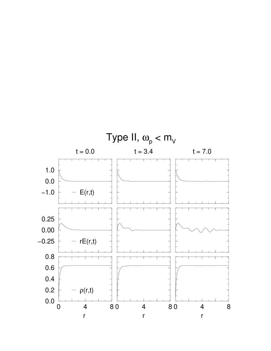
FIG. 8.: Snapshots of the electric field $E$ and monopole field $\rho$ at times of maxima in the on-axis field $E(r=0)$: Type II superconductor, $\omega_{p}<m_{V}$.

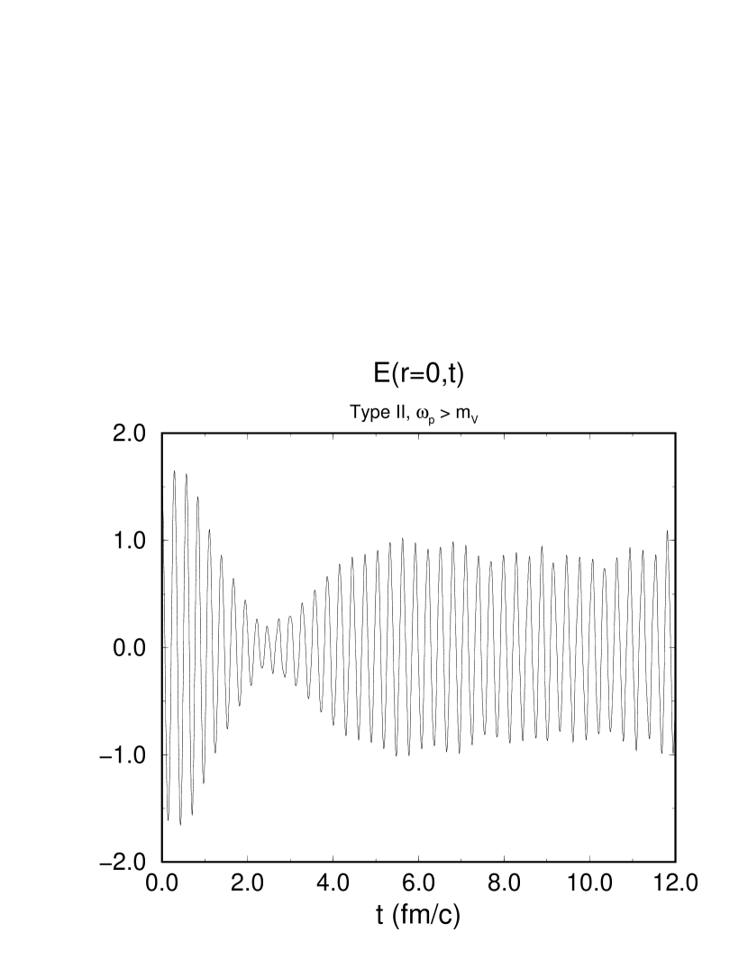
FIG. 9.: Electric field on the $z$ axis, for Type II superconductor with $\omega_{p}>m_{V}$.

FIG. 10.: Snapshots of the electric field $E$ and monopole field $\rho$ at times of maxima in the on-axis field $E(r=0)$: Type II superconductor, $\omega_{p}>m_{V}$.

FIG. 11.: Continuation of fig. 10.

REFERENCES

- [1] A. Chodos, R. L. Jaffe, K. Johnson, C. B. Thorn, V. F. Weisskopf, Phys. Rev. D9, 3471 (1974); K. Johnson and C. B. Thorn, Phys. Rev. D 13, 1934 (1976).
- [2] G. ’t Hooft, Nucl. Phys. B190, 455 (1981).
- [3] S. Mandelstam, Phys. Rep. 23C, 245 (1973).
- [4] A. A. Abrikosov, Zh. Eksp. Teor. Fiz. 32, 1442 (1957) [Sov. Phys. JETP 5, 1174 (1957)].
- [5] G. ’t Hooft, Nucl. Phys. B190, 455 (1981).
- [6] A. S. Kronfeld, M. L. Laursen, G. Schierholz, and U. J. Wiese, Phys. Lett. 198B, 516 (1987); A. S. Kronfeld, G. Schierholz ,and U. J. Wiese, Nucl. Phys. B293, 461 (1987); M. I. Polykarpov, Nucl. Phys. (Proc. Suppl.) 53, 134 (1997); L. Del Debbio, M. Faber, J. Greensite, and Š. Olejník, ibid. 53, 141 (1997), hep-lat/9607053.
-
[7]
E. M. Lifshitz and L. P. Pitaevskii, Statistical Physics,
part 2 (Pergamon Press, New York, 1980);
D. R. Tilley and J. Tilley, Superfluidity and Superconductivity (Adam Hilger, Bristol, 1990). - [8] A. Jevicki and P. Senjanović, Phys. Rev. D11, 860 (1975).
- [9] A. Patkos, Nucl. Phys. B97, 352 (1975).
- [10] J. W. Alcock, M. J. Burfitt and W. N. Cottingham, Nucl. Phys. B226, 299 (1983).
- [11] V.P. Nair and C. Rosenzweig, Nucl. Phys. B250, 729 (1985).
- [12] J. S. Ball and A. Caticha, Phys. Rev. D 37, 524 (1988).
- [13] H. Suganuma, S. Sasaki, and H. Toki, Nucl. Phys. B435, 207 (1995).
- [14] K. Suzuki and H. Toki, Int. J. Mod. Phys. A11, 2677 (1996); S. Sasaki, H. Suganuma, and H. Toki, Prog. Theor. Phys. 94, 373 (1995); I. Ichie, H. Suganuma, and H. Toki, Phys. Rev. D52, 2944 (1995); ibid. 54, 3382 (1996); H. Monden, H. Suganuma, H. Ichie, H. Toki, Phys. Rev. C 57, 2564 (1998); Y. Koma, H. Suganuma, and H. Toki, hep-ph/9902441.
- [15] T. Suzuki, Prog. Theor. Phys. 80, 929 (1988); S. Maedan and T. Suzuki, ibid. 81, 229 (1989); T. Suzuki, ibid. 81, 752 (1989).
- [16] K. Schilling, G.S. Bali and C. Schlichter, hep-lat/9809039. But see D. Diakonov and V. Petrov, hep-lat/9810037.
- [17] A. Casher, H. Neuberger, and S. Nussinov, Phys. Rev. D20, 179 (1979); ibid. 21, 1966 (1980).
- [18] B. Andersson, G. Gustafson, G. Ingelman, and T. Sjostrand, Phys. Rep. 97, 31 (1983); B. Andersson, The Lund Model (Cambridge University Press, Cambridge, 1998).
- [19] T. S. Biró, H. B. Nielsen, and J. Knoll, Nucl. Phys. B245, 449 (1984).
- [20] F. Sauter, Z. Phys. 69, 742 (1931); W. Heisenberg and H. Euler, Z. Phys. 98, 714 (1936); J. Schwinger, Phys. Rev. 82, 664 (1951).
- [21] F. Cooper, J. M. Eisenberg, Y. Kluger, E. Mottola, and B. Svetitsky, Phys. Rev. D48, 190 (1993).
- [22] J.M. Eisenberg, Phys. Rev. D51, 1938 (1995).
- [23] D. Zwanziger, Phys. Rev. D3, 880 (1971); M. Blagojević and P. Senjanović, Phys. Rep. 157, 233 (1988).
- [24] S. Loh, C. Greiner, U. Mosel, and M. H. Thoma, Nucl. Phys. A619, 321 (1997).
- [25] R. Friedberg and T. D. Lee, Phys. Rev. D 15, 1694 (1977); ibid. 16, 1096 (1977); ibid. 18, 2623 (1978).
-
[26]
M. Blagojević and P. Senjanović,
Nucl. Phys. B161, 112 (1979);
M. Blagojević, S. Meljanac, and P. Senjanović, Phys. Rev. D32, 1512 (1985). - [27] A. K. Kerman, T. Matsui, and B. Svetitsky, Phys. Rev. Lett. 56, 219 (1986).
- [28] S. Coleman, in The Unity of the Fundamental Interactions: Proceedings of the International School of Subnuclear Physics (1981: Erice, Italy), ed. Antonino Zichichi (Plenum Press, New York, 1983).
- [29] K.-I. Kondo, Phys. Rev. D 57, 7467 (1998); ibid. 58, 105016 (1998) ;ibid. 58, 105019.