Implications of a new solar system population of neutralinos on indirect detection rates

Abstract:

Recently, a new Solar System population of weakly interacting massive particle (WIMP) dark matter has been proposed to exist. We investigate the implications of this population on indirect signals in neutrino telescopes (due to WIMP annihilations in the Earth) for the case when the WIMP is the lightest neutralino of the MSSM, the minimal supersymmetric extension of the standard model. The velocity distribution and capture rate of this new population is evaluated and the flux of neutrino-induced muons from the center of the Earth in neutrino telescopes is calculated. The strength of the signal is very sensitive to the velocity distribution of the new population. We analytically estimate this distribution using the approximate conservation of the component of the WIMP angular momentum orthogonal to the ecliptic plane. The non-linear problem of combining a fixed capture rate from the standard galactic WIMP population with one rising linearly with time from the new population to obtain the present-day annihilation rate in the Earth is also solved analytically. We show that the effects of the new population can be crucial for masses below around 150 GeV, where enhancements of the predicted muon flux from the center of the Earth by up to a factor of 100 compared to previously published estimates occur. As a result of the new WIMP population, the next generation of neutrino telescopes should be able to probe a much larger region of parameter space in the mass range 60-130 GeV.

1 Introduction

It has been known for almost 15 years that Weakly Interacting Massive Particles (WIMPs) can elastically scatter inside the Sun and Earth, leading to their subsequent capture and annihilation in the cores of these objects, producing an indirect neutrino signature that might be accessible to neutrino telescopes [1]. Recently, however, it has been demonstrated that the scattering process in the Sun can populate orbits which subsequently result in a bound Solar System population of WIMPs [2, 3] and which can be comparable in spectral density, in the region of the Earth, to the Galactic halo WIMP population. This new population consists of WIMPs that have scattered in the outer layers of the Sun and due to perturbations by the other planets (mainly Jupiter) evolve into bound orbits which do not cross the Sun but do cross the Earth’s orbit. This population of WIMPs should have a completely different velocity distribution than halo WIMPs and will thus have quite different capture probabilities in the Earth. The predicted WIMP abundance, and spectrum, relevant for direct detection have been calculated [2, 3]. Here we focus on capture in the Earth, and the predicted indirect neutrino signature. Other studies of solar system populations of WIMPs can be found in [1, 4, 5].

Following [2, 3], we consider here a special WIMP candidate, the neutralino, which arises naturally in supersymmetric extensions of the standard model. We evaluate the capture of neutralinos and the resulting neutrino-induced muon flux within the Minimal Supersymmetric extension of the Standard Model (MSSM) (for a review of neutralino dark matter, see ref. [6]). We find that this flux is sensitively dependent upon the Solar System WIMP velocity distribution, and can exceed by two orders of magnitude that predicted for Galactic halo WIMPs. Although our numerical results apply only to supersymmetric WIMPs, we expect our qualitative conclusions to be generally valid for any WIMP model of dark matter.

2 Definition of the supersymmetric model

We work in the Minimal Supersymmetric Standard Model (MSSM). In general, the MSSM has many free parameters, but with customary assumptions [6] (which do not significantly affect the general results of this paper) we can reduce the number of parameters to seven: the Higgsino mass parameter $\mu$, the gaugino mass parameter $M_{2}$, the ratio of the Higgs vacuum expectation values $\tan\beta$, the mass of the $CP$-odd Higgs boson $m_{A}$, the scalar mass parameter $m_{0}$ and the trilinear soft SUSY-breaking parameters $A_{b}$ and $A_{t}$ for the third generation. In particular, we do not impose any restrictions from supergravity other than gaugino mass unification. We have made some scans in parameter space without the GUT relation $3M_{1}=5M_{2}\tan^{2}\theta_{W}$ for the gaugino mass parameters $M_{1}$ and $M_{2}$. This mainly has the effect of allowing lower neutralino masses to escape the LEP bounds and is not very important for this study. Hence, the GUT relation for $M_{1}$ and $M_{2}$ is kept throughout this paper. For a more detailed definition of the parameters and a full set of Feynman rules, see refs. [7, 8]. Of course we assume $R$-parity conservation, which ensures that the lightest supersymmetric particle is stable and therefore an excellent dark matter candidate. Its relic abundance today is fixed by its freeze-out abundance in the early Universe, which in turn is given by the interplay between the interaction rate and the expansion rate at a temperature around $T\sim m_{\chi}/20$, where $m_{\chi}$ is the neutralino mass (i.e. it is non-relativistic at freeze-out and would act as cold dark matter in structure formation).

The lightest (and, with $R$-parity conservation, stable) supersymmetric particle is in most models the lightest neutralino, which is a superposition of the superpartners of the gauge and Higgs fields,

$$\tilde{\chi}^{0}_{1}=N_{11}\tilde{B}+N_{12}\tilde{W}^{3}+N_{13}\tilde{H}^{0}_{1}+N_{14}\tilde{H}^{0}_{2}\,.$$ (1)

It is convenient to define the gaugino fraction of the lightest neutralino,

$$Z_{g}=|N_{11}|^{2}+|N_{12}|^{2}\,.$$ (2)

For the masses of the neutralinos and charginos we use the one-loop corrections as given in ref. [9] and for the Higgs boson masses we use the leading log two-loop radiative corrections, calculated within the effective potential approach given in ref. [10].

Parameter	$\mu$	$M_{2}$	$\tan\beta$	$m_{A}$	$m_{0}$	$A_{b}/m_{0}$	$A_{t}/m_{0}$
Unit	GeV	GeV	1	GeV	GeV	1	1
Min	-50000	-50000	1.0	0	100	-3	-3
Max	50000	50000	60.0	10000	30000	3	3

Table 1: The ranges of parameter values used in our scans of the MSSM parameter space. Note that several special scans aimed at interesting regions of the parameter space have been performed. In total we have generated approximately $1.4\times 10^{5}$ models which are not excluded by accelerator searches.

We have made extensive scans of the model parameter space, some general and some specialized to interesting regions, where high rates are possible. In total we have made 33 different scans of the parameter space. The scans were done randomly and were mostly distributed logarithmically in the mass parameters and in $\tan\beta$. For some scans the logarithmic scan in $\mu$ and $M_{2}$ was replaced by a logarithmic scan in the more physical parameters $m_{\chi}$ and $Z_{g}/(1-Z_{g})$, where $m_{\chi}$ is the neutralino mass. Combining all the scans, the overall limits of the seven MSSM parameters we use are given in table 1.

We check each model to see if it is excluded by the most recent accelerator constraints, of which the most important ones are the LEP bounds [11] on the lightest chargino mass,

$$m_{\chi_{1}^{+}}>\left\{\begin{array}[]{lcl}91{\rm~{}GeV}&\,,&|m_{\chi_{1}^{+}}-m_{\chi^{0}_{1}}|>4{\rm~{}GeV}\\ 85{\rm~{}GeV}&\,,&{\rm otherwise}\end{array}\right.$$ (3)

and on the lightest Higgs boson mass $m_{H_{2}^{0}}$ (which range from 72.2–88.0 GeV depending on $\sin(\beta-\alpha)$ with $\alpha$ being the Higgs mixing angle) and the constrains from $b\to s\gamma$ [12]. For each allowed model we calculate the relic density of neutralinos $\Omega_{\chi}h^{2}$, where $\Omega_{\chi}$ is the density in units of the critical density and $h$ is the present Hubble constant in units of $100$ km s^-1 Mpc^-1. We use the formalism of ref. [13] for resonant annihilations, threshold effects, and finite widths of unstable particles and we include all two-body tree-level annihilation channels of neutralinos. We also include so-called coannihilation processes in the relic density calculation according to the analysis of Edsjö and Gondolo [7].

Present observations favor $h=0.65\pm 0.1$, and a total matter density $\Omega_{M}=0.3\pm 0.1$, of which baryons may contribute 0.02 to 0.08 [14]. Not to be overly restrictive, we accept $\Omega_{\chi}h^{2}$ in the range from $0.025$ to $1$ as cosmologically interesting. The lower bound is somewhat arbitrary as there may be several different components of non-baryonic dark matter, but we demand that neutralinos are at least as abundant as required to make up the dark halos of galaxies. In principle, neutralinos with $\Omega_{\chi}h^{2}<0.025$ would still be relic particles, but only making up a small fraction of the dark matter of the Universe, so we do not consider this alternative here.

3 Speed distribution of the new neutralino population

The distribution of Solar System WIMPs relevant to terrestrial capture arises from scattering of Galactic halo WIMPs into highly elliptical Solar System orbits, with semi-major axes in the range $a_{\rm earth}<a<2.6a_{\rm earth}$. These are then perturbed by Jupiter and the other planets into orbits which do not intersect the Sun. Analytical methods were used in refs. [2, 3] to estimate the basic features of this distribution. Here we shall relax an approximation (exactly radial orbits) made in refs. [2, 3] and derive an improved analytical estimate of this distribution. We nevertheless expect, because of their origin in Solar scattering, that most of these orbits will be close to radial in the vicinity of the Earth.

In ref. [5], the phase space distribution of WIMPs at the Earth was investigated including the effects of the Earth being deep in the Sun’s potential well. There it was found that even though the velocity distribution of WIMPs at the Earth is different than it would be in free space, both Jupiter, the Earth and Venus will disturb the orbits of these unbound WIMPs into bound orbits that have the same phase space distribution as would be the case in free space. This relies on the fact that the time-scales for transferring WIMPs between these unbound and bound orbits are shorter than the age of the Earth so that an equilibrium occurs. This is valid for low velocities relative to the Earth only (which are the most important ones for capture) and it was found that for some higher-velocity orbits (velocities $\gtrsim$ 27 km/s), the time-scale for filling or depleting these bound orbits is too long. It turns out that the (nearly) radial orbits of interest for this work happen to be in precisely this regime. More precisely, our new population is distributed along a thin vertical “needle”, located within the “unfilled bound orbits” region of fig. 3 of ref. [5], starting at $u=30$ km/s on the left part of the horizontal axis. This is of course an advantage for detection since it means that these WIMPs will stay in these orbits without being much affected by diffusion within the Solar System.

The detection rates we discuss below are very sensitive to the actual form of the velocity distribution, especially at low velocities (with respect to the Earth). The reason for this is easy to understand from simple kinematics. A very heavy WIMP (heavier than iron) which encounters the Earth cannot be stopped by a single encounter if its velocity is large. (And the optical depth for repeated scatterings is very small.) Therefore, it is the strength of the distribution at low energies which determines the capture rate and therefore the muon neutrino rate from the center of the Earth. An exception to the rule of only low velocities being important occurs if the WIMP has a mass which closely matches one of the most abundant elements of the Earth. Then kinematics allows all the kinetic energy of the WIMP to be transferred to a nucleus in a single collision. As we shall discuss in detail below, conservation of the z component of the angular momentum constrains very much the component of the velocity of the WIMPs along the motion of the Earth, and thereby the lowest attainable speed with respect to the Earth. As a consequence, we shall see that only neutralinos of the new population lighter than around 150 GeV will be captured by the Earth.

Let us now turn to the best estimate we can presently make of the velocity distribution, as seen in an Earth frame, of the new neutralino population. In refs. [2, 3], as a first approximation, a model was used where the WIMP orbits were nearly radial (i.e. with a fixed eccentricity, very near $e=1$). Here, we shall go beyond this approximation by taking into account the distribution in the $z$ component of the angular momentum (which will turn out to be the crucial one for our purpose). Let us first define our notation.

In an heliocentric frame, the WIMP phase-space distribution function would read $dN=f({\bf x},{\bf v})\,d^{3}{\bf x}\wedge d^{3}{\bf v}$, where ${\bf x}$ denotes the WIMP heliocentric position and ${\bf v}$ its heliocentric velocity. We could start from $f({\bf x},{\bf v})$, written as a function of the integrals of motion of the WIMP (so that it satisfies Liouville’s equation), to derive the capture rate in the Earth. It is, however, more convenient to take advantage from the start of the simplification brought by the spherical symmetry of the Earth. Let ${\bf u}={\bf v}-{\bf v}_{E}$ denote the incoming velocity (far from the Earth) of the WIMP in an Earth reference frame (here ${\bf v}_{E}$ denotes the heliocentric velocity of the Earth). The WIMP capture rate by the spherically symmetric Earth depends only on the angular average of the velocity distribution, and therefore is a function only of the distribution of “speeds” $u\equiv|{\bf u}|$. We can write the speed distribution of the local WIMP number density as

$$dn(u)=n(a_{1})\,d\,\widehat{n}(u)\,,$$ (4)

where $n(a_{1})$, with $a_{1}\equiv 1AU$ denoting the radius of the Earth’s orbit, is the total space density around the Earth (WIMPs per cm³), and where $d\,\widehat{n}(u)$ is the normalized speed distribution: $\int d\,\widehat{n}(u)=1$. The integrated WIMP space density $n(a_{1})$ has been estimated in refs. [2, 3]. We shall quote the result below when we need it. We focus first on the normalized speed distribution $d\,\widehat{n}(u)$.

At any moment we can introduce an heliocentric spatial reference frame $(x,y,z)$ such that the $x$-axis is in the Sun-Earth radial direction, and the $y$-axis is directed along the orbital motion of the Earth. In this frame

$$u^{2}=({\bf v}-{\bf v}_{E})^{2}={\bf v}^{2}+v_{E}^{2}-2\,v_{E}\,v_{y}\,.$$ (5)

As we are considering a fixed value $r\equiv|{\bf x}|=a_{1}$ of the WIMP radial position, the squared heliocentric velocity ${\bf v}^{2}$ can be expressed in terms of the semi-major axis of the WIMP orbit:

$${\bf v}^{2}(r=a_{1})=v_{E}^{2}\left(2-\frac{a_{1}}{a}\right).$$ (6)

On the other hand, the longitudinal (“along the track”) velocity $v_{y}$ entering eq. (5) can be expressed in terms of the $z$-component $J_{z}$ of the angular momentum of the WIMP, $v_{y}=J_{z}/a_{1}$ (note that the $z$ axis is orthogonal to the ecliptic plane). Finally, the (square of the) local speed of the WIMP can be entirely expressed in terms of the two adiabatic invariants $a$ and $J_{z}$ (i.e. the two Delaunay action variables $L=\sqrt{G_{N}\,M_{\rm Sun}\,a}$ and $H=\sqrt{G_{N}\,M_{\rm Sun}\,a(1-e^{2})}\cos i$ in the notation of ref. [3]):

$$u^{2}=v_{E}^{2}\left(3-\frac{a_{1}}{a}-\frac{2\,J_{z}}{a_{1}\,v_{E}}\right).$$ (7)

We recall that $v_{E}=(G_{N}\,M_{\rm Sun}/a_{1})^{1/2}=27.98$ km s^-1 denotes the Earth orbital speed, and $a_{1}=r_{E}=1\ AU$.

Let us recall from ref. [3] that, to a good approximation, the two WIMP action variables $L$ and $H$ are secularly conserved (modulo some small random-walk-type diffusion caused by near encounters with the inner planets), while the third action variable $G=\sqrt{G_{N}\,M_{\rm Sun}\,a(1-e^{2})}$ will secularly evolve under the influence of planetary perturbations. [The averaged planetary Hamiltonian $\overline{\cal H}_{p}$ (Kozai Hamiltonian) was discussed in section 3 of [3].] The evolution of $G$ means that the eccentricity of the WIMP orbit oscillates between values very near one and smaller values. We see from eq. (7) that these eccentricity oscillations have no effect on the local speed distribution. The latter depends only on the well conserved quantities $L$ and $H$, or $a$ and $J_{z}$. We can then estimate the present speed distribution by means of the initial distribution of $a$ and $J_{z}$. [“Initial” means here at the time when the considered WIMP of the new population exited from the Sun after having been captured by scattering on a nucleus in the outskirts of the Sun.] The initial $z$-component of the WIMP angular momentum was

$$J_{z}^{0}=\sqrt{G_{N}\,M_{\rm Sun}\,a_{0}(1-e_{0})(1+e_{0})}\cos i_{0}\,.$$ (8)

Here, $a_{0}(1-e_{0})$ is the initial perihelion distance which is approximately equal to the (effective) Sun radius $\overline{R}_{S}=0.907\,R_{\rm Sun}$. The remaining factor $1+e_{0}$ can be approximated by 2, so that

$$J_{z}^{0}\simeq\sqrt{2G_{N}\,M_{\rm Sun}\,\overline{R}_{S}}\cos i_{0}\,,$$ (9)

where the cosine of the initial inclination can be (approximately) considered as being a random variable uniformly distributed between $-1$ and $+1$.

Because of the overall (approximate) axial symmetry of the Solar System, we expect the conservation law of $J_{z}$ to be rather accurate: $J_{z}^{\rm now}\simeq J_{z}^{0}$. However, as the nonconservation of $J_{z}$ would have a crucial effect on the capture rate of WIMPs by the Earth (by allowing for lower speeds in an Earth frame, through the last term in eq. (7)) we shall introduce a phenomenological parameter $\lambda$ to parametrize a possible nonconservation of $J_{z}$. More precisely, we shall assume that

$$J_{z}^{\rm now}=\lambda\,J_{z}^{0}\,,$$ (10)

and study not only the “standard” case where $\lambda=1$, but also the case where, say, $\lambda=2$, which corresponds to a 100% violation of the conservation of $J_{z}$. Then, eq. (7) reads

$$u^{2}=v_{E}^{2}\left(3-\frac{a_{1}}{a}-\varepsilon\,\cos i_{0}\right),$$ (11)

where

$$\varepsilon\equiv 2\lambda\ \sqrt{\frac{2\,\overline{R}_{S}}{a_{1}}}\simeq 0.18377\,\lambda\,.$$ (12)

Eq. (11) tells us that the distribution function of the squared speed $u^{2}$ is obtained by taking the convolution between the distribution of the variable $b\equiv a_{1}/a$ (which is essentially the WIMP heliocentric energy) and the (uniform) distribution of the variable $c\equiv\varepsilon\,\cos i_{0}$. If we denote $b^{\prime}\equiv b+\varepsilon\,\cos i_{0}$, the distribution $\varphi^{\prime}(b^{\prime})\,db^{\prime}$ of $b^{\prime}$ is given in terms of the distribution $\varphi(b)\,db$ of $b\equiv a_{1}/a$ by

$$\varphi^{\prime}(b^{\prime})=\frac{1}{2\,\varepsilon}\int_{-\varepsilon}^{\varepsilon}\varphi(b^{\prime}-\xi)\,d\xi\,.$$ (13)

The normalized distribution $\varphi(b)\,db$ (with $\int\varphi(b)\,db=1$) has been derived in ref. [3]. It is written in eq. (6.7) there, in terms of the related variable $x=2a/a_{1}=2/b$. (Ref. [3] made the approximation of nearly radial orbits in deriving eq. (6.7), but this approximation is not crucial for our present purpose. The crucial new feature for the present work is the allowance for the along-the-track term proportional to $J_{z}$ in eq. (7) which is the only one which can significantly affect neutralino capture by the Earth.) Transcribing eq. (6.7) of [3] in terms of the variable $b=2/x$ yields

$$\varphi(b)\,db=N_{b}\ \frac{db}{b^{0.6}\,(2-b)^{1/2}}\ \theta\left(b-\frac{1}{2.6}\right)\,\theta(2-b)\,,$$ (14)

with the normalization constant

$$N_{b}=\frac{2^{0.1}}{I_{n}(5.2)}=0.456579\,.$$ (15)

Here, as above, $\theta(x)$ denotes the step function ($\theta(x)=1$ if $x>0$, $\theta(x)=0$ if $x<0$).

Eq. (13) then gives the distribution in $b^{\prime}$, or equivalently in the scaled squared speed

$$U\equiv\widehat{u}^{2}\equiv\left(\frac{u}{v_{E}}\right)^{2}=3-b^{\prime}=3-b-\varepsilon\,\cos i_{0}\,.$$ (16)

Before the smearing of eq. (13) (due to the convolution with the $J_{z}$-distribution) the original distribution $\varphi(b)\,db$ of eq. (14) featured both a cut-off at $b_{1}=a_{1}/a=2$ and a cut-off at $b_{2}=1/2.6$. The former cut-off corresponds to a lower-velocity cut-off at $u=v_{E}(3-b_{1})^{1/2}=v_{E}=29.78$ km s^-1. (It corresponds to radial orbits which barely reach up to the Earth orbit.) In our present refined treatment, where we take into account the along-the-track motion linked to the distribution in $J_{z}$, this lower-velocity cut-off will be shifted to a lower value (coming from a positive $J_{z}$ in eq. (7)). For capture by the Earth (which has a small escape velocity, ranging between about 11 and 15 km s^-1) the low-velocity part of the speed distribution is the only one to play a crucial role. We can take advantage of this fact to derive a simplified analytical expression of the speed distribution $d\,\widehat{n}(U)=\varphi^{\prime}(3-U)\,dU=\varphi^{\prime}(b^{\prime})\,db^{\prime}$. Indeed, we can approximate the smearing, eq. (13), as acting only on the crucial low-velocity cut-off factor $\theta(2-b)/(2-b)^{1/2}$ in eq. (14). The smearing of the smoothly varying factor $1/b^{0.6}$ would only introduce a small fractional correction of order $\varepsilon^{2}\sim 3$%. With this approximation the smearing integral of eq. (13) can be explicitly computed. The final result for the speed distribution reads

$$d\,\widehat{n}=N^{\prime}_{\varepsilon}\,f_{\varepsilon}(U)\,dU=N^{\prime}_{\varepsilon}\,f_{\varepsilon}(\widehat{u}^{2})\,2\,\widehat{u}\,d\,\widehat{u}\,,$$ (17)

where we recall that $U\equiv\widehat{u}^{2}\equiv(u/v_{E})^{2}$, where $N^{\prime}_{\varepsilon}$ is a normalization constant (equal to $N_{b}$, eq. (15), modulo ${\cal O}(\varepsilon^{2})$ fractional corrections) and where $f_{\varepsilon}(U)$ is explicitly given by

$$f_{\varepsilon}(U)=\frac{\theta\,(U_{\rm max}-U)}{(3-U)^{0.6}}\ \frac{1}{\varepsilon}\left[\sqrt{U-1+\varepsilon}\ \theta\,(U-1+\varepsilon)-\sqrt{U-1-\varepsilon}\ \theta\,(U-1-\varepsilon)\right]\,.$$ (18)

Here $U_{\rm max}=3-1/2.6\simeq 2.6154$ is the upper cut-off, and $\varepsilon$ is given by eq. (12) (with $\lambda=1$ being our standard estimate, and $\lambda=2$ being an extreme phenomenological possibility). Note that the speed distribution extends only between a minimum cut-off at

$$u_{\rm min}=v_{E}\ \sqrt{1-\varepsilon}$$ (19)

and a maximum at $u_{\rm max}=v_{E}\ \sqrt{U_{\rm max}}\simeq 48.16$ km s^-1. (The exact maximum cut-off given by eq. (13) is modified by ${\cal O}(\varepsilon)$ terms, but this modification is unimportant for our present purpose.) The numerical value of the lower speed cut-off, eq. (19), is 26.905 km s^-1 for the standard case $\lambda=1$, and 23.683 km s^-1 for the extreme case $\lambda=2$. The precise value of this lower speed cut-off is important because it translates into an upper cut-off in the masses of the WIMPs that can be captured by the Earth. Indeed, as will be recalled below, the kinematics of the maximum energy loss in the collision of a WIMP of mass $m_{X}$ with a nucleus of mass $m_{A}$ located at radius $r$ in the Earth (with local escape velocity $v_{\rm esc}(r)$) is such that capture is only possible if

$$\beta_{-}^{A}\equiv\frac{4\,m_{X}\,m_{A}}{(m_{X}-m_{A})^{2}}\geq\left(\frac{u_{\rm min}}{v_{\rm esc}(r)}\right)^{2}\,.$$ (20)

This implies the following upper limit on the mass of a WIMP capturable by the Earth

$$m_{X}\leq\left(1+2w+2\,\sqrt{w^{2}+w}\right)m_{A}\,,$$ (21)

where we denoted $w\equiv(v_{\rm esc}(r)/u_{\rm min})^{2}$. The highest capturable mass is reached when the WIMP scatters on an iron nucleus ($m_{A}=m_{\rm Fe}\simeq 52$ GeV) located at the center of the Earth (where $v_{\rm esc}(0)\simeq 15$ km s^-1). In our standard case ($\lambda=1$) where $u_{\rm min}\simeq 26.905$ km s^-1 this yields the upper limit

$$m_{X}\leq 2.90\,m_{\rm Fe}\simeq 150\,{\rm GeV}\,,$$ (22)

on the other hand in the case $\lambda=2$ the limit is shifted to about 170 GeV.

4 Overdensity of the new population

We follow the notation of [2, 3] and write the contribution from this new population of WIMPs to the usual halo WIMP density as

$$\delta_{E}\equiv\frac{n(a_{1})}{n_{X}}\equiv\frac{\hbox{(secondary) WIMP density at the Earth}}{\hbox{halo WIMP density at infinity}}\,,$$ (23)

where

$$\delta_{E}=\frac{5.44\times 10^{36}}{(v_{o}/220\,{\rm km\,s}^{-1})}\times g_{\rm tot}\,{\rm GeV}\,{\rm cm}^{-2}=\frac{0.212}{(v_{o}/220\,{\rm km\,s}^{-1})}\,g_{\rm tot}^{(-10)}\,.$$ (24)

Here, $g_{\rm tot}^{(-10)}\equiv 10^{10}\,g_{\rm tot}({\rm GeV})^{3}$, and $g_{\rm tot}={\sum_{A}}\,(f_{A}/m_{A})\,\sigma_{A}\,K_{A}^{s}$, where $f_{A}$ is the mass fraction of element $A$ in the Sun, and $K_{A}^{s}$ is the surface value of the capture function on the element of mass number $A$ in the Sun according to eq. (2.20) in ref. [3].

The scattering rate of WIMPs in the outer layers of the Sun (which causes the fast halo WIMPs to lose enough energy to enter bound orbits close to the Earth’s orbit) is proportional to $\sigma_{A}K_{A}^{s}$, which can be calculated once the parameters of the SUSY WIMP in question are fixed. (For the elemental abundances in the Sun, we use the compilation of Bahcall and Pinsonneault [15].)

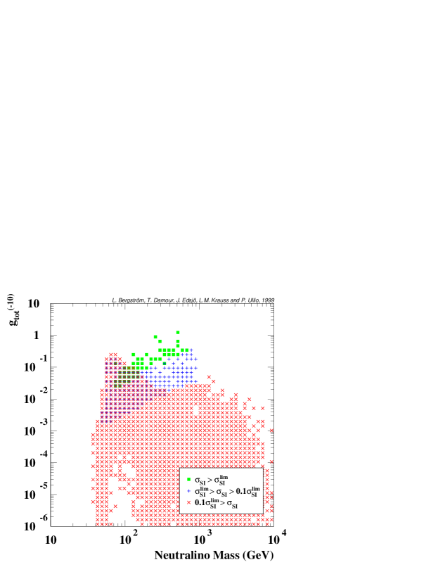
Figure 1: The value of the parameter $g_{{\rm tot}}^{(-10)}$, which is related to the scattering probability near the Solar surface, as a function of neutralino mass. The different symbols represent different ranges for the spin-independent cross section, where $\sigma_{SI}^{\rm lim}$ represents the most stringent claimed upper limit on this cross section for an assumed halo density of 0.3 GeV/cm³, given in [16] (see text for a discussion).

In fig. 1 we display the values of $g_{\rm tot}^{(-10)}$ versus neutralino mass for our set of supersymmetric models. As can be seen, in some cases values approaching or even exceeding unity can be obtained (confirming the results of [2, 3]). The spread is very large, however, and some models give orders of magnitude smaller values. As would be expected, the models with the highest values of $g_{\rm tot}^{(-10)}$ are the same models which give high scattering rates in direct detection experiments (the value of the local halo density is assumed to be 0.3 GeV cm^-3). This can be seen by the coding of the displayed points in terms of one claimed limit [16] on the spin-independent scattering cross section.

Note that the highest values of $g_{\rm tot}^{(-10)}$ allowed by this claimed limit on the scattering rates is $g_{\rm tot~{}max}^{(-10)}\simeq 0.4$. Such values imply only a rather modest (but not negligible, and important as independent check) effect of the new population in direct experiments (see refs. [2, 3]). On the other hand, we shall see below that they can imply a large effect on indirect detection rates.

5 Capture rate of WIMPs by the Earth

The total space density of WIMPs, per speed element, in the vicinity of the Earth reads

$$\begin{array}[b]{rcl}dn_{X}^{\rm tot}=dn_{X}^{\rm old}+dn_{X}^{\rm new}&=&n_{X}\,d\,\widehat{n}^{\rm old}(u)+n^{\rm new}(a_{1})\,d\,\widehat{n}^{\rm new}(u)\\ &=&n_{X}\left[d\,\widehat{n}^{\rm old}(u)+\delta_{E}\,d\,\widehat{n}^{\rm new}(u)\right].\end{array}$$ (25)

The “old” distribution $d\,\widehat{n}^{\rm old}(u)$ can, to a good approximation [5], be considered to be simply the incoming Galactic one, shifted to the frame of the moving Earth. The “new” (secondary) distribution $d\,\widehat{n}^{\rm new}(u)$ is that defined by eq. (17) above. The present overdensity ratio $\delta_{E}$ is that discussed in section 4 above. Let us now write down the capture rate of WIMPs by the Earth [17, 18]. We shall utilize the result of Gould [18], using the notation of ref. [3]. As said above, we work here with the angle-averaged speed distribution, which reads, in the notation of ref. [3], $dn_{X}(u)=4\pi\,u^{2}\,du\,\overline{f}_{\infty}(u)$. Using eqs. (2.20)–(2.22) of ref. [3], considered for $J_{\rm min}=0$, we get for the capture rate on element $A$:

$$d\dot{N}_{A}=\frac{1}{\beta_{+}^{A}}\ d^{3}{\bf x}\,n_{A}(r)\,\sigma_{A}\ \frac{dn_{X}(u)}{u}\ \exp\left[-\frac{m_{X}}{2Q_{A}}\ (u^{2}+\alpha)\right]\,\theta_{\alpha}\,d\alpha\,,$$ (26)

with

$$\theta_{\alpha}\equiv\theta\left[\beta_{-}^{A}\left(v_{\rm esc}^{2}(r)-\frac{\alpha}{\beta_{+}^{A}}\right)-u^{2}\right].$$ (27)

Here

$$\beta_{\pm}^{A}\equiv\frac{4\,m_{X}\,m_{A}}{(m_{X}\pm m_{A})^{2}}\,,$$ (28)

$\sigma_{A}$ would be the total scattering cross section on nucleus $m_{A}$ in absence of the form factor $F_{A}^{2}(Q)=\exp\,(-Q/Q_{A})$, with $Q=E_{\rm before}-E_{\rm after}$ denoting the energy loss and $Q_{A}$ the standard value of the coherence energy [6], recalled in eq. (2.28) of [3], and $\alpha$ is linked to the semi-major axis of the WIMP, after capture by the Earth, by

$$\alpha\equiv\frac{G_{N}\,M_{\rm Earth}}{a}\,.$$ (29)

Note that we work here in a geocentric frame (with ${\bf u}={\bf v}_{X}^{\infty}-{\bf v}_{E}$). The differential capture rate, eq. (26), must be integrated over $\alpha$ and the volume of the Earth, and must be summed over the label $A$ denoting the various elements in the Earth. The integral over $\alpha$ is limited by the theta function $\theta_{\alpha}$, eq. (27), and by the fact that $\alpha$ must be positive (which expresses the fact that the WIMP lost enough energy by scattering on element $A$ to end up being bound to the Earth). These two constraints restrict the range of variation of $\alpha$ to $0<\alpha<\alpha_{m}(r,u)$, with

$$\alpha_{m}(r,u)=\beta_{+}^{A}\,v_{\rm esc}^{2}(r)-\frac{\beta_{+}^{A}}{\beta_{-}^{A}}\,u^{2}\,,$$ (30)

and imply the presence of a remaining theta function restricting the allowed values of $u$:

$$\theta_{u}\equiv\theta\,(\beta_{-}^{A}\,v_{\rm esc}^{2}(r)-u^{2})\,.$$ (31)

Finally, integration over $\alpha$ (followed by integration over $d^{3}{\bf x}$ and $dn_{X}(u)$, and summation over $A$) leads to a total capture rate

$$\begin{array}[]{rcl}C=\sum_{A}\dot{N}_{A}&=&\displaystyle\sum_{A}\frac{2Q_{A}}{\beta_{+}^{A}\,m_{X}}\int d^{3}{\bf x}\,n_{A}(r)\,\sigma_{A}\,\frac{dn_{X}(u)}{u}\times\\[8.61108pt] &&{}\times\left[\exp\left(-\frac{m_{X}}{2Q_{A}}\,u^{2}\right)-\exp\left(-\frac{m_{X}}{2Q_{A}}\,\beta_{+}^{A}(v_{\rm esc}^{2}(r)+u^{2})\right)\right]\theta_{u}\,.\end{array}$$ (32)

Region	$f_{\rm O}$	$f_{\rm Mg}$	$f_{\rm Si}$	$f_{\rm Fe}$
$r<3488$ km	0.05	0	0	0.90
3488 km $<r<$ 6378 km	0.44	0.23	0.21	0.059

Table 2: The mass fractions, $f_{i}$ of various elements in the Earth. Data from ref. [19].

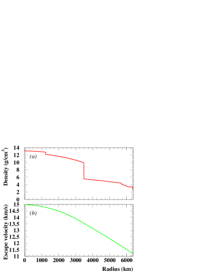
Figure 2: Density (a), and escape velocity (b), as functions of the distance from the center of the Earth.

This capture rate is a linear functional of the WIMP spectrum $dn_{X}(u)$. Therefore the decomposition, eq. (25), implies a corresponding linear decomposition of the capture rate

$$C^{\rm tot}=C^{\rm old}+C^{\rm new}\,.$$ (33)

To evaluate $C^{\rm new}$ we have to perform the integral in eq. (32) explicitly. Available analytical results in the literature do not apply since they assume aMaxwell-Boltzmann velocity distribu-tion. Since we have spherical symmetry, we are left with a double integral, one over the distance from the Earth’s center, $r$, and one over the velocity $u$. For the composition and density of the Earth as a function of $r$ we use the distributions given in ref. [19]. From the density distribution, we can calculate the gravitational potential as a function of $r$ and hence the escape velocity $v_{\rm esc}(r)$. The density and escape velocity as a function of $r$ are given in fig. 2. In table 2 we show the mass fraction of the (for our purpose) most important elements for different regions in the Earth.

6 Neutralino annihilation rate in the Earth

Let $N(t)$ be the total number of neutralinos trapped, at time $t$, in the core of the Earth. The annihilation rate of neutralino pairs can be written as

$$\Gamma_{a}(t)=\frac{1}{2}\ C_{a}\,N^{2}(t)\,.$$ (34)

The evolution of $N(t)$ is the result of the competition between capture and annihilation:

$$\frac{dN}{dt}=C^{\rm tot}(t)-C_{a}\,N^{2}$$ (35)

(the factor 2 difference in the annihilation terms in eqs. (34) and (35) comes from the fact that neutralinos annihilate in pairs). The constant $C_{a}$ entering equations (34) and (35) is linked to the annihilation cross-section $\sigma_{a}$, and to some effective volumes $V_{j}$, $j=1,2$, taking into account the quasi-thermal distribution of neutralinos in the Earth core:

$$C_{a}=\langle\sigma_{a}\,v\rangle\,\frac{V_{2}}{V_{1}^{2}}\,,$$ (36)

$$V_{j}\simeq 2.3\times 10^{25}\,\left(\frac{j\,m_{X}}{10\,{\rm GeV}}\right)^{-3/2}\,{\rm cm}^{3}\,.$$ (37)

Usually, the capture rate $C$ in eq. (35) is time-independent, being given by the “old”, Galactic WIMP population: $C^{\rm usual}=C^{\rm old}={\rm const}$. In that case, eq. (35) can be simply solved by separating the two variables $N$ and $t$, i.e.

$$t=\int dt=\int\frac{d\,N}{C^{\rm old}-C_{a}\,N^{2}}\,.$$ (38)

This yields for the standard, “old” annihilation rate

$$\Gamma_{a}^{\rm old}=\frac{1}{2}\ C_{a}\,N^{2}=\frac{1}{2}\ C^{\rm old}\,\tanh^{2}\,(\gamma\,t)\,,$$ (39)

with

$$\gamma\equiv(C^{\rm old}\,C_{a})^{1/2}\,.$$ (40)

In the case considered here, where capture comes both from the direct Galactic population and from the secondary population discussed in refs. [2, 3], the total capture rate increases linearly with time, because of the linear-in-time build up of the new population:

$$C^{\rm tot}(t)=C^{\rm old}+\dot{C}\,t\,,$$ (41)

where

$$\dot{C}=\frac{C^{\rm new}}{t_{S}}\,.$$ (42)

Here, $C^{\rm new}$ is the present value of the capture rate of the new population (that discussed in the previous section which assumed an overdensity $\delta_{E}$ built up over the full time $t_{S}$) and $t_{S}=4.5$ Gyr is the build up time, i.e. the lifetime of the Solar System.

Note that the problem of determining the total, present annihilation rate, in presence of the new population, is a non-linear one. The answer cannot be simply split as the effect of the old population, plus the effect of the new one. The differential equation to be solved, eq. (35) with eq. (41), is a Riccati equation. In general, such an equation cannot be solved analytically. However, in the present case (corresponding to the restricted type of equations originally discussed by Riccati), the problem can be solved in terms of Airy functions. To do that let us first scale the variables to simplify the Riccati equation. Let us introduce the reduced variables $x$ and $y$ by posing

$$C^{\rm tot}(t)=C^{\rm old}+\dot{C}\,t\equiv\alpha\,x\,,\qquad N\equiv\beta\,y\,,$$ (43)

where

$$\alpha=\dot{C}^{2/3}\,C_{a}^{-1/3}\,,\qquad\beta=\dot{C}^{1/3}\,C_{a}^{-2/3}$$ (44)

(the notation $\alpha$ here should not be confused with our unrelated previous use of this letter). In terms of $x$ and $y$ the evolution equation (35) reads simply

$$\frac{dy}{dx}+y^{2}=x\,.$$ (45)

If we now introduce a new variable $u(x)$ by posing $y(x)=(du/dx)/u$ (this use of the letter $u$ should not be confused with the notation above for the speed with respect to the Earth), eq. (45) becomes the Airy equation:

$$\frac{d^{2}\,u}{d\,x^{2}}=x\,u\,.$$ (46)

The general solution of (46) reads $u(x)=a\,{\rm Ai}\,(x)+b\,{\rm Bi}\,(x)$, where ${\rm Ai}\,(x)$ is the usual Airy function (decreasing for $x\rightarrow+\infty$) and ${\rm Bi}\,(x)$ the complementary solution (increasing as $x\rightarrow+\infty$). The boundary condition of our problem is that $y$ vanishes when $x$ takes it initial (positive) value

$$x_{i}=\frac{C^{\rm old}}{\alpha}$$ (47)

(corresponding to $t=0$). We are then interested in the final value $y_{f}=y(x_{f})$ of $y$ corresponding to the final (present) value of $x$:

$$x_{f}=\frac{C^{\rm tot}\,(t_{S})}{\alpha}=\frac{C^{\rm old}+\dot{C}\,t_{S}}{\alpha}\,.$$ (48)

This final value is given by

$$y_{f}=\frac{{\rm Ai}^{\prime}(x_{f})\,{\rm Bi}^{\prime}(x_{i})-{\rm Bi}^{\prime}(x_{f})\,{\rm Ai}^{\prime}(x_{i})}{{\rm Ai}(x_{f})\,{\rm Bi}^{\prime}(x_{i})-{\rm Bi}(x_{f})\,{\rm Ai}^{\prime}(x_{i})}\,.$$ (49)

In terms of $y_{f}$ the total, present annihilation rate reads

$$\Gamma_{a}^{\rm tot}(t_{S})=\frac{1}{2}\ \alpha\,y_{f}^{2}\,.$$ (50)

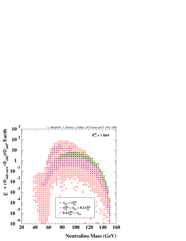
Figure 3: The enhancement factor, eq. (52), as a function of the neutralino mass. The points are symbol coded according to whether they exceed the claimed direct detection bound $\sigma_{SI}$ [16] from the Dama experiment (squares), give direct detection rates within a factor of 10 of those limits (pluses) or give rates more than 10 times smaller than these limits (crosses).

It is useful to consider also the amplification factor ${\cal A}$ brought by the new population, i.e. the ratio

$${\cal A}\equiv 1+{\cal E}\equiv\frac{\Gamma_{a}^{\rm tot}(t_{S})}{\Gamma_{a}^{\rm old}}=\frac{\alpha\,y_{f}^{2}}{C^{\rm old}\,\tanh^{2}\,(\gamma\,t_{S})}\,,$$ (51)

where we have also defined the enhancement factor ${\cal E}\equiv{\cal A}-1$. Note that since the muon flux is directly proportional to the annihilation rate, $\Phi_{\mu}=k\;\Gamma_{a}$, with $k$ depending on the neutralino mass and the ‘hardness’ of the annihilation spectrum, the enhancement factor reads

$${\cal E}=\frac{\Gamma_{a}^{\rm tot}-\Gamma_{a}^{\rm old}}{\Gamma_{a}^{\rm old}}=\frac{\Phi_{\mu}^{\rm old+new}-\Phi_{\mu}^{\rm old}}{\Phi_{\mu}^{\rm old}}\,.$$ (52)

In fig. 3 the enhancement factor for our set of MSSM models is shown against the neutralino mass. As anticipated, the amplification mechanism is only operative for masses smaller than around 150 GeV. Also, for small masses (less than around 60 GeV) the enhancement is relatively small. This is due to a combination of factors, one being that an important contributor to the scattering in the Sun which gives rise to the radial, “planetary” orbits is iron (in fact, it is important also for the capture in the Earth), and for WIMP masses smaller than iron the momentum transfer is less effective. In the WIMP mass region between 60 and 130 GeV, on the other hand, enhancements up to a factor of 100 are possible. This can potentially be very important for the discovery potential for dark matter of neutrino telescopes.

The points in the figure are symbol-coded according to what direct detection rates they correspond to. In particular, the squares indicate neutralino models which exceed the claimed Dama experiment upper limit [16], assuming a halo WIMP density of 0.3 GeV/cm³. In computing the limits from Dama we have included the effects of the new population, but because of the low velocities their effect on present-day detectors with their relatively high recoil energy thresholds is quite small, and in fact hardly visible in our figures.

7 Muon fluxes

Figure 4: The muon flux including both the old and the new population versus the flux obtained if only the old contribution is included. The points are symbol coded according to whether they exceed the claimed direct detection bound $\sigma_{SI}$ [16] from the Dama experiment (squares), give direct detection rates within a factor of 10 of those limits (pluses) or give rates more than 10 times smaller than these limits (crosses).

We calculate the resulting neutrino-induced muon fluxes essentially as described in [20]. The decay and/or hadronization of the annihilation products as well as the neutrino interactions are simulated with Pythia 6.115 [21]. All two-body annihilation final states (at tree level) are included as well as the 1-loop induced 2 gluon and $Z$ gluon. We use a value of $0.3$ GeV/cm³ for the local neutralino mass density (leaving a study of the change in our analysis caused by variations in this and other astrophysical parameters to future work).

We compare the predicted rates with the present experimental upper bound, where we have taken the Baksan results [22] as a representative (the MACRO [23] limits are very similar). The muon threshold is set to 1 GeV. In fig. 4 we show our predicted total muon rates from the direction of the center of the Earth, compared to the rates from the “old” population alone. (Note, that due to the non-linearity of the rate equations, one cannot just sum the contributions of the “new” flux and the “old” flux separately.) As can be seen, enhancements between one and two orders of magnitude are frequent (even though the enhancement for the models with the highest predicted absolute flux is generally somewhat smaller).

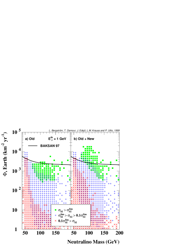
Figure 5: The muon flux obtained from a) only the old population and b) both the old and the new population of WIMPs. The points are symbol coded according to whether they exceed the claimed direct detection bound $\sigma_{SI}$ [16] from the Dama experiment (squares), give direct detection rates within a factor of 10 of those limits (pluses) or give rates more than 10 times smaller than these limits (crosses).

In fig. 5 we show the predicted absolute fluxes against neutralino mass for our sample of models, without and with the new population. The Baksan limit is shown as the nearly horizontal line. As can be seen, the effect on this scatter plot of the new population is striking. Many models around 60–130 GeV have been boosted up to higher fluxes. Several are now above the Baksan limit and others are within detectability in the near future. Around 80 GeV, the increase in flux for models with high fluxes can be as high as a factor of 10 (for low flux models, the increase can be even higher as seen already in fig. 4). One may note that some of the models previously thought to be allowed by Baksan but above the claimed Dama bound, should really be considered as ruled out by Baksan with even greater confidence.

We have investigated the composition of the neutralinos that cause the largest enhancement of the muon flux and that at the same time have high absolute fluxes. We find that they are generally of mixed type (neither very pure Higgsino nor gaugino), and that the biggest enhancements occur for neutralinos which simultaneously have large spin-dependent and spin-independent cross sections. We interpret this as being due to the fact that a large spin-dependent cross section implies efficient scattering on hydrogen in the Sun, whereas a large spin-independent cross section is necessary for capture in the Earth (which is composed of spinless nuclei). The highest fluxes also occur for rather light masses of the CP-odd Higgs boson, $m_{H_{3}^{0}}\lesssim 150$ GeV.

In future experiments, it may be realistic to reach a sensitivity of the order of a few events per km² per year, covering most of the area in the flux versus mass diagram in fig. 5. It is obvious that the enhancements found in this work may be crucial if, for instance, the uncorrected rate would fall just below this value. (It is to be reminded that a priori, we have no knowledge whatsoever about which model, if any, would represent “the world” in our scans.)

The correlation between signals from the Earth and the Sun have also been investigated. Even without this new population, there are models for which the flux from the Earth is higher than that from the Sun, but including this new population, we find many more models (at 60–130 GeV) for which it is more advantageous to look at the Earth than the Sun.

We have also made runs with the angular momentum parameter $\lambda=2$. The results are very similar, and we do not display them here. The main effect is a shift of the kinematical cut-off at 150 GeV to around 170 GeV, and an increased muon rate by up to 50 % in some cases.

8 Conclusions

We have investigated the contribution from a new population of WIMPs coming from WIMPs that have scattered in the outskirts of the Sun and (due to small perturbations by the other planets) are confined to nearly radial orbits reaching out to the Earth.

We find that even for the conservative case when $\lambda=1$ (i.e. the $z$ component of the angular momentum is conserved), we can get enhancements of up to a factor of 100 when the neutralino mass is less than around 150 GeV.

For the mass range of 60–130 GeV some models can already be ruled out on the basis of existing data. The next generation of detectors should be able to probe a much larger region of parameter space in this mass range than would otherwise be possible.

As a result of this new WIMP population, for certain models with WIMPs in the mass range 60–130 GeV, there can be an even greater advantage than before in looking for the indirect signal from the Earth rather than from the Sun.

Whether enhanced annihilations in the Earth for larger WIMP masses might be possible depends on knowing the precise details of the Solar System WIMP velocity distribution, which will await further numerical work on the evolution of Solar System WIMPs.