NLL Corrections for B-Meson Radiative Exclusive Decays
H. H. Asatryan^a, H. M. Asatrian^a, D. Wyler^b

^aYerevan Physics Institute, Alikhanyan Br., 375036-Yerevan, Armenia

^b Institute for Theoretical Physics, University of Zürich, Zürich, Switzerland

Abstract

We calculate the next-to-leading corrections to the branching ratio of exclusive $B\to K^{*}\gamma$ decay. The renormalization scale dependence is reduced compared to the leading logarithmic result but there remains a dependence on a cutoff parameter of the hadronic model. The calculated corrections increase the predicted branching ratio by about 10%, but it remains in agreement with the experimental value.

1 Introduction

The rare neutral flavor changing decays of B-meson are generally considered a good testing ground for new physics [1]. The inclusive decay $b\to s\gamma$ has therefore received intensive experimental [2] and theoretical attention [3]-[11]. In particular, the next-to-leading order calculation for the standard model strongly improved the theoretical uncertainties, most notably the scale dependence of the perturbative calculation.

The calculation of the decay rates for the corresponding exclusive decays such as $B\to K^{*}\gamma$ [12] is usually much more complex because of bound state effects (for a recent work, see for instance [13]). But they are easier to observe, and so it is also of interest to calculate their branching ratios and direct CP asymmetries to the highest possible precision. In this paper we consider the branching ratio for $B\to K^{*}\gamma$ in the next-to-leading logarithmic approximation. The decay $B\to\rho\gamma$ can in principle be treated in the same way, but there are several additional contributions which require new methods.

In [14], the $B\to\rho\gamma$ and $B\to K^{*}\gamma$ branching ratios and rate asymmetries were investigated in the leading logarithmic approximation within a simple meson model. Although this model does not give completely correct results (in particular the ratio of the semileptonic $\pi$ and $\rho$ decays), we will also use it in this work, because of its simplicity.

As usual, the basis of the calculation is the effective Hamiltonian which we record here for completeness. For $B\to K^{*}\gamma$ decay it has the form [14]

$${\cal H}_{eff}=-\frac{4G_{F}}{\sqrt{2}}\left\{\Sigma_{i}v_{t}C_{i}(\mu)O_{i}(\mu)-v_{u}\left[C_{1}(\mu)(O_{1u}(\mu)-O_{1}(\mu))+C_{2}(\mu)(O_{{2u}}(\mu)-O_{2}(\mu))\right]\right\},$$ (1)

where $v_{a}=V_{tb}V_{as}^{*}$, a=u,c,t, i=1,2,…8. For the decay $B\to\rho\gamma$ one must replace $v_{a}$ by $v_{a}^{{}^{\prime}}$, with $v_{a}^{{}^{\prime}}=V_{tb}V_{ad}^{*}$. The operators $O_{i}$ can be found in many places [8, 15, 16].

2 The bound state model

As mentioned, we will use a simple model for the mesons to take into account the bound state effects [14, 17] (for other approaches, see [18],[19]). The B and the $K^{*}$ are described by two constituents: $B=(b,\bar{q})$, $K^{*}=(s,\bar{q})$. The sum of the four momenta of the constituents equals that of the bound state. The mass of the spectator antiquarks is taken to be zero and the b-quark mass becomes momentum dependent:

$$m_{b}=\sqrt{m_{B}^{2}-2p_{B}p_{q}},$$ (2)

where $p_{B}$ and $p_{q}$ are the four momenta of the B-meson and spectator quark, respectively. The momentum $p_{q}$ in the B-meson rest frame is restricted to

$$|p_{q}|=E<m_{B}/2.$$ (3)

The B meson is represented by a matrix $\Psi_{B}$

$$\Psi_{B}=C_{B}\int\frac{d^{3}p_{q}}{2E_{q}(2\pi)^{3}}\sqrt{\frac{m_{B}}{2(m_{B}^{2}-p_{B}p_{q})}}\phi_{B}(|p_{B}p_{q}|/m_{B})\Sigma_{b}\times\frac{1}{\sqrt{N}}1_{N}$$

$$\Sigma_{B}=-(\hat{p}_{b}+m_{b})\gamma_{5}\hat{p}_{q},\hskip 28.45274pt\phi_{B}(p)=\exp(-p^{2}/(2p_{F}^{2})),$$ (4)

where $C_{B}$ is a normalization factor and $p_{F}$ is fixed in such a way that one obtains the correct value of B-meson decay constant $f_{B}$. The ’hat’ symbol stands for the usual ’slash’.

The final state vector meson $K^{*}$ is represented by two constituents with parallel momenta $p_{s}=yp_{V}$, $p_{q}=(1-y)p_{V}$. In most cases its mass and that of the constituent $s$ quark can be neglected (see however the discussion of that point in section 4). It is described by the matrix

$$\Psi_{V}=C_{V}\int_{0}^{1}dy\phi_{V}(y)\Sigma_{V}\times\frac{1}{\sqrt{N}}1_{N},\hskip 28.45274ptC_{V}=f_{V}/(4\sqrt{N})$$

$$\Sigma_{V}=\lim_{m_{V}\to 0}\hat{\epsilon}_{V}^{*}(\hat{p}_{V}+m_{V}),\hskip 28.45274pt\phi_{V}(y)=6y(1-y)(1+\cdot\cdot\cdot),$$ (5)

where $\phi_{V}(y)$ for $V=K^{*},\rho$ are given by [19, 20]:

$$\phi_{K^{*}}(y) = 6y(1-y)(1+0.57(2y-1)-1.35((2y-1)^{2}-1/5)+$$ (6)

$$+ 0.46(7(2y-1)^{3}/3-(2y-1)))$$

$$\phi_{\rho}(y) = 6y(1-y)(1-0.85((2y-1)^{2}-1/5)).$$

The $B\to K^{*}\gamma$ transition matrix elements have a following general form:

$$<V\gamma|O_{i}|B>=em_{B}\epsilon^{\mu}_{\gamma}\left[i\epsilon_{\mu\nu\alpha\beta}p_{\gamma}^{\nu}\epsilon_{V}^{\alpha}p_{V}^{\beta}F_{1}[O_{i}]+((p_{\gamma}\epsilon_{V})p_{V\mu}-(p_{\gamma}p_{V})\epsilon_{V\mu})F_{5}[O_{i}]\right].$$ (7)

For a massless final state meson we have $F_{1}=F_{5}$.

In our model, the hadronic matrix elements are written as

$$<V\gamma|O_{i}|B> = C_{B}C_{V}\int\frac{d^{3}p_{q}dy}{(2\pi)^{3}2E_{q}}\sqrt{\frac{m_{B}}{2(m_{B}^{2}-p_{B}p_{q})}}$$ (8)

$$\times \phi_{B}\left(\frac{p_{B}p_{q}}{m_{B}}\right)\phi_{V}(y)\frac{1}{N}Tr\left[\Sigma_{V}M_{sb}\Sigma_{B}M_{qq^{{}^{\prime}}}\right],$$

where the trace is in Dirac and color space and the matrices $M_{sb}$ and $M_{qq^{{}^{\prime}}}$ are related to the quark-level matrix elements by

$$<s\bar{q}^{{}^{\prime}}\gamma|O_{i}|b\bar{q}>=\bar{u}_{s}M_{sb}u_{b}\bar{v}_{q}M_{qq^{{}^{\prime}}}v_{q^{{}^{\prime}}}.$$ (9)

The decay width in NLL approximation can be written as

$$\Gamma(B\to V\gamma)=|v_{t}|^{2}G_{F}^{2}\alpha_{em}m_{B}^{5}\sum_{l}|\sum_{i}C_{i}F_{l}[O_{i}]|^{2}\left(1-\frac{8}{3}\frac{\alpha_{s}}{\pi}\right).$$ (10)

In leading approximation only $O_{7}$ contributes and the last parenthesis is simply one.

In order to eliminate some of the uncertainties of the model, we write

$$BR(B\to V\gamma)\equiv\frac{\Gamma(B\to V\gamma)}{\Gamma_{sl}}BR(B\to Xl\nu_{l}),$$ (11)

where $\Gamma_{sl}$ in NLL approximation is given by

$$\Gamma_{sl}=\frac{G_{F}^{2}}{192\pi^{3}}|V_{cb}|^{2}C_{B}^{2}\int\frac{d^{3}p_{q}}{(2\pi^{3})}|\phi_{B}(|p_{q}|)|^{2}\frac{m_{b}^{6}}{m_{B}-E_{q}}g(r)\left(1-\frac{2\alpha_{s}}{3\pi}f(r)\right)$$

$$g(r)=1-8r^{2}+8r^{6}-r^{8}-24r\log(r)$$ (12)

$$f(r)=(\pi^{2}-\frac{31}{4})(1-r)^{2}+\frac{3}{2},\quad\quad r=m_{c}/m_{b}(p_{q})$$

and we use the experimental value for the semileptonic decay, $BR(B\to Xl\nu_{l})$=0.103 [21].

3 The “inclusive amplitudes”

Consider first the decay graphs where the spectator is not touched; they are very similar to the inclusive decays. As mentioned, in leading logarithmic approximation only $F[O_{7}]$ contributes to $<V\gamma|{\cal H}|B>$ (Fig. 1). Evaluating the trace, one gets [14]:

$$F^{0}[O_{7}]=-\frac{\sqrt{m_{B}}C_{B}C_{V}}{4\pi^{2}}\int dy\frac{y}{\sqrt{1+y}}\phi_{V}(y)\phi_{B}\left(\frac{m_{B}(1-y))}{2}\right).$$ (13)

Here, and everywhere we will set $F_{1}=F_{5}\equiv F$ for all form factors. The deviation due to small final state masses can be neglected.

For the NLL amplitudes, we can use the results for NLL inclusive $O_{7}$, $O_{2}$, $O_{2}$ amplitudes given in [8]

$$<s\gamma|O_{7}|b>=<s\gamma|O_{7}|b>_{tree}\left(1+\frac{\alpha_{s}(m_{b})}{4\pi}\left(\gamma^{(0)eff}_{77}\log(m_{b}/\mu)+r_{7}\right)\right)$$

$$<s\gamma|O_{2}|b>=<s\gamma|O_{7}|b>_{tree}\frac{\alpha_{s}(m_{b})}{4\pi}(l_{2}\log(m_{b}/\mu)+r_{2})$$

$$<s\gamma|O_{8}|b>=<s\gamma|O_{7}|b>_{tree}\frac{\alpha_{s}(m_{b})}{4\pi}(l_{8}\log(m_{b}/\mu)+r_{8})$$ (14)

$$<s\gamma|O_{7}|b>_{tree}=m_{b}\frac{e}{8\pi^{2}}\bar{u}(p^{{}^{\prime}})\hat{\epsilon}\hat{q}u(p),$$

where the expressions for $r_{2}$, $r_{7}$, $r_{8}$, $l_{2}$, $\gamma^{(0)eff}_{77}$, $l_{8}$ are given in [8].

The problem of Bremsstrahlung corrections needs discussion. In the inclusive case the infrared divergences from the NLL calculation (loops) of $<s\gamma|O_{7}|b>$ (Fig. 2) cancels at the level of the decay width when one adds Bremsstrahlung corrections associated with the operator $O_{7}$ (that is when we sum over final states with additional soft gluons). In the exclusive case the situation is much more complicated. Normally we consider the mesons to contain only two constituents (quark and antiquark) in a color singlet state. Therefore, it is not possible to simply add to the Hilbert space of hadrons states with extra gluons; furthermore, soft gluons are not physical. Instead, these gluons must be incorporated into the physical hadrons, making it necessary to consider three particle states (quark, antiquark and gluon) etc for the $K^{*}$ meson and other physical particles. For a discussion of this point see [22].

This well known problem cannot be really solved with the present methods and one must resort to approximate methods (Additional IR problems connected to the exchange of gluons with the spectator quark will be discussed shortly).

We have therefore used two heuristic methods to obtain finite results. In Method $1$ we use the fact that we could write the finite ’total inclusive amplitude’ (including the bremsstrahlungsgluon) as an effective matrix element for $b\to s\gamma$ as in equation (3.5) of [8]. There, this was just a mathematical trick to obtain a convenient form of the result up to the desired accuracy. Physically, we might envisage it as a replacement of the eight gluons by an abelian vector. This interpretation follows if one calculates the cross section of the bremsstrahlungsprocess which consists in summing over the final states and where the sum over the gluons indeed yields an ’abelian’ contribution (with the correct factor). In this way the final result is simply

$$F^{incl}[O_{7}]= - \frac{C_{B}C_{V}\sqrt{m_{B}}}{4\pi^{2}}\frac{\alpha_{s}(m_{b})}{4\pi}(\gamma^{(0)eff}_{77}\log(m_{b}/\mu)+r_{7})\times$$

$$\times \int dy\frac{y}{\sqrt{(}1+y)}\phi_{V}(y)\phi_{B}\left(\frac{m_{B}(1-y)}{2}\right)$$

$$F^{incl}[O_{8}]= - \frac{C_{B}C_{V}\sqrt{m_{B}}}{4\pi^{2}}\frac{\alpha_{s}(m_{b})}{4\pi}(l_{8}\log(m_{b}/\mu)+r_{8})\times$$ (15)

$$\times \int dy\frac{y}{\sqrt{(}1+y)}\phi_{V}(y)\phi_{B}\left(\frac{m_{B}(1-y)}{2}\right)$$

$$F^{incl}[O_{2}]= - \frac{C_{B}C_{V}\sqrt{m_{B}}}{4\pi^{2}}\frac{\alpha_{s}(m_{b})}{4\pi}(l_{2}\log(m_{b}/\mu)+r_{2})\times$$

$$\times \int dy\frac{y}{\sqrt{(}1+y)}\phi_{V}(y)\phi_{B}\left(\frac{m_{B}(1-y)}{2}\right).$$

In (3) and (4) $r_{8}$ and $r_{2}$ include real and imaginary part [8].

In Method $2$ we cut the virtual loop momenta at a value $\Lambda$. The same cutoff $\Lambda$ is then used for the momentum when calculating the $O_{7}$ diagram (Fig. 3 a,b) with a gluon exchanged between the quark lines (next section). No Bremsstrahlung corrections are then added. The physical picture here is that gluons with momenta below $\Lambda$ are embodied in the hadronic wave function. The formulae for the contribution of the operator $O_{7}$ with a cutoff are given in Appendix A.

4 NLL “exclusive” amplitudes

Next consider the ’exclusive’ amplitudes, i.e. amplitudes which include the exchange of gluon between two quark lines.
As mentioned above, we require the gluons to be of-shell by at least an amount $\Lambda^{2}$. In the numerical evaluation, we will consider the three cases $\Lambda$ =0.2,0.5,1GeV.

4.1 Contributions from $O_{2}$

The form factors associated with $O_{2}$ originate from two types of diagrams (Fig. 4a, b). When the photon is emitted from external quark lines (Fig. 4a), we can use the expression for the effective $b\bar{s}g$ vertex given in [8, 14]

$$I^{a}_{\mu}=\frac{g_{s}}{16\pi^{2}}\left(q^{2}\gamma_{\mu}-q_{\mu}\hat{q}\right)L\frac{\lambda^{a}}{2}V\left(\frac{q^{2}}{m_{i}^{2}}\right)$$ (16)

$$V\left(\frac{q^{2}}{m_{i}^{2}}\right)=4\Gamma(\epsilon)\mu^{2\epsilon}\exp(\gamma_{E}\epsilon)(1-\epsilon)\exp(i\pi\epsilon)\int_{0}^{1}dx[x(1-x)]^{1-\epsilon}\left[q^{2}-\frac{m_{i}^{2}}{x(1-x)}+i\delta\right]^{-\epsilon}.$$

The explicit calculation of V(r) $(r=\frac{q^{2}}{m_{i}^{2}})$ gives:

$$V(r)=\frac{2}{3}\frac{1}{\epsilon}+\frac{2}{3}\log\frac{\mu^{2}}{m_{i}^{2}}+\frac{4}{9}\frac{6+r}{r}+\frac{4}{3}\frac{(r^{2}-2r-8)}{r\sqrt{r(4-r)}}\arctan\sqrt{\frac{r}{4-r}}$$ (17)

for $r<4$, and

$$V(r)=\frac{2}{3}\frac{1}{\epsilon}+\frac{2}{3}\log\frac{\mu^{2}}{m_{i}^{2}}+\frac{4}{9}\frac{6+r}{r}+\frac{2}{3}\frac{(r^{2}-2r-8)}{r\sqrt{r(4-r)}}\log\frac{\sqrt{r}-\sqrt{r-4}}{\sqrt{r}+\sqrt{r-4}}+$$

$$+\frac{2}{3}i\frac{r+2}{r}\sqrt{\frac{r-4}{r}}$$ (18)

for $r>4$. We see that $V(r)$ contains an infinity $\frac{1}{\epsilon}$, where $\epsilon$ is the parameter which comes from the dimensional regularization method used. It is of course cancelled by an appropriate counter-term. The contribution from $V(r)$ to the effective Hamiltonian then has the following form

$$C_{2}V(r)\frac{\alpha_{s}}{4\pi}\frac{1}{q^{2}}\left(\bar{s}\frac{1}{2}\lambda^{a}(\gamma_{\mu}q^{2}-q_{\mu}\hat{q})Lb\right)\left(\bar{u}\gamma_{\mu}\frac{1}{2}\lambda^{a}u\right),$$ (19)

while that of the counter-term reads:

$$-\frac{4}{3}C_{2}\frac{\alpha_{s}}{48\pi\epsilon}<s\bar{u}\gamma|O_{3}|b\bar{u}>+3\frac{4}{3}C_{2}\frac{\alpha_{s}}{48\pi\epsilon}<s\bar{u}\gamma|O_{4}|b\bar{u}>-$$

$$-\frac{4}{3}C_{2}\frac{\alpha_{s}}{48\pi\epsilon}<s\bar{u}\gamma|O_{5}|b\bar{u}>+3\frac{4}{3}C_{2}\frac{\alpha_{s}}{48\pi\epsilon}<s\bar{u}\gamma|O_{6}|b\bar{u}>.$$ (20)

It is easy to see the cancellation of the divergences proportional to $\frac{1}{\epsilon}$ using the formula $\sum_{r}\frac{1}{2}\lambda^{r}_{ab}\frac{1}{2}\lambda^{r}_{cd}=\frac{1}{6}(3\delta_{ad}\delta_{bc}-\delta_{ab}\delta_{cd})$.
Summing over all diagrams where the photon is emitted from different external quark lines we finally obtain for the form-factor in the rest frame of the B-meson

$$F^{1}[O_{2}] = \frac{g_{s}^{2}}{16\pi^{2}}\frac{N^{2}-1}{2N}\frac{1}{m_{B}^{2}}\int\phi_{B}(E_{q})\phi_{V}(y)\frac{1}{\sqrt{2(m_{B}-E_{q})}}\frac{E_{q}^{2}}{\pi^{2}}dE_{q}dzdy\times$$ (21)

$$\times \left(-Q_{d}\frac{V(r_{1})}{y}+Q_{u}\frac{V(r_{2})}{1-y}\right),$$

where $Q_{u}=2/3$, $Q_{d}=-1/3$, $r_{1}=((1-y)p_{V}-p_{q})^{2}$, $r_{2}=((1-y)p_{V}+p_{\gamma}-p_{q})^{2}$, $z=\cos\theta$ and $\theta$ is the angle between the spectator quarks in the $B$ and $K^{*}$-mesons, respectively.
When the photon is emitted from the quarks in the internal loop (Fig 4b), we will use the following expression for the effective $\bar{s}bg\gamma$-vertex [14]:

$$I^{a}_{\mu\nu}=-\frac{g_{s}eQ_{u}}{8\pi^{2}}\frac{\lambda^{a}}{2}\left[i\epsilon_{\beta\mu\nu\alpha}(q^{\beta}\Delta i_{5}+p_{\gamma}^{\beta}\Delta i_{6})+\right.$$

$$\left.+i\frac{\epsilon_{\rho\sigma\mu\alpha}}{p_{\gamma}\cdot q}q^{\rho}p_{\gamma}^{\sigma}q_{\nu}\Delta i_{23}+i\frac{\epsilon_{\rho\sigma\nu\alpha}}{p_{\gamma}\cdot q}q^{\rho}p_{\gamma}^{\sigma}p_{\gamma\mu}\Delta i_{26}\right]\gamma^{\alpha}L,$$ (22)

where q is the momentum of the gluon. The quantities $\Delta i_{n}=\Delta i_{n}(z_{0},z_{1},z_{2})$ are functions of the variables $z_{0}=s/m_{i}^{2},z_{1}=q^{2}/m_{i}^{2},z_{2}=p_{\gamma}^{2}/m_{i}^{2}$, and s is the invariant mass of the internal quark pair. When the photon is on-shell we have

$$\Delta i_{5}(z_{0},z_{1},0)=-1+\frac{z_{1}}{z_{0}-z_{1}}\left(Q_{0}(z_{0})-Q_{0}(z_{1})\right)-\frac{2}{z_{0}-z_{1}}\left(Q_{-}(z_{0})-Q_{-}(z_{1})\right)$$

$$\Delta i_{6}(z_{0},z_{1},0)=1+\frac{z_{1}}{z_{0}-z_{1}}\left(Q_{0}(z_{0})-Q_{0}(z_{1})\right)+\frac{2}{z_{0}-z_{1}}\left(Q_{-}(z_{0})-Q_{-}(z_{1})\right)$$ (23)

$$\Delta i_{23}(z_{0},z_{1},0)=\Delta i_{5}(z_{0},z_{1},0)=-\Delta i_{26}(z_{0},z_{1},0).$$

The functions $Q_{0}$ and $Q_{-}$ are defined in the following way:

$$Q_{-}(x)=-2\pi i\log\left(\frac{\sqrt{x}+\sqrt{x-4}}{2}\right)-x\int_{0}^{1}du\frac{(2u-1)\log u}{1-xu(1-u)}$$ (24)

$$Q_{0}(x)=-\pi i\sqrt{\frac{x-4}{x}}-x\int_{0}^{1}du\frac{u(2u-1)}{1-xu(1-u)}.$$ (25)

The expression for the form factor is the following:

$$F^{2}[O_{2}]=\alpha_{s}C_{B}C_{V}C_{N}\int\phi_{B}(E_{q})\phi_{V}(y)\frac{Q_{u}e^{2}}{\sqrt{2(m_{B}-E_{q})}}\frac{E_{q}^{2}}{16q^{2}\pi^{3}}dE_{q}dzdy\times$$ (26)

$$\times\left(\frac{4(1-z)E_{q}}{m_{B}}\Delta_{i_{5}}-4\Delta_{i_{6}}+2\frac{(1-z^{2})E_{q}^{2}}{p_{\gamma}\cdot q}\Delta_{i_{23}}+\frac{(m_{b}(1-y)-2E_{q})(1+z)m_{b}}{p_{\gamma}\cdot q}\Delta_{i_{26}}\right).$$

4.2 Contributions from $O_{8}$ and $O_{7}$

The contribution of the diagrams where the photon is emitted from the spectator quark lines (Fig. 5) in the $B$ and $K$ mesons equals

$$F^{1}[O_{8}] = C_{B}C_{V}C_{N}Q_{u}\frac{\alpha_{s}}{4\pi^{3}}\frac{1}{m_{B}^{2}}\int dE_{q}dzdy\frac{E_{q}(m_{B}-2E_{q})}{(1-y)\sqrt{2(m_{B}-E_{q})}}$$ (27)

$$\times \frac{E_{q}(2-y(1-z))}{m_{B}(1-y)-E_{q}(2-y)(1-z)}\phi_{B}(E_{q})\phi_{v}(y).$$

Similarly, when the photon radiates from b- and s-quark lines (Fig. 5), one obtains

$$F^{2}[O_{8}]=C_{B}C_{V}C_{N}Q_{d}\frac{\alpha_{s}}{4\pi^{3}}\frac{1}{m_{B}^{2}}\int dE_{q}dzdy\frac{E_{q}(m_{B}-2E_{q})}{y\sqrt{2(m_{B}-E_{q})}}\phi_{B}(E_{q})\phi_{v}(y).$$ (28)

The contribution associated with the operator $O_{7}$ (Fig. 3 a,b) has been calculated in [14]:

$$F[O_{7}]=\frac{g_{s}^{2}m_{B}}{16\pi^{4}}C_{N}C_{B}C_{V}\int dydE_{q}dz\phi_{V}(y)\phi_{B}(E_{q})\frac{E_{q}^{2}(m_{B}-2E_{q})(2-y(1-z))}{N_{b}q^{2}\sqrt{2(m_{B}-E_{q})}},$$

$$q^{2}=\left[(1-y)m_{K^{*}}^{2}-\frac{E_{q}}{m_{B}}\left(m_{B}^{2}(1-z)+m_{K^{*}}^{2}(1+z)\right)\right](1-y)$$ (29)

$$N_{b}=2E_{q}m_{B}-m_{B}^{2}(1-y)-m_{K^{*}}^{2}y(1-y).$$

In general, we neglect the mass of the $K^{*}$ meson and of its constituents. However, when we deal with infrared divergent integrals and use the cutoff parameter $\Lambda$, we cannot neglect $m_{K^{*}}$ if it is larger than $\Lambda$. Therefore we take into account the finite values of $m_{K^{*}}$ and $m_{s}$ when calculating the matrix elements of $O_{7}$ (Figs. 2 and 3).

4.3 Exchange diagrams

Exchange diagrams, which can contribute to the decays $B\to V\gamma$ are represented in Fig. 6 for the operators $O_{1u}$, $O_{2u}$, $O_{3}$, $O_{4}$, $O_{5}$ and $O_{6}$.
For $B\to K^{*}\gamma$ decay the contributions of the operators $O_{1u}$, $O_{2u}$ are proportional to the small CKM factor $V_{ub}V_{us}^{*}$ and consequently can be neglected. Also the contributions of the operators $O_{3}$, $O_{4}$ can be neglected in the approximation where the vector meson mass is equal to zero. The contribution from the operator $O_{5}$ comes from the exchange diagrams shown in Fig. 6. The expression for corresponding form factor is the following:

$$F[O_{5}]=-\frac{2}{3\pi^{2}}\frac{C_{B}C_{V}}{m_{B}^{2}}\int E_{q}^{2}\frac{\phi_{B}(E_{q})\phi_{V}(y)}{\sqrt{2(m_{B}-E_{q})}}\frac{(1+y)}{y(1-y)}dE_{q}dy.$$ (30)

The form factor for $O_{6}$ is given by the same formula except for an additional factor 3 coming from the trace in color space: $F[O_{6}]=3F[O_{5}]$.

4.4 Renormalization scale dependence

It is known that NLL contributions drastically reduce the large $\mu$ dependence of inclusive decay rate for $B\to X_{s}\gamma$; more exactly, the $\mu$ dependence of the LL term proportional to $C_{7}^{2}$ is canceled by explicit logarithms, proportional to $\alpha_{s}$. As we have here an additional $\mu$ dependence in $F^{1}[O_{2}]$ and also in $C_{5}$, $C_{6}$ in the exchange diagrams, it is necessary to check whether such a cancellation also materializes in the exclusive decays $B\to V\gamma$. The $\mu$ dependence of the contributions of the operators $O_{5}$, $O_{6}$ is due to the $\mu$ dependence of the Wilson coefficients $C_{5}$, $C_{6}$ which is determined by the renormalization group equation:

$$\frac{dC_{i}}{d(\log\mu)}=\frac{\alpha_{s}}{4\pi}\gamma_{ji}^{0}C_{j}$$ (31)

An approximative solution for $C_{5}$, $C_{6}$ is

$$C_{5}=\frac{\alpha_{s}}{4\pi}\gamma_{25}^{0}\log(\mu/M_{W})\quad\quad\quad C_{6}=\frac{\alpha_{s}}{4\pi}\gamma_{26}^{0}\log(\mu/M_{W}),$$

where $\gamma_{25}^{0}$=-2/9, $\gamma_{26}^{0}$=2/3. The exchange diagrams contribute in the combination $(3C_{6}+C_{5})F[O_{5}]$. On the other hand the scale dependence originating from $F[O_{2}]$ is the same and opposite as seen from Eq. (17) and the color matrix identity given there.

5 Numerical results and discussion

The decay amplitude is given by the following expression:

$${\cal M}(B\to K^{*}\gamma) = \frac{4G_{F}}{\sqrt{2}}em_{B}\epsilon^{\mu}_{\gamma}v_{t}\left(i\epsilon_{\mu\nu\alpha\beta}p_{\gamma}^{\nu}\epsilon_{V}^{\alpha}p_{V}^{\beta}+(p_{\gamma}\epsilon_{V})p_{V\mu}-(p_{\gamma}p_{V})\epsilon_{V\mu}\right)$$

$$\times \left(C_{7}F^{0}[O_{7}]+C_{7}F^{incl}[O_{7}]+C_{2}F^{incl}[O_{2}]+C_{8}F^{incl}[O_{8}]\right.$$

$$+ \left.C_{2}F[O_{2}]+C_{8}F[O_{8}]+C_{7}F[O_{7}]+(C_{5}+3C_{6})F[O_{5}]\right),$$

with $F[O_{2}]=F^{1}[O_{2}]+F^{2}[O_{2}]$, $F[O_{8}]=F^{1}[O_{8}]+F^{2}[O_{8}]$.

We begin with a discussion of the individual contributions for one special case: method 2 and $\Lambda=0.2$, $\mu=5GeV$, $f_{B}=160$MeV [24]. The contribution associated with the operator $O_{7}$ consists of two pieces: an ”inclusive” part (Fig. 2) and an ”exclusive” part (Fig. 3). The contribution of the first diagram (to the total rate) is -37%, while that of the second is -20% . Similarly, the contribution of the operator $O_{2}$ is altogether 55%. 51% come from the ”inclusive” diagrams (Figs. 3,4 of [8]), while the exclusive contributions amount to 5% (Fig. 4a) and -1 (Fig. 4b). The operator $O_{8}$ contributes only 2.3%, which consist of 3.8% for the ”inclusive” part (Fig. 9 of [8]) and of -1.5% for the ”exclusive” part (Fig. 5). The contribution of the diagrams associated with the operators $O_{5}$ and $O_{6}$ is 6.2%. The $O(\alpha_{s})$ corrections to $C_{7}$ amount to -5%. The contributions of the additional factors in (10) and (12) equal -7%.

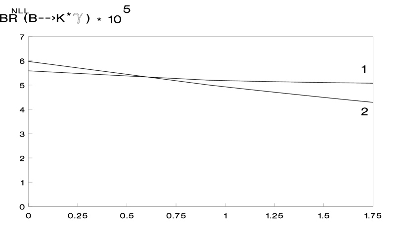
Figure 7: The branching ratio $Br(b\to K^{*}\gamma/10^{-5}$ as a function of $\log[1/\Lambda(GeV)]$ for the two methods discussed and $f_{B}$=160MeV.

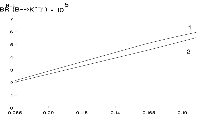
Figure 8: The branching ratio $Br(b\to K^{*}\gamma/10^{-5}$ as a function of $f_{B}$ for the two methods and $\Lambda=0.2GeV$

Our numerical results for the $B\to K^{*}\gamma$ decay rate are given in Table 1 in LL and NLL approximation (for the two methods to regularize the IR divergences). The dependence on the cutoff $\Lambda$ is shown in Fig. 7, while the variation with $f_{B}$ is given in Fig. 8. For $f_{B}=160MeV$ and $\Lambda$=0.5GeV our prediction for the branching ratio is $(5.18\pm 0.5)\cdot 10^{-5}$ (method 1) and $(5.16\pm 0.5)\cdot 10^{-5}$ (method 2) (the errors refer to the scale uncertainty). For both methods, they are in agreement with the experimental value $BR(B\to K^{*}\gamma)=(4.2\pm 0.8\pm 0.6)\times 10^{-5}$ [2, 23], although it is somewhat on the high side. We note that with the simple expression for the vector meson wave function $\phi_{V}(y)=6y(1-y)$, the prediction for the branching is lowered by $\sim 15\%$. The NLL contributions clearly reduce the scale dependence of the LL result. For the decay rate in LL approximation, the uncertainty due to the scale dependence is 27%. On the other hand, the NLL results vary between 4% and 11% for method 1 and between 4% and 21% for method 2 for $1GeV>\Lambda>0.2GeV$. This remaining scale dependence is larger than the one of the inclusive decay. However, the standard model yields indeed an ’unnaturally’ low scale dependence for $b\to s\gamma$ [25]. Therefore the variation with the scale seems reasonable to us.

The uncertainty due to the unknown value of $\Lambda$ is between 6% and 14% for method 1 and between 10% and 26% for method 2. The results for the two methods for $\mu=5GeV$ and $0.2GeV<\Lambda<1GeV$ differ no more than 14%. Thus in method 1, the theoretical uncertainty is quite small, in the vicinity of 20%. If this is a correct assessment, then it is clearly desirable to improve the experimental accuracy.

The rather strong $\Lambda$ dependence of method 2 is clearly a shortcoming of this work. It arises mainly from the logarithmic cutoff singularity of the gluonic corrections to the operator $O_{7}$. A clear improvement would be to take into account three body Fock states (with an extra gluon) whose matrix element could remove the $\Lambda$ divergence. This requires relations between two-and three-body wave-functions. In simple cases, such relations exist [26]. However, a realistic calculation is beyond the state-of-the art. Another source of $\Lambda$ dependence lies in the ”inclusive” contributions associated with the operators $O_{2}$ and $O_{8}$. To isolate it, one would need a two-loop calculation with a finite cutoff; this is beyond the scope of this paper. We note here only that the corrections to $F[O_{2}]$, $F[O_{8}]$ vanish as $\Lambda$ goes to zero. We hope to return to these issues elsewhere. But if the three-body wave function indeed removes the low $\Lambda$ singularity, then a relatively low value of $\Lambda$, say $0.5$ GeV, would reproduce best the correct value of the branching ratio.

In conclusion, we have calculated the next-to-leading logarithmic corrections to the branching ratio of the exclusive $B\to K^{*}\gamma$ decay, using an “inclusive” method and an IR cutoff parameter $\Lambda$ to remove possible infrared divergences. For $f_{B}=160MeV$ and $\Lambda$=0.5 GeV, the prediction for the branching ratio is $(5.18\pm 0.5)\cdot 10^{-5}$ and $(5.16\pm 0.5)\cdot 10^{-5}$ for two IR regularization methods we use. This corresponds to a 10% increase over the leading order calculation. The $\Lambda$ dependence is sizeable, around 20%. We discuss possible ways to improve this uncertainty.

Acknowledgments

We thank Ch. Greub, S. Brodsky, A. Khodjamirian and R. Poghosian for discussions. This work was partially supported by INTAS under Contract INTAS-96-155 and by the Swiss Science Foundation.

APPENDIX A

In this Appendix we present the results for the matrix element of inclusive $b\to s\gamma$ decay associated with the operator $O_{7}$ when we use a cutoff (method 2). The corresponding diagrams for the wave function renormalization factors $Z_{2}^{(b)}$ and $Z_{2}^{(s)}$ and the vertex operator are shown in Fig. 2. Following [8], we introduce the renormalization scale in the form $\mu^{2}\exp(\gamma_{E})/(4\pi)$. Then the $\overline{MS}$ subtraction corresponds to subtracting poles in $\epsilon$ in the dimensional regularization scheme.

First we present the results for nonzero gluon mass and without cutoff. For that case $Z_{2}^{(b)}$ is given by:

$$\Sigma^{(b)}=\frac{1}{i}\frac{\alpha_{s}}{3\pi^{3}}(2\pi)^{2\epsilon}\left(\frac{\mu^{2}}{4\pi}\right)^{\epsilon}\exp(\epsilon\gamma_{E})\int_{-\infty}^{\infty}d^{d}q\int_{0}^{1}dx\frac{4m_{b}-2(\hat{p^{{}^{\prime}}}-\hat{q})}{(q^{2}-2xp^{{}^{\prime}}\cdot q-r^{2})^{2}}$$

$$(Z_{2}^{(b)})^{-1}-1=-\frac{d\Sigma^{(b)}}{d\hat{p^{{}^{\prime}}}}_{\hat{p^{{}^{\prime}}}=m_{b}},$$ (A.1)

where $\mu_{0}$ is the gluon mass, $r^{2}=xm_{b}^{2}+(1-x)\mu_{0}^{2}-xp^{{}^{\prime}2}$. Then the integral over q is performed and we obtain:

$$Z_{2}^{(b)}=1+\frac{\alpha_{s}}{3\pi}\left(1+\int_{0}^{1}dx\left(-4(1-x)\log\frac{\mu^{2}}{\Delta_{b}}+8x(1-x^{2})\frac{m_{b}^{2}}{\Delta_{b}}\right)\right)$$

$$\Delta_{b}=x^{2}m_{b}^{2}+(1-x)\mu_{0}^{2}$$ (A.2)

The expression for $Z_{2}^{(s)}$ can be obtained from (A.2) via the substitution $m_{b}\to m_{s}$. The contribution of the vertex diagram Fig 2b is given by

$$V=\frac{2\alpha_{s}}{3i\pi^{3}}\frac{em_{b}}{8\pi^{2}}\int d^{4}q\int_{0}^{1}dx_{1}\int_{0}^{x_{1}}dx_{2}\frac{4\hat{\epsilon}\hat{k}R(p_{b}\cdot p_{s})-2(\hat{\epsilon}\hat{k}R\hat{q}\hat{p_{s}}+\hat{p_{b}}\hat{q}\hat{\epsilon}\hat{k}R)}{(q^{2}-2(p\cdot q)-t^{2})^{3}}$$ (A.3)

where $p=(x_{1}-x_{2})p_{b}+(1-x_{1})p_{s}$, $t^{2}=(x_{1}-x_{2})(m_{b}^{2}-p_{b}^{2})+(1-x_{1})(m_{s}^{2}-p_{s}^{2})+x_{2}\mu_{0}^{2}$. After integrating over q, V can be expressed in the following form:

$$V=<s\gamma|O_{7}|b>_{tree}V_{1}$$ (A.4)

$$V_{1}=-\frac{2\alpha_{s}}{3\pi}\int_{0}^{1}dx_{1}\int_{0}^{x_{1}}dx_{2}\frac{x_{2}(m_{b}^{2}+m_{s}^{2})}{x_{2}\mu_{0}^{2}+(1-x_{2})((x_{1}-x_{2})m_{b}^{2}+(1-x_{1})m_{s}^{2})}.$$

Finally, the contribution of $O_{7}$ for the case of nonzero gluon mass is given by

$$<s\gamma|O_{7}|b>_{\mu_{0}}=<s\gamma|O_{7}|b>_{tree}\left(1+V_{1}+\frac{8\alpha_{s}}{4\pi}\log\frac{m_{b}}{\mu}+\left(\sqrt{Z_{2}^{(b)}Z_{2}^{(s)}}-1\right)\right).$$ (A.5)

Now we proceed to the case when we introduce a cutoff parameter $\Lambda$. We calculate the integrals for the region $|q^{2}|<\Lambda^{2}$ and use then the previous results to obtain the integrals over the region $|q^{2}|>\Lambda^{2}$. We have the following expressions:

$$\Sigma_{\Lambda}^{(b)}=\frac{1}{i}\frac{\alpha_{s}}{3\pi^{3}}(2\pi)^{2\epsilon}\left(\frac{\mu^{2}}{4\pi}\right)^{\epsilon}\exp(\epsilon\gamma_{E})\int_{|q^{2}|<\Lambda^{2}}d^{d}q\int_{0}^{1}dx\frac{4m_{b}-2(\hat{p^{{}^{\prime}}}-\hat{q})}{(q^{2}-2x(p^{{}^{\prime}}\cdot q)-r^{2})^{2}}$$

$$\frac{1}{(Z_{2}^{(b)})_{|q^{2}|<\Lambda^{2}}}-1=-\frac{d\Sigma^{(b)}_{\Lambda}}{d\hat{p^{{}^{\prime}}}}_{\hat{p^{{}^{\prime}}}=m_{b}},$$ (A.6)

$$V_{|q^{2}|<\Lambda^{2}}=\frac{2\alpha_{s}}{3i\pi^{3}}\frac{em_{b}}{8\pi^{2}}\int_{|q^{2}|<\Lambda^{2}}d^{4}q\int_{0}^{1}dx_{1}\int_{0}^{x_{1}}dx_{2}\frac{4\hat{\epsilon}\hat{k}R(p_{b}\cdot p_{s})-2(\hat{\epsilon}\hat{k}R\hat{q}\hat{p_{s}}+\hat{p_{b}}\hat{q}\hat{\epsilon}\hat{k}R)}{(q^{2}-2(p\cdot q)-t^{2})^{3}}$$ (A.7)

We have the following integrals:

$$\Sigma_{2\Lambda}^{(b1)}=\frac{2}{3\pi^{3}}\int_{|q^{2}|<\Lambda^{2}}d^{4}q\frac{1}{(q^{2}-2x(p^{{}^{\prime}}\cdot q)-r^{2})^{2}}$$

(A.8)

$$\Sigma_{2\Lambda}^{(b2)}=\frac{2}{3\pi^{3}}\int_{|q^{2}|<\Lambda^{2}}d^{4}q\frac{q\cdot p^{{}^{\prime}}}{p^{{}^{\prime}2}(q^{2}-2x(p^{{}^{\prime}}\cdot q)-r^{2})^{2}}$$

$$V_{\Lambda}^{(1)}=\frac{4}{3\pi^{3}}\int_{|q^{2}|<\Lambda^{2}}d^{4}q\frac{1}{(q^{2}-2(p\cdot q)-t^{2})^{3}}$$

(A.9)

$$V_{\Lambda}^{(2)}=\frac{4}{3\pi^{3}}\int_{|q^{2}|<\Lambda^{2}}d^{4}q\frac{q\cdot p}{p^{2}(q^{2}-2(p\cdot q)-t^{2})^{3}}$$

The integrals over the momentum q are performed using a Wick rotation and we obtain:

$$\Sigma_{2\Lambda}^{(b1)}=\frac{1}{6\pi x^{2}p^{{}^{\prime}2}}\left\{\Lambda^{2}+r^{2}-\sqrt{\Lambda^{4}+r^{4}+2\Lambda^{2}(r^{2}+2x^{2}p^{{}^{\prime}2})}-\right.$$

$$\left.-2x^{2}p^{{}^{\prime}2}\left[{\rm arctanh}\left(1+\frac{2x^{2}p^{{}^{\prime}2}}{r^{2}}\right)+{\rm arctanh}\left(\frac{-2x^{2}p^{{}^{\prime}2}-r^{2}-\Lambda^{2}}{\sqrt{\Lambda^{4}+r^{4}+2\Lambda^{2}(r^{2}+2x^{2}p^{{}^{\prime}2}}}\right)\right]\right\}$$

$$\Sigma_{2\Lambda}^{(b2)}=-\frac{1}{12\pi x^{3}}\left\{\frac{1}{p^{{}^{\prime}4}}\left(\Lambda^{4}+r^{2}(r^{2}-2x^{2}p^{{}^{\prime}2})-(\Lambda^{2}+r^{2}-2x^{2}p^{{}^{\prime}2})\sqrt{\Lambda^{4}+r^{4}+2\Lambda^{2}(r^{2}+2x^{2}p^{{}^{\prime}2})}+\right.\right.$$

$$\left.\left.+2r^{2}\Lambda^{2}\right)+4x^{4}\left[{\rm arctanh}\left(1+\frac{2x^{2}p^{{}^{\prime}2}}{r^{2}}\right)+{\rm arctanh}\left(\frac{-2x^{2}p^{{}^{\prime}2}-r^{2}-\Lambda^{2}}{\sqrt{\Lambda^{4}+r^{4}+2\Lambda^{2}(r^{2}+2x^{2}p^{{}^{\prime}2}}}\right)\right]\right\}$$

$$V_{\Lambda}^{(1)}=\frac{(-\Lambda^{2}(2p^{2}+t^{2})-t^{4})\sqrt{(\Lambda^{2}+t^{2})^{2}+4p^{2}\Lambda^{2}}+t^{2}((\Lambda^{4}+t^{4}+\Lambda^{2}(4p^{2}+2t^{2}))}{3\pi p^{2}(p^{2}+t^{2})((\Lambda^{2}+t^{2})^{2}+4p^{2}\Lambda^{2})}$$ (A.10)

$$V_{\Lambda}^{(2)}=-\frac{(\Lambda^{2}(p^{2}+t^{2})+t^{4})\sqrt{(\Lambda^{2}+t^{2})^{2}+4p^{2}\Lambda^{2}}-\Lambda^{4}(p^{2}+t^{2})-t^{2}\Lambda^{2}(3p^{2}+2t^{2})-t^{6}}{3\pi p^{4}(p^{2}+t^{2})\sqrt{(\Lambda^{2}+t^{2})^{2}+4p^{2}\Lambda^{2}}}$$

where we take $t^{2}=x_{2}\mu_{0}^{2}$, $p^{2}=(1-x_{2})((x_{1}-x_{2})m_{b}^{2}+(1-x_{1})m_{s}^{2})$, $r^{2}=(1-x)\mu_{0}^{2}$. Then $(Z_{2}^{(b)})_{|q^{2}|<\Lambda^{2}}$ and $V_{|q^{2}|<\Lambda^{2}}$ are equal to ($p^{{}^{\prime\prime}}=\sqrt{p^{{}^{\prime}2}}$)

$$V_{|q^{2}|<\Lambda^{2}}=<s\gamma|O_{7}|b>_{tree}\alpha_{s}\int_{0}^{1}dx_{1}\int_{0}^{x_{1}}dx_{2}(m_{b}^{2}+m_{s}^{2})\left(V_{\Lambda}^{(1)}-(1-x_{2})V_{\Lambda}^{(2)}\right)$$

$$(Z_{2}^{(b)})_{|q^{2}|<\Lambda^{2}}=1+\alpha_{s}\int_{0}^{1}dx\left(\frac{d}{d\hat{p^{{}^{\prime}}}}\left((4m_{b}-2\hat{p^{{}^{\prime}}})\Sigma_{2\Lambda}^{(b1)}+2\hat{p^{{}^{\prime}}}\Sigma_{2\Lambda}^{(b2)}\right)\right)_{\hat{p^{{}^{\prime}}}=m_{b}}=$$ (A.11)

$$=1+\alpha_{s}\int_{0}^{1}dx\left(2m_{b}\frac{d}{dp^{{}^{\prime\prime}}}\Sigma_{2\Lambda}^{(b1)}-2\Sigma_{2\Lambda}^{(b1)}+2m_{b}\frac{d}{dp^{{}^{\prime\prime}}}\Sigma_{2\Lambda}^{(b2)}+2\Sigma_{2\Lambda}^{(b2)}\right)$$

Then the expression for $(Z_{2}^{(b)})_{|q^{2}|>\Lambda^{2}}$ is given by the difference between $Z_{2}^{(b)}$ and $(Z_{2}^{(b)})_{|q^{2}|<\Lambda^{2}}$ while $V_{|q^{2}|>\Lambda^{2}}$ is given by the difference of V and $V_{|q^{2}|<\Lambda^{2}}$. For both cases, we can set the gluon mass equal to zero, i.e we take the limit $\mu_{0}\to 0$.

Figure Captions

Figure 1: Leading order contribution, associated with operator $O_{7}$.

Figure 2: Order $\alpha_{s}$ corrections for the b and s quark wave function renormalization and the operator $O_{7}$.

Figure 3: Order $\alpha_{s}$ corrections to the matrix element of the operator $O_{7}$ with gluon exchange between the quark lines.

Figure 4: Order $\alpha_{s}$ corrections to the matrix element of $O_{2}$ with gluon exchange between the quark lines and photon emission from external (a) and internal (b) quark lines. The crosses indicate the possible places of photon emission.

Figure 5: Order $\alpha_{s}$ corrections for the operator $O_{8}$ with gluon exchange. The possible places of photon emission are labelled with a cross.

Figure 6: The contributions of the operators $O_{i}$, i=1,2,3,4,5,6 with quark exchange. The possible places of photon emission are labelled with a cross.

	$\mu=2.5GeV$	$\mu=5GeV$	$\mu=10GeV$
$Br^{LL}(B\to K^{*}\gamma)/10^{-5}$	5.91	4.65	3.70
$Br^{NLL}(B\to K^{*}\gamma)/10^{-5}$, Method 1,$\Lambda$ =1GeV	5.35	5.59	5.48
$Br^{NLL}(B\to K^{*}\gamma)/10^{-5}$, Method 1, $\Lambda$ =0.5GeV	4.70	5.18	5.21
$Br^{NLL}(B\to K^{*}\gamma)/10^{-5}$, Method 1, $\Lambda$ =0.2GeV	4.55	5.09	5.16
$Br^{NLL}(B\to K^{*}\gamma)/10^{-5}$, Method 2, $\Lambda$ =1GeV	6.21	5.97	5.74
$Br^{NLL}(B\to K^{*}\gamma)/10^{-5}$, Method 2 $\Lambda$ =0.5GeV	4.66	5.16	5.20
$Br^{NLL}(B\to K^{*}\gamma)/10^{-5}$, Method 2, $\Lambda$ =0.2GeV	3.46	4.40	4.69

     

Figure 1: Leading order contribution, associated with operator $O_{7}$.

     

Figure 2: Order $\alpha_{s}$ corrections for the b and s quark wave function renormalization and the operator $O_{7}$.

     

Figure 3: Order $\alpha_{s}$ corrections to the matrix element of the operator $O_{7}$ with gluon exchange between the quark lines.

     

Figure 4: Order $\alpha_{s}$ corrections to the matrix element of $O_{2}$ with gluon exchange between the quark lines and photon emission from external (a) and internal (b) quark lines. The crosses indicate the possible places of photon emission.

     

Figure 5: Order $\alpha_{s}$ corrections for the operator $O_{8}$ with gluon exchange. The possible places of photon emission are labelled with a cross.

     

Figure 6: The contributions of the operators $O_{i}$, i=1,2,3,4,5,6 with quark exchange. The possible places of photon emission are labelled with a cross.

     

Figure 7: The branching ratio $Br(b\to K^{*}\gamma/10^{-5}$ as a function of $\log[1/\Lambda(GeV)]$ for the two methods discussed and $f_{B}$=160MeV.

     

Figure 8: The branching ratio $Br(b\to K^{*}\gamma/10^{-5}$ as a function of $f_{B}$ for the two methods and $\Lambda=0.2GeV$.

References

• [1] J. Hewett et al., in “The BABAR physics book”, SLAC-Report-504, October, 1998. M. Neubert, Talk given at ICHEP98, Vancouver, Canada 1998, Hep-ph/9809343.
• [2] R.Ammar et al. (CLEO Collaboration), Phys. Rev. Lett. 71 (1993) 674.
• [3] B. Grinstein, R. Springer and M. B. Wise, Nucl. Phys. B339 (1990).
• [4] A. J. Buras, M. Misiak, M. Münz and S. Pokorski, Nucl. Phys. B424 (1994) 374.
• [5] K. Adel, Y. P. Yao, Phys. Rev. D49 (1994) 495.
• [6] C. Greub, T. Hurth, Phys. Rev. D56 (1997) 2934.
• [7] A. Ali, C. Greub, Phys. Lett. B361 (1995) 146.
• [8] C. Greub, T. Hurth, D. Wyler, Phys. Rev. D54 (1996) 3350.
• [9] K. Chetyrkin, M. Misiak, M. Münz, Phys.Lett.B200 (1997) 206.
• [10] A. J. Buras, A Kwiatkowski and N Pott, Phys. Lett. B414 (1997) 157.
• [11] M. Ciuchini, G. Degrassi, P. Gambino and G. F. Giudice, Preprint CERN-TH-97279 (hep-ph/9710335).
• [12] M. S. Alam et al. (CLEO Collaboration), Phys. Rev. Lett. 74 (1995) 2885.
• [13] Z. Ligeti, M. B. Wise, Preprint FERMILAB-Pub-99/142-T. CALT-68-2224, hep-ph/9905277.
• [14] C. Greub, H. Simma, D. Wyler, Nucl.Phys. B434 (1995) 39.
• [15] A. Ali, H. Asatrian, C. Greub, Phys. Lett. B429 (1998) 87.
• [16] A. Buras, preprint TUM-HEP-316-98, hep-ph/9806471.
• [17] C. Greub, D. Wyler, Phys. Lett. B295 (1992) 293.
• [18] T. Altomari, Phys. Rev. D37 (1988) 677;
N. Isgur and M. Wise, Phys. Rev. D42 (1990) 2388;
D. Wyler, Nucl.Phys. (Proc. Suppl.) 7A (1989) 358;
A. Ali, T. Ohl and T. Mannel, Phys. Lett B298 (1993) 195;
C.A. Dominguez, N. Paver and Riazuddin, Phys. Lett. B214 (1988) 459;
T.M. Aliev, A.A. Ovchinnikov and V.A. Slobodeniuk;
Phys. Lett. B237 (1990) 569;
S. Narison, Phys. Lett. B327 (1994) 354;
P. Colangelo, C.A. Dominguez, G. Narduli and N. Paver, Phys. Lett B317 (1994) 354;
P. Ball, preprint hep-ph/9308244 ( unpublished);
D.R. Burford et al. (UKQCD Collab.), Nucl. Phys. B447 (1995) 425.
• [19] A. Ali, V. Braun, H . Simma, Z.Phys C63 (1994) 437.
• [20] G. Eilam, A. Ioannissian, R. R. Mendel, Z.Phys. C71 (1996) 95.
• [21] C. Caso et al., The European Physical Journal C3 (1998) 1.
• [22] S J. Brodsky, Preprint SLAC-PUB-7861, Invited talk at Workshop on Future Directions in Quark Nuclear Physics, Adelaide, Australia, 9-20 March 1998, hep-ph/9806445;
S J. Brodsky, Patrick Huet, Phys. Lett. B417 (1998) 145.
• [23] T. Skwarnicki, Preprint HEPSY 97-03, hep-ph/9712253.
• [24] S. Aoki et. al., Nucl.Phys.B Proc.Suppl. 60A (1998) 89, hep-lat/9711043.
• [25] M. Neubert, hep-ph/9809377. To be published in the proceedings ICHEP 98, Vancouver, Canada, 1998.
• [26] F. Antonuccio, S.J. Brodsky and S. Dalley (CERN), Phys.Lett.B 412 (1997) 104, hep-ph/9705413.