Generalized Sum Rules for Spin-Dependent
Structure Functions of the Nucleon

Abstract

The Drell-Hearn-Gerasimov and Bjorken sum rules are special examples of dispersive sum rules for the spin-dependent structure function $G_{1}(\nu,Q^{2})$ at $Q^{2}=0$ and $\infty$. We generalize these sum rules through studying the virtual-photon Compton amplitudes $S_{1}(\nu,Q^{2})$ and $S_{2}(\nu,Q^{2})$. At small $Q^{2}$, we calculate the Compton amplitudes at leading-order in chiral perturbation theory; the resulting sum rules can be tested by data soon available from Jefferson Lab. For $Q^{2}>\!\!>\Lambda_{\rm QCD}^{2}$, the standard twist-expansion for the Compton amplitudes leads to the well-known deep-inelastic sum rules. Although the situation is still relatively unclear in a small intermediate-$Q^{2}$ window, we argue that chiral perturbation theory and the twist-expansion alone already provide strong constraints on the $Q^{2}$-evolution of the $G_{1}(\nu,Q^{2})$ sum rule from $Q^{2}=0$ to $Q^{2}=\infty$.

I Introduction

In recent years, there has been great interest in studying the spin-dependent structure functions of the nucleon both in the deep-inelastic region and in the low-energy resonance region. These interests are spurred by a renewed effort to understand the internal spin structure of the nucleon and by experimental advances in polarized beam and target technology. The measurements of the structure functions $G_{1}(x,Q^{2})$ and $G_{2}(x,Q^{2})$ on proton, deuteron, and He³ targets in the deep-inelastic region by the EMC, SMC, E142, E143, E154, E155, and HERMES collaborations have provided rich information on the spin-dependent response of the nucleon for the first time [1]. New measurements from Jefferson Lab in Virginia and other low-energy facilities will provide additional information on these interesting physical observables [2].

A direct theoretical analysis of the nucleon structure functions is often difficult because they contain a sum over all nucleon final states. [An exception is the cut-vertex formalism developed by A. Mueller in the Bjorken region where the dominant excitations are few parton states [3].] Theoretical methods such as chiral perturbation theory [4] and the operator product expansion (OPE) [5] are more suitable for (virtual-) photon-nucleon Compton amplitudes. However, for a spacelike virtual photon there is no known way to measure the Compton amplitudes directly. Fortunately, the Compton amplitudes and the structure functions are related through dispersion relations. Hence theoretical predictions of Compton amplitudes can be tested against the measurable structure functions, provided the dispersion integrals converge.

The spin-dependent (virtual-) photon-nucleon Compton process can be described by the two Compton amplitudes $S_{1}(\nu,Q^{2})$ and $S_{2}(\nu,Q^{2})$, where $\nu$ and $Q^{2}$ are the virtual-photon energy and mass² in the target rest frame. The second amplitude decouples in the real photon ($Q^{2}=0$) limit. Many years ago, Low, Gell-Mann, and Goldberger showed that for a real photon the Compton amplitude $S_{1}(\nu,0)$ reduces to $-\kappa^{2}/M^{2}$ in the $\nu\rightarrow 0$ limit [6, 7], where $\kappa$ is the (dimensionless) anomalous magnetic moment of the nucleon. The result follows from electromagnetic gauge invariance and is nonperturbative in strong interaction physics. Using a dispersion relation for $S_{1}(\nu,Q^{2})$, Drell, Hearn, and Gerasimov (DHG) turned this theoretical prediction into a sum rule for the spin-dependent photonucleon production cross sections [8]

$$\int^{\infty}_{\nu_{\rm in}}{d\nu\over\nu}(\sigma_{P}(\nu)-\sigma_{A}(\nu))={2\pi^{2}\alpha_{\rm em}\kappa^{2}\over M^{2}},$$ (1)

where $\sigma_{P,A}(\nu)$ is the total photonucleon cross section with photon energy $\nu$. The labels $P$ and $A$ refer to whether the helicity of the photon is parallel or antiparallel to the spin of the nucleon, respectively. The integration begins at the inelastic threshold, denoted here by $\nu_{\rm in}$. We note that the spin-dependent photonucleon cross section is proportional to the $G_{1}$ structure function: $G_{1}(\nu,0)=-1/(8\pi^{2}\alpha_{\rm em})(\sigma_{P}(\nu)-\sigma_{A}(\nu))$.

In the opposite limit $Q^{2},\nu\rightarrow\infty$ while $Q^{2}/\nu$ remains finite, Bjorken derived a sum rule for the $G_{1}(\nu,Q^{2})$ structure function using the current algebra method [9]

$$\lim_{Q^{2}\rightarrow\infty}\int_{0}^{1}dx(g_{1}^{(p)}(x,Q^{2})-g_{1}^{(n)}(x,Q^{2}))={g_{A}\over 6},$$ (2)

where $g_{1}(Q^{2}/2M\nu,Q^{2})=M\nu G_{1}(\nu,Q^{2})$ is a dimensionless scaling function, $g_{A}$ is the neutron decay constant, and the superscripts on $g_{1}$ refer to the target nucleon (proton or neutron). The modern approach to deriving the Bjorken sum rule starts with the operator product expansion for the Compton amplitude $S_{1}(0,Q^{2})$. It is easy to show that as $Q^{2}\rightarrow\infty$

$$S_{1}^{(p)}(0,Q^{2})-S_{1}^{(n)}(0,Q^{2})={4\over 3Q^{2}}g_{A}\ .$$ (3)

This result can turned into Eq. (2) by a simple use of the dispersion relation for $S_{1}(\nu,Q^{2})$.

The actual test of the Bjorken sum rule is not made at $Q^{2}=\infty$, but at finite $Q^{2}$ (2 to 10 GeV²) [1]. This requires a generalization of the Bjorken prediction for $S_{1}(0,Q^{2})$ to finite $Q^{2}$. The OPE is again a natural tool for this. Near $\nu=0$, $S_{1}(\nu,Q^{2})$ and $S_{2}(\nu,Q^{2})$ can be expanded in Taylor series in $\nu$. The coefficient of $\nu^{n}$ can be calculated as a double expansion in $\alpha_{s}(Q^{2})$ (QCD perturbation theory) and $1/Q^{2}$ (the twist expansion). For sufficiently large $Q^{2}$ where the high-twist terms can be neglected, the generalization of the Bjorken sum rule involves calculations of well-defined perturbative diagrams [10].

In this paper, we are mainly concerned with the generalization of the Drell-Hearn-Gerasimov sum rule to non-zero $Q^{2}$. According to the above discussion, this requires a theoretical study of the $S_{1,2}(\nu,Q^{2})$ amplitudes in the low $Q^{2}$ and $\nu$ region. We use chiral perturbation theory because it is the natural tool in this kinematic regime [4]. We notice that many previous works have used virtual-photon cross sections instead of the $G_{1}(\nu,Q^{2})$ structure function to generalize the DHG integral [11]. We argue that these generalizations are neither unique nor theoretically appealing because no actual sum rule for the integral has been established in these works.

It is interesting to study the $Q^{2}$-evolution of $S_{1}(0,Q^{2})$ as it determines the $Q^{2}$ evolution of the $G_{1}(\nu,Q^{2})$ sum rule. We will argue that chiral perturbation theory (the hadron description) allows us to understand the $Q^{2}$-dependence from $Q^{2}=0$ to the neighborhood of 0.2 GeV² and the OPE (the parton description) from $Q^{2}=\infty$ to the neighborhood of 0.5 GeV². For the window between $Q^{2}=0.2$ to $0.5$ GeV², where Jefferson Lab will collect precise data [2], we do not yet have a firm theoretical understanding of $S_{1,2}(\nu,Q^{2})$. Therefore, it provides an interesting ground on which to test various theoretical ideas.

This paper is organized as follows. In Section II, we specify definitions and notations. More importantly, we will present the dispersion relations and discuss their convergence. In Section III, we consider the DHG sum rule and its perturbative implications, particularly in chiral perturbation theory. In Section IV, we calculate $S_{1}(0,Q^{2})$ to leading order in relativistic chiral perturbation theory and translate the result into a generalized DHG sum rule. We also discuss the phenomenological implications of the result. In section V, we consider a technical point— the use of heavy-baryon chiral perturbation theory in our calculations. In section VI, we present more general predictions for the $S_{1,2}(\nu,Q^{2})$ amplitudes and suggest ways to test these predictions. In Section VII, we focus on the $Q^{2}$-evolution of the the simplest $G_{1}(\nu,Q^{2})$ sum rule and emphasize the concept of parton-hadron duality. At the same time, we point out the role of the nucleon elastic contribution in the sum. Finally, we summarize our results in Section VIII.

II Dispersion Relations and Convergence

This section contains no new results. Rather, it introduces the various notations and definitions which will be useful in subsequent sections. Moreover, we state the main theoretical assumption which relates the (virtual-) photon Compton amplitudes to the nucleon structure functions: the dispersion relations. Although these relations are not as sacred as Lorentz symmetry or locality, they are derived based on the fairly general grounds. Therefore, the attitude we take in this paper is that they can be used to test theoretical predictions of the Compton amplitudes. However, to satisfy the purists, we will quote some standard arguments justifying the use of unsubtracted integrals.

In inclusive lepton-nucleon scattering through one-photon exchange, the cross section depends on the tensor [12]

$$W^{\mu\nu}={1\over 4\pi}\int d^{4}\xi e^{iq\cdot\xi}\langle PS|[J^{\mu}(\xi),J^{\nu}(0)]|PS\rangle,$$ (4)

where $|PS\rangle$ is the covariantly-normalized ground state of a nucleon with momentum $P^{\mu}$ and spin polarization $S^{\mu}$ and $J_{\mu}=\sum_{i}e_{i}\bar{\psi}_{i}\gamma_{\mu}\psi_{i}$ is the electromagnetic current (with $\psi_{i}$ the quark field of flavor $i$ and $e_{i}$ its charge in units of the proton charge). The four-vector $q^{\mu}$ is the virtual-photon four-momentum. Using Lorentz symmetry, time-reversal, and parity invariance, one can express the spin-dependent ($\mu\nu$ antisymmetric) part of $W$ as

$$W^{[\mu\nu]}(P,q,S)=-i\epsilon^{\mu\nu\alpha\beta}q_{\alpha}\left[S_{\beta}G_{1}(\nu,Q^{2})+(M\nu\,S_{\beta}-S\cdot q\,P_{\beta})G_{2}(\nu,Q^{2})\right]\ ,$$ (5)

where $\epsilon^{0123}=+1$ and $M$ is the nucleon mass. $G_{1,2}(\nu,Q^{2})$ are the two spin-dependent structure functions of the nucleon, which depend on two independent Lorentz scalar variables $Q^{2}=-q^{2}$ and $\nu=P\cdot q/M$. In the rest frame of the nucleon, $\nu$ is the photon energy. [Since $S^{\mu}$ is present only in the external nucleon states, it only appears in the Lorentz structure, not in the scalar structure functions.] At times, we use the Bjorken variable $x=Q^{2}/2M\nu$ to replace the variable $\nu$. For our purposes, we assume $G_{1,2}(\nu,Q^{2})$ are measurable in the whole kinematic region $0<Q^{2},\nu<\infty$.

A quantity closely-related to the hadron tensor is the forward virtual-photon Compton tensor,

$$T^{\mu\nu}=i\int d^{4}\xi e^{iq\cdot\xi}\langle PS|{\rm T}J^{\mu}(\xi)J^{\nu}(0)|PS\rangle\ ,$$ (6)

which differs from $W^{\mu\nu}$ by the time ordering. Because of this, standard Feynman perturbation theory can be used to calculate $T^{\mu\nu}$ directly. Its antisymmetric part can also be expressed in terms of two scalar functions:

$$T^{[\mu\nu]}(P,q,S)=-i\epsilon^{\mu\nu\alpha\beta}q_{\alpha}\left[S_{\beta}S_{1}(\nu,Q^{2})+\left(M\nu\,S_{\beta}-S\cdot q\,P_{\beta}\right)S_{2}(\nu,Q^{2})\right]\ .$$ (7)

We call $S_{1,2}(\nu,Q^{2})$ the spin-dependent Compton amplitudes.

The Compton amplitudes can be analytically continued to the complex-$\nu$ plane. They are real on the real axis near $\nu=0$. They have poles at $\nu=\pm Q^{2}/2M$, corresponding to $s$- and $u$-channel elastic scattering, and two cuts on the real axis entending from $\nu=\pm\nu_{\rm in}$ to $\nu=\pm\infty$. The $s$- and $u$-channel symmetry leads to the following crossing relations

$$S_{1}(\nu,Q^{2}) = S_{1}(-\nu,Q^{2})\ ,$$ (8)

$$S_{2}(\nu,Q^{2}) = -S_{2}(-\nu,Q^{2})\ .$$ (9)

The $G_{1,2}(\nu,Q^{2})$ structure functions are proportional to the imaginary parts of the Compton amplitudes on the real axis:

$${\rm Im}~{}S_{i}(\nu,Q^{2})=2\pi G_{i}(\nu,Q^{2})\ ,$$ (10)

where $\nu$ is approaching the positive real axis from above and the negative real axis from below.

Applying Cauchy’s theorem and assuming $S_{i}(\nu,Q^{2})$ vanishes sufficiently fast as $\nu\rightarrow\infty$, we can write down the dispersion relations [12]

$$S_{1}(\nu,Q^{2}) = 4\int^{\infty}_{Q^{2}/2M}{d\nu^{\prime}\nu^{\prime}G_{1}(\nu^{\prime},Q^{2})\over\nu^{\prime 2}-\nu^{2}}\ ,$$ (11)

$$S_{2}(\nu,Q^{2}) = 4\int^{\infty}_{Q^{2}/2M}{d\nu^{\prime}\nu G_{2}(\nu^{\prime},Q^{2})\over\nu^{\prime 2}-\nu^{2}}\ ,$$ (12)

where we have used the crossing symmetry. Using these relations, theoretical predictions of the Compton amplitudes can be translated into dispersive sum rules for the structure functions.

One question often raised about the dispersion relations is their convergence at high-energy. On quite general grounds, one would argue that the above integrals converge. Considering the real photon case, for instance, it is reasonable to expect the photoproduction cross sections to be spin-independent at high energy.

The standard practice is to resort to Regge phenomenology, which has actually never been tested thoroughly in spin-dependent and/or virtual photon scattering cases. According to the folklore, $G_{1}(\nu,Q^{2})$ in the isovector channel behaves as $\nu^{\alpha_{a_{1}}(0)-1}$ at large $\nu$, where $\alpha_{a_{1}}(0)$ is the Regge intercept of the $a_{1}$ trajectory at $t=0$ (forward scattering). Since $\alpha_{a_{1}}(0)$ is believed to be somewhere between $-0.5$ and $0$, the convergence of the integral is guaranteed. However, in the isoscalar channel the picture is not so clear. Most of the studies so far favor a convergent integral [13]. When the integrals do converge, there is still the insidious possibility that they do not converge to the Compton amplitudes [12]. Such a possibility is quite remote in QCD given the accuracy of the experimental tests of the Bjorken sum rule [1]. As for the $G_{2}(\nu,Q^{2})$ integral, convergence apparently happens for any reasonable Regge behavior [14].

Of course, independent of the theoretical guesses, study of the high-energy behavior of the spin-dependent structure functions should be an important part of future experimental programs. However, in the remainder of the paper, we take it as a good working hypothesis that the above dispersion relations are valid without subtraction.

III The Drell-Hearn-Gerasimov Sum Rule And Chiral Perturbation Theory

As we have explained above, the DHG sum rule depends on two theoretical statements : the low-energy theorem for the spin-dependent amplitudes [6, 7] and unsubtracted dispersion relation for the relevant Compton amplitude. Although both are of a nonperturbative nature, it is interesting to consider them in the context of perturbation theory. In particular, since we are interested in the DHG sum rule for the nucleon, we would like to consider carefully its significance in chiral perturbation theory.

The low-energy theorem is related to electromagnetic gauge invariance [6, 7, 15]. It is a nonperturbative result which is independent of the detailed dynamics of the bound state under consideration. Using the notation introduced above, the low-energy theorem states that for a spin-1/2 target

$$S_{1}(\nu,0)\rightarrow-{\kappa^{2}\over M^{2}}\$$ (13)

as $\nu\rightarrow 0$, where $\kappa$ is the anomalous magnetic moment of the object under consideration.

The above result has interesting implications on the power series for $S_{1}(0,0)$ if the structure of the target can be understood in perturbation theory. Consider, for instance, $S_{1}(0,0)$ for the electron in quantum electrodynamics. Since $\kappa_{\rm e}=\alpha_{\rm em}/2\pi+...$, the leading contribution to $S_{1}(0,0)$ must be of order $\alpha_{\rm em}^{2}$. This means that all contributions to $S_{1}(0,0)$ of order $\alpha_{\rm em}$ must add up to zero. Indeed, if one computes $S_{1}(0,0)$ explicitly from the four diagrams shown in Fig. 1, one finds that all contributions add up to zero. At the next order, one has many more diagrams. The sum of all the diagrams must add up to the square of Schwinger’s result.

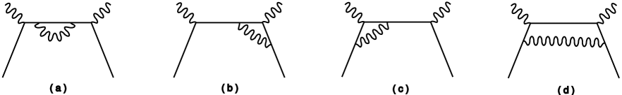
FIG. 1.: Photon-electron Compton scattering at one-loop order.

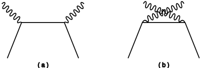
FIG. 2.: Nucleon pole diagrams for photon-nucleon Compton scattering.

Now we turn to chiral perturbation theory for the low energy structure of the nucleon. At leading order, the nucleon couples to photons through the following effect vertex,

$$\Gamma^{\mu}=e\gamma^{\mu}+i\kappa_{0}{\sigma^{\mu\nu}q_{\nu}\over 2M},$$ (14)

where $\kappa_{0}$ is the anomalous magnetic moment of the nucleon in the chiral limit. The nucleon-pole diagrams (shown in Fig. 2) yield the following contribution to $S_{1}(0,0)$ :

$$S_{1}(0,0)^{N-{\rm pole}}=-{\kappa_{0}^{2}\over M^{2}}.$$ (15)

Comparing this with the low-energy theorem, one concludes that the leading chiral contributions to $S_{1}(0,0)$ must sum to zero.

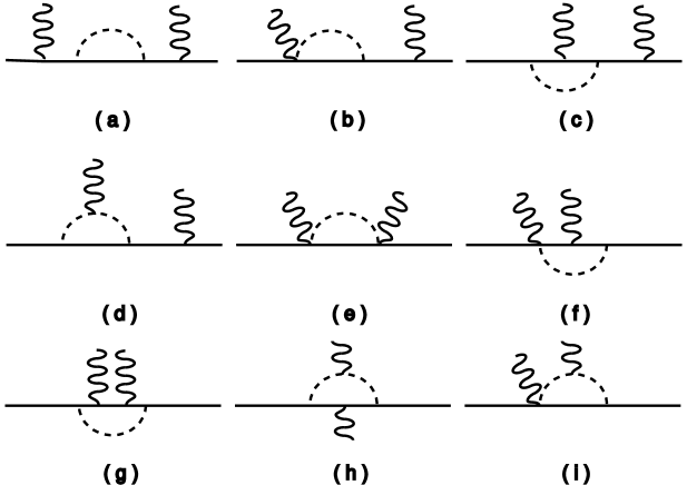
FIG. 3.: Photon-nucleon Compton diagrams at one-loop order in chiral perturbation theory.

We consider the one-loop contributions $S_{1}(0,0)$ in chiral perturbation theory shown in Fig. 3. There are nine topologically distinct diagrams. All others can be obtained by switching the initial and final state nucleon or by exchanging the photons (crossing symmetry). All of these diagrams contribute to $S_{1}(0,0)$, as shown in Table 1.

Diagram	Isospin Factor	Constant	$\log(m_{\pi}^{2}/m^{2})$	$2/\epsilon-\log(m^{2}/4\pi\mu^{2})$
3a	$1/2+t_{3}$	$9/4$	0	$3/4$
3b	$1/2+t_{3}$	$-1$	0	$-1$
3c	$1/2+t_{3}$	0	0	$-1/2$
3d	$1/2+t_{3}$	1	1	0
3e	1	$3/2$	0	$1/2$
3f	$1/2-t_{3}$	2	0	$-1$
3g	$3/2-t_{3}$	$-3/4$	0	$1/4$
3h	$1/2-t_{3}$	1	1	0
3i	1	$-3$	$-1$	0

TABLE I.: Contributions to $S_{1}(0,0)$ from the diagrams in Fig. 3. All contributions have the common factor $2(g_{A}/4\pi f_{\pi})^{2}$. We note that although the sum of each column is indeed zero, the cancellation is highly nontrivial.

We note that all diagrams without the attachment of a photon to the pion loop are ultraviolet divergent. However, all divergences cancel out. The sum of all contributions is indeed zero, as required by gauge-invariance.

When combining the low-energy theorem with the unsubtracted dispersion relation, one obtains the DHG sum rule. If one has a fundamental theory in which particles are pointlike, the DHG sum rule is correct order by order, and even diagram by diagram, in perturbation theory. In QED and the standard model of electroweak interactions, this result has been shown at leading order in perturbation theory [16]. Recently, Brodsky and Schmidt have generalized Altarelli et al.’s result for any $2\rightarrow 2$ process to supersymmetric and other quantum field theories [17].

However, it must pointed out that in an effective theory where the particles have internal structure, the DHG sum rule cannot be correct order by order in perturbation theory. Indeed, recall the $s$-channel nucleon-pole diagram which contributes to $S_{1}(0,0)$. This digram does not have an imaginary part because elastic scattering is forbidden in this case by kinematics (unless $\nu$ is strictly zero). However, it gives the entire low-energy-theorem result in the chiral limit. The unsubtracted dispersion relation clearly does not work for this diagram. An opposite example is the diagram with a $\Delta$ pole. We will see in Sec. VI that this diagram does not contribute to $S_{1}(0,0)$, but it completely dominates the DHG integral in the limit of a large number of color [18]. Again, we see that an unsubtracted dispersion relation fails for the diagram. In general, since the effective theory is only good at low-energy, it cannot be used to calculate the photon absorption cross section at very high-energy, and hence one cannot establish any dispersion relation between the real and imaginary parts of the Compton amplitudes in the theory.

It is interesting to note here that a perturbative verification of the DHG sum rule in the context of quantum gravity can have implications about physics beyond the string compatification scale [19].

IV Generalized Drell-Hearn-Gerasimov Sum Rule

As we have discussed above, the Drell-Hearn-Gerasimov sum rule has its origin in the dispersion relation and the low-energy theorem for the Compton amplitude $S_{1}(0,0)$. To extend the sum rule to virtual-photon scattering, we take $\nu=0$ in Eq. (12)

$$S_{1}(0,Q^{2})=4\int^{\infty}_{Q^{2}/2M}{d\nu\over\nu}G_{1}(\nu,Q^{2})\ .$$ (16)

This would be a general $Q^{2}$-dependent sum rule provided one knew how to extend the theoretical prediction for the Compton amplitude $S_{1}(0,Q^{2})$ beyond the low-energy theorem.

We notice that the popular way to generalize the DHG sum rule in the literature has been to consider an integration over the spin-dependent virtual-photon-nucleon cross section (referred to as the DHG integral) [11]. Indeed, in some experimental publications, the data has been presented in this way [20]. [The model calculation presented in Ref. [21] is an exception.] The problem we have with this is that the virtual-photon cross section is not a well-defined quantity because the virtual-photon flux is convention-dependent. More importantly, in these types of proposals, no rule has been specified as to what the DHG integral should be equal to. If one does not have a rule for the sum, there is no point to study the sum. One can just as well study the individual contributions. The generalized DHG sum rule implied in Eq. (16) is not only Lorentz-invariant, but also exhibits clear physical significance: The integral gives rise to the virtual-photon Compton amplitude $S_{1}(0,Q^{2})$.

If $Q^{2}$ is very small compared with the nucleon mass, $S_{1}(0,Q^{2})$ should be computable in chiral perturbation theory. In recent years, chiral perturbation theory ($\chi$PT) has emerged as a powerful tool to go beyond the various low-energy theorems involving pions, photons, and nucleons [4, 22]. In this and the next two sections, we study the implications of $\chi$PT for the $S_{1,2}(\nu,Q^{2})$. We notice that a study of a generalized DHG sum rule via a dispersion relation in $\chi$PT has in fact been made in Ref. [23]. However, our view on the subject is significantly different and we will point out the differences towards the end of this section.

In this section, we are interested in the leading-order chiral perturbation theory prediction for $S_{1}(0,Q^{2})$. Let us make an important point first. As soon as $Q^{2}\neq 0$, the Compton amplitude receives an a contribution from elastic scattering. This contribution can be calculated simply in terms of the Dirac and Pauli form factors of the nucleon

$$S_{1}^{\rm el}(0,Q^{2})={4\over Q^{2}}F_{1}(Q^{2})(F_{1}(Q^{2})+F_{2}(Q^{2}))\ .$$ (17)

This elastic contribution dominates at low $Q^{2}$ due to the $1/Q^{2}$ singularity. Since the DHG sum rule has no elastic contribution due to the kinematic constraint, we consider a subtracted version of $S_{1}$

$$\overline{S}_{1}(0,Q^{2})=S_{1}(0,Q^{2})-S_{1}^{\rm el}(0,Q^{2})\ ,$$ (18)

which then can be expanded around $Q^{2}=0$:

$${\overline{S}_{1}}(0,Q^{2})=-{\kappa^{2}\over M^{2}}+{\overline{S}_{1}}^{\prime}(0,0)Q^{2}+{1\over 2}{\overline{S}_{1}}^{\prime\prime}(0,0)Q^{4}+...\ .$$ (19)

In $\chi$PT, the coefficient ${\overline{S}_{1}}^{\prime}(0,0)$ can be expanded as a power series in pion mass:

$${\overline{S}_{1}}^{\prime}(0,0)={a\over m_{\pi}^{2}}+{b\over m_{\pi}}(\log m_{\pi}+\beta)+...\ .$$ (20)

The leading chiral contribution comes from the $a$ term.

We will calculate $a$ using heavy-baryon chiral perturbation theory (HB$\chi$PT) in which one formally takes the nucleon mass to infinity [24]. HB$\chi$PT is entirely equivalent to $\chi$PT using the fully relativistic propagators except that the former has a better way to organize different powers of the nucleon mass. There is, however, a subtle point in calculating $S_{1}(0,Q^{2})$ due to the special kinematics. We will discuss this point in the next section.

The leading chiral contribution comes from diagrams in which one of the two photons lands on a pion. This physically makes sense because in the chiral limit, the nucleon has a pion cloud extending far away from it and the leading scattering process is one in which the photon directly interacts with the pion. At one-loop order, only diagrams $d,h,$ and $i$ of Fig. 3 contribute. However, when we add their contributions together, we get

$$a=0\ .$$ (21)

In other words, the leading chiral contribution vanishes. To understand this, we recall that in the heavy-baryon limit spin-dependent effects vanish like $1/M$. This physical fact gives rise to the well-known heavy-quark symmetry in heavy-quark physics [25]. In the present case, the symmetry implies that the leading chiral terms $(Q^{2})^{n}/m_{\pi}^{2n}$ vanish in Eq. (19). Our calculation confirms this.

The above result has interesting phenomenological implications. At present, there is no direct data on the spin-dependent photo-production cross section, and therefore one cannot make a direct test of the DGH sum rule. However, there is already data available for ${G_{1}}(\nu,Q^{2})$ at low $Q^{2}$. The lowest $Q^{2}$ of the data is around $m_{\pi}^{2}\sim 0.02$ GeV². At this point ${\overline{S}_{1}}(0,Q^{2})$ differs from ${\overline{S}_{1}}(0,0)=-\kappa^{2}/M^{2}$ by a quantity of order ${Q^{2}/m_{\pi}M^{3}}\sim(m_{\pi}/M)/M^{2}=0.15/M^{2}$. Baring an anomalously large coefficient, the correction is of only a few percent!

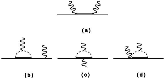
FIG. 4.: Photon-nucleon Compton diagrams with the $\Delta$ as an intermediate state.

What about contributions from the $\Delta$-resonance, whose mass is about $2m_{\pi}$ larger than the nucleon mass? In the large $N_{c}$ limit, the $\Delta$ is degenerate with the nucleon and clearly plays a very important role. Thus, we need to get an idea how important the $\Delta$ is in the real world. First of all, direct $\Delta$ production, shown in Fig. 4a, gives a contribution of zero. This is somewhat surprising given the fact that the $\Delta$ contributes dominantly on the dispersive side of the DHG sum rule. However, as we have mentioned before, one cannot establish a dispersion relation in an effective theory on a diagram-by-diagram basis. At one loop level, we consider the diagrams shown in Figs. 4b-d. Our result shows that their contributions to $S_{1}(0,Q^{2})$ again vanish in HB$\chi$PT, independent of the $\Delta$-$N$-$\pi$ coupling constant and $\Delta$ mass. We again expect this from the heavy-baryon spin symmetry.

The above result strongly suggests a study of $S_{1}(0,Q^{2})$ in chiral perturbation theory at the next order. This study is considerably more complicated and the result will be presented elsewhere[26].

A bonus of considering virtual-photon scattering is that one has the opportunity to study another Compton amplitude, $S_{2}(0,Q^{2})$. Since $S_{2}(\nu,Q^{2})$ is odd in $\nu$ and also contains the elastic contribution, we consider a sum rule for the subtracted ${\overline{S}_{2}}^{(1)}(0,Q^{2})=\partial(S_{2}(\nu,Q^{2})-S_{2}^{\rm el}(\nu,Q^{2}))/\partial\nu|_{\nu=0}$,

$${\overline{S}_{2}}^{(1)}(0,Q^{2})=4\int^{\infty}_{\nu_{\rm in}}{d\nu\over\nu^{2}}G_{2}(\nu,Q^{2})\ .$$ (22)

Taking into account the nucleon contribution, we get

$${\overline{S}_{2}}^{(1)N}(0,Q^{2})=4\left({g_{A}\over 4\pi f_{\pi}}\right)^{2}\int^{1}_{0}dx{x^{2}(1-2x)\over m_{\pi}^{2}+x(1-x)Q^{2}}\ ,$$ (23)

at leading order in $1/M$. One might be puzzled why ${\overline{S}}_{2}^{(1)}(0,Q^{2})$ does not vanish in the heavy-nucleon limit as in the case of ${\overline{S}}_{1}(0,Q^{2})$. The answer is that the natural energy scale for the heavy-nucleon system is $1/M$. Indeed if we take $\nu\sim 1/M$, ${\overline{S}}_{2}(\nu,Q^{2})$ does vanish as $M\rightarrow\infty$. However, when we take its derivative with respect to $\nu$ at $\nu=0$, it is equivalent to taking $\nu$ of order one in ${\overline{S}_{2}}(\nu,Q^{2})$. Hence ${\overline{S}}_{2}^{(1)}(0,Q^{2})$ survives the heavy-nucleon limit.

The $\Delta$ contribution can also be evaluated,

$${\overline{S}}_{2}^{(1)\Delta}(0,Q^{2}) = 2\left({4\over 3}\right)^{2}\left(g_{\pi N\Delta}\over 4\pi f_{\pi}\right)^{2}\int^{1}_{0}dx{x^{2}(1-2x)\over\Delta^{2}-\tilde{m}_{\pi}^{2}}$$ (25)

$$\times\left[1-{1\over 2}\Delta{\partial\over\partial\Delta}{\rm Arch}^{2}\left({\Delta\over\tilde{m}_{\pi}}\right)\right],$$

where $\tilde{m}_{\pi}^{2}=m_{\pi}^{2}+x(1-x)Q^{2}$ and $\Delta$ is the mass difference between the $\Delta$ and the nucleon. In the large-$N_{c}$ limit ($\Delta\rightarrow 0$), the $\Delta$ contribution cancels exactly the nucleon’s, producing a null result. As shown in Ref. [27, 28], this type of cancellation must happen if the large-$N_{c}$ limit produces a consistent theory. In our case, ${\overline{S}}_{2}^{(1)}(0,Q^{2})$ from nucleon intermediate states alone diverges like $N_{c}$. The $\Delta$-cancellation ensures that the unitary is obeyed in the large-$N_{c}$ limit.

In the real world of $N_{c}=3$, the $\Delta$ contribution to ${\overline{S}}_{2}^{(1)}(0,Q^{2})$ is less than 20% near $Q^{2}=0$. This means that as far as ${\overline{S}}_{2}^{(1)}(0,Q^{2})$ is concerned, the large-$N_{c}$ limit does not provide a good zeroth-order approximation.

A generalization of the DHG sum rule in chiral perturbation theory was first investigated by Bernard, Kaiser, and Meissner [23]. The main point of that work is indeed very close to ours, i.e., to get a generalization of the DHG sum rule through the study of the Compton amplitudes. However, the details here differ from those in Ref. [23] in several important ways. First, we consider an integral which comes naturally out of a dispersion relation for the $S_{1}(\nu,Q^{2})$ amplitude. In Ref. [23], the integral is over the virtual-photon cross section with a special choice of flux factor. One in principle can consider a similar integral but with a different definition of flux factor. Second, in the large-$Q^{2}$ limit, the integral in Ref. [23] does not yield the Bjorken sum rule. In our case, the $G_{1}(\nu,Q^{2})$ integral does. Finally, Ref. [23]’s extension of the DHG integral gives rise to the combination $S_{1}(0,Q^{2})-Q^{2}S_{2}^{(1)}(0,Q^{2})$, which has a strong $Q^{2}$-dependence. In leading-order $\chi$PT, this $Q^{2}$-dependence comes entirely from $S_{2}^{(1)}(0,Q^{2})$. Because of this, both sides of the generalized sum rule no longer vanish in the heavy-nucleon limit—a nice physical property of the DHG sum rule that we would like to keep at finite $Q^{2}$.

V The Use of Heavy-Baryon Chiral
Perturbation Theory At ${\bf\nu=0}$

This section contains a discussion about a technical point in the use of HB$\chi$PT. We will show that the formalism can be used in the special kinematic point $\nu=0$ if one sums over all singular contributions. For a general reader, this section can be skipped.

The kinematics associated with the Compton amplitudes $S_{1,2}(0,Q^{2})$ are special because the virtual photon has no energy in the rest frame of the nucleon. Thus it appears that one cannot really use HB$\chi$PT in this kinematic region. Consider, for instance, the nucleon-pole diagram, shown in Fig. 5a, in the fully relativistic formalism. It contains a contribution to the Compton amplitude proportional to

$$\gamma^{\mu}{(\not\!P+\not\!q+M)\over(P+q)^{2}-M^{2}}\gamma^{\nu}\ ,$$ (26)

where the denominator of the nucleon propagator is

$$(P+q)^{2}-M^{2}=2P\cdot q+q^{2}=-Q^{2}\ .$$ (27)

We have used the kinematic condition that the nucleon is at rest and $q^{0}\equiv\nu=0$. Thus the pole contribution goes like $1/Q^{2}$, which clearly cannot be produced through any local vertex in heavy-baryon chiral perturbation theory.

The same problem exists for any one-particle reducible (1PR) diagram with a single nucleon propagator in between the two electromagnetic vertices: The dominant contribution contains a similar $1/Q^{2}$ piece which seems to be beyond HB$\chi$PT. For one-particle irreducible diagrams, on the other hand, no such singularity exists and we have checked that the fully-relativistic expression reduces smoothly, in the heavy-nucleon limit, to Feynman rules in HB$\chi$PT. Therefore, in what follows, we focus on the 1PR diagrams and discuss how to treat them consistently in the heavy-nucleon limit.

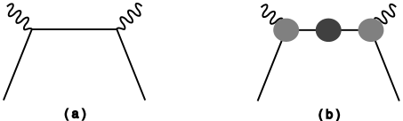
FIG. 5.: Photon-nucleon Compton diagrams in fully relativistic formalism: a) the nucleon-pole diagram; b) a one-particle reducible diagram.

Obviously, conventional HB$\chi$PT fails at this special kinematic point because the nucleon propagator in a 1PR diagram, $1/\nu$, is divergent. When this happens, one has to sum over all 1PR diagrams to get a “nonperturbative” contribution. In what follows, we are going to argue that all such divergent contributions just add up to the nucleon elastic contribution which we know how to calculate independently of HB$\chi$PT.

Let us consider a generic $s$-channel 1PR diagram shown in Fig. 5b in the usual fully-relativistic chiral perturbation theory. The structure of the diagram is

$$\Gamma^{\mu}(\nu,Q^{2})S_{N}(P+q)\tilde{\Gamma}^{\nu}(\nu,Q^{2})\ ,$$ (28)

where the $\Gamma$’s represent the three-point nucleon-photon vertex functions and $S_{N}(P+q)$ is the dressed nucleon propagator. To isolate the singular contribution, let us expand the $\Gamma$’s and the nucleon propagator at $\nu=Q^{2}/2M$, i.e., the onshell kinematic point for the intermediate nucleon propagator. All terms are regular as $\nu$ and $Q^{2}\rightarrow 0$, except for the following

$$\left.\Gamma^{\mu}(\nu,Q^{2}){i\over\not\!P+\not\!q-M}\tilde{\Gamma}^{\nu}(\nu,Q^{2})\right|_{\nu=Q^{2}/2M}\ .$$ (29)

It is quite clear that $\Gamma(\nu=Q^{2}/2M,Q^{2})$’s are just the matrix elements of the electromagnetic currents between the on-shell nucleon states. Therefore all singular contributions are from the nucleon elastic scattering.

When all such singular contributions from $s$- and $u$-channel are summed, we find, for instance,

$$S_{1}^{\rm el}(\nu,Q^{2})=-2F_{1}(Q^{2})\left(F_{1}(Q^{2})+F_{2}(Q^{2})\right)\left[{1\over 2M\nu-Q^{2}}-{1\over 2M\nu+Q^{2}}\right]\ ,$$ (30)

where $F_{1}(Q^{2})$ and $F_{2}(Q^{2})$ are the nucleon form factors in chiral perturbation theory. When setting $\nu=0$, we have a perfectly finite result. However, when expanded in $1/\nu$ as one does in HB$\chi$PT, it produces $(1/\nu)^{n}(n=1,2,...)$ singularities.

Therefore, there is no need to calculate the $1/\nu$-type singular contributions in HB$\chi$PT. To account for them, one just calculates the Dirac and Pauli form factors and substitutes them in Eq. (30). In the end the recipe for $S_{1,2}(0,Q^{2})$ becomes very simple: Consider a Feynman diagram and calculate it at finite $\nu$ using the rules in HB$\chi$PT. Expand the result in a Laurent series about $\nu=0$, and keep only the $\nu$-independent constant term. Add the nucleon elastic contribution.

One final point about the HB$\chi$PT formalism. In the fully-relativistic calculation presented in Sec. III, all Feynman diagrams contribute to $S_{1}(0,0)$ at order $M^{0}$, and the sum is zero because of electromagnetic gauge invariance. It turns out, however, none of these diagrams contributes at this order in HB$\chi$PT. When examing the relativistic calculation carefully, we find that the order-$M^{0}$ contribution comes from the high-momentum region $k\sim M$ of the loop integrals. In HB$\chi$PT, the leading contribution is nominally of order-$1/M$ multiplied by linearly-divergent integrals. These integrals can produce order-$M^{0}$ contributions in a cut-off regularization. In dimensional regularization, however, the linearly-divergent pieces are set to zero by hand. This is allowed in field theory because different regularization schemes can differ by innocuous constants which are finally fixed by renormalization conditions. In the present case HB$\chi$PT does not need to reproduce, diagram by diagram, the constant contributions to $S(0,0)$ in a fully- relativistic calculation. The only constraint is the low-energy theorem.

VI Extended Test of Chiral Pertubation Theory

Chiral perturbation theory extends the low-energy theorems and makes general predictions of the spin-dependent foward Compton amplitudes $S_{1,2}(\nu,Q^{2})$ in a kinematic region where $\nu$ and $Q^{2}$ are much smaller than the hadron mass scale. The predictions, in particular the $\nu$-dependence, can be tested against experimental data on the spin-dependent structure functions $G_{1,2}(\nu,Q^{2})$ through the dispersion relations. Notice that $\nu$ in the Compton amplitudes is not the same as the virtual photon-energy in $G_{1,2}(\nu,Q^{2})$. The former $\nu$ must be kept small in order to justify a calculation in chiral perturbation theory, whereas the $\nu$-dependence of the structures functions must in principle cover the full kinematic range $0<\nu<\infty$ in order to construct the dispersion integral.

One can think of two ways to test the $\nu$ dependence. First, expand $S_{1}(\nu,Q^{2})$ and $S_{2}(\nu,Q^{2})$ as Taylor series around $\nu=0$,

$$S_{1}(\nu,Q^{2}) = \sum_{n=0,2,4,...}\nu^{n}S_{1}^{(n)}(Q^{2})\ ,$$ (31)

$$S_{2}(\nu,Q^{2}) = \sum_{n=1,3,5,...}\nu^{n}S_{2}^{(n)}(Q^{2})\ .$$ (32)

Using the dispersion relations in Eq. (12), we find that the coefficients $S_{1}^{(n)}(Q^{2})$ and $S_{2}^{(n)}(Q^{2})$ define two infinite towers of dispersive sum rules,

$$S_{1}^{(n)}(Q^{2}) = 4\int^{\infty}_{Q^{2}/2M}{d\nu\over\nu^{n+1}}G_{1}(\nu,Q^{2})~{}~{}~{}~{}(n=0,2,4,...)\ ,$$ (33)

$$S_{2}^{(n)}(Q^{2}) = 4\int^{\infty}_{Q^{2}/2M}{d\nu\over\nu^{n+1}}G_{2}(\nu,Q^{2})~{}~{}~{}~{}(n=1,3,5,...)\ .$$ (34)

These sum rules are certainly familar in the context of deep-inelastic scattering [29]. The point we want to make here is that they can be extended to low-$Q^{2}$ using the predictions for $S_{1,2}^{(n)}(Q^{2})$ from chiral perturbation theory. In fact, the $S_{1}^{(2)}(Q^{2})$ sum rule extends the known spin-dependent-polarizability sum rule at $Q^{2}=0$ to arbitrary $Q^{2}$ [30].

The second way to test the $\chi$PT predictions is to directly compare the theoretical $S_{1,2}(\nu,Q^{2})$ with the extracted Compton amplitudes from data on $G_{1,2}(\nu,Q^{2})$. We will argue below that this method has an important advantage over the first one.

We have calculated the full $Q^{2}$- and $\nu$-dependent $S_{1,2}(\nu,Q^{2})$ at leading-order in $\chi$PT. With the nucleon intermediate states, we need to consider only three of the diagrams shown in Fig. 3 ($(d)$, $(h)$, and $(i)$). The result is

$${\overline{S}_{1}}^{N}(\nu,Q^{2})=8\left({g_{A}\over 4\pi f_{\pi}}\right)^{2}\int^{1}_{0}dx\left({\tilde{m}_{\pi}\over\nu}\right)\left[\left(1-\left({x\nu\over\tilde{m}_{\pi}}\right)^{2}\right)^{-1/2}\sin^{-1}\left({x\nu\over\tilde{m}_{\pi}}\right)-{x\nu\over\tilde{m}_{\pi}}\right]\ .$$ (35)

For $x\nu>\tilde{m}_{\pi}$, one must analytically continue the inverse sine function and the square roots. Giving an infinitesimal positive imaginary part to $\nu$ yields

$${\sin^{-1}x\over\sqrt{1-x^{2}}}\rightarrow{\ln(x-\sqrt{x^{2}-1})+i{\pi/2}\over\sqrt{x^{2}-1}}\ .$$ (36)

As expected, the Compton amplitudes develope imaginary parts for $\nu>m_{\pi}$, due to the physical production of the $\pi N$ state. The $\Delta$ contribution comes in in two different ways: First through the pole diagram in Fig. 4a

$$S_{1}^{\Delta,\rm dir}(\nu,Q^{2})={1\over 9}\left(G_{1}\over M\right)^{2}\nu\left[{1\over\nu-\Delta+i{\Gamma_{\Delta}/2}}+{1\over\nu+\Delta-i{\Gamma_{\Delta}/2}}\right]\ ,$$ (37)

where $G_{1}$ is the $\gamma$-$\Delta$-$N$ coupling (don’t confuse with the structure function $G_{1}(\nu,Q^{2})$!) and $\Gamma_{\Delta}$ is the width of the $\Delta$. In the large-$N_{c}$ limit, $G_{1}=(3/\sqrt{2})\kappa_{V}$ where $\kappa_{V}$ is the (dimensionless) isovector anomalous magnetic moment of the nucleon. The $\Delta$ also contributes via the one-loop intermediate states in Figs. 4b, 4c, and 4d. We find

$$S_{1}^{\Delta}(\nu,Q^{2}) = 2\left({4\over 3}\right)^{2}\left({g_{\pi N\Delta}\over 4\pi f_{\pi}}\right)^{2}\int^{1}_{0}dx\,\,\left[x+{\tilde{m}_{\pi}\over\nu}\left(1-{\Delta\tilde{\nu}\over\tilde{m}_{\pi}^{2}}\right)\right.$$ (39)

$$\times\left.\left(1-{\tilde{\nu}^{2}\over\tilde{m}_{\pi}^{2}}\right)^{-1/2}\left(\sin^{-1}\left({\tilde{\nu}\over\tilde{m}_{\pi}}\right)-{\pi\over 2}\right)\right]+(\nu\rightarrow-\nu)\,\,\,,\$$

where $\tilde{\nu}=\Delta-x\nu$ and $\Delta=M_{\Delta}-M$. This amplitude is real when $\nu$ is below the pion-$\Delta$ production threshold ($<\Delta+m_{\pi}$). Once again, the $\Delta$-loop contribution cancels the nucleon contribution in the large-$N_{c}$ limit, and the cancellation reflects the contracted $SU(4)$ spin-flavor symmetry of the large-$N_{c}$ QCD [27, 28]. In the real photon limit $Q^{2}=0$, our result reproduces that in Ref. [23]. In Fig. 6a, we have shown the real part of the ${\overline{S}_{1}}(\nu,Q^{2})$ amplitude in a three-dimensional plot. Here, we have used $g_{A}=1.26$ and the large-$N_{c}$ values $g_{\pi N\Delta}=3/(2\sqrt{2})g_{A}$ and $G_{1}=(3/\sqrt{2})\kappa_{V}$. The $\Delta$ resonance contribution has been included explicitly. For the physical $\Delta$ mass, we find the contribution is small execept near the $\Delta$ resonance.

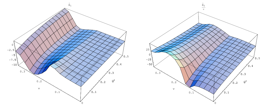
FIG. 6.: (${\it Left}$) ${\overline{S}_{1}}(\nu,Q^{2})\,\,({\rm GeV}^{-2})$ and (${\it Right}$) ${\overline{S}_{2}}(\nu,Q^{2})/\nu\,\,({\rm GeV}^{-4})$ at leading order in chiral perturbation theory. $Q$ and $\nu$ are in GeV’s. We note the N-$\pi$ and $\Delta$ resonances at $\nu=0.14\,{\rm GeV}$ and $0.28\,{\rm GeV}$, respectively.

We now turn to the result for $S_{2}(\nu,Q^{2})$. From the one-loop diagrams with a nucleon intermediate state, we find

$${\overline{S}_{2}}^{N}(\nu,Q^{2})=4\left({g_{A}\over 4\pi f_{\pi}}\right)^{2}\int^{1}_{0}dx{x(1-2x)\over\tilde{m}_{\pi}}\left(1-\left({x\nu\over\tilde{m}_{\pi}}\right)^{2}\right)^{-1/2}\sin^{-1}\left({x\nu\over\tilde{m}_{\pi}}\right)\ ,$$ (40)

which is odd in $\nu$. An imaginary part develops as $\nu$ passes over the pion-production threshold. The contribution from the direct $\Delta$ production gives

$$S_{2}^{\Delta,\rm dir}(\nu,Q^{2})=-{1\over 9}\left(G_{1}\over M\right)^{2}\left[{1\over\nu-\Delta+i{\Gamma_{\Delta}/2}}+{1\over\nu+\Delta-i{\Gamma_{\Delta}/2}}\right]\ .$$ (41)

The one-loop diagrams with the $\Delta$ as an intermediate state give

$$S_{2}^{\Delta}(\nu,Q^{2}) = \left({4\over 3}\right)^{2}\left(g_{\pi N\Delta}\over 4\pi f_{\pi}\right)^{2}\int^{1}_{0}dx{x(1-2x)\over\tilde{m}_{\pi}}\left(1-{\tilde{\nu}^{2}\over\tilde{m}_{\pi}^{2}}\right)^{-1/2}$$ (43)

$$\times\left[\sin^{-1}\left({\tilde{\nu}\over\tilde{m}_{\pi}}\right)-{\pi\over 2}\right]-(\nu\rightarrow-\nu)\ .$$

In the large-$N_{c}$ limit, the nucleon and $\Delta$ contribution cancel. In Fig. 6b, we have shown a three-dimensional plot of ${\overline{S}_{2}}(\nu,Q^{2})/\nu$.

Because of the existence of the inelastic thresholds, the Taylor-expansion of $S_{1,2}(\nu,Q^{2})$ at $\nu=0$ breaks down at the nearest singularity $\nu\sim m_{\pi}$. This is reflected by terms of order $(\nu/m_{\pi})^{n}$ in the $\nu$-expansion. Therefore, $S_{1,2}^{(n)}(Q^{2})$ are strongly singular and very large even for a realistic pion mass. This is the reason that the sum rules in Eq. (34) are not the best way to test the $\chi$PT predictions. Indeed, the validity of a chiral expansion is not limited to $\nu<m_{\pi}$. The terms that we neglect in our calculation are of order $m_{\pi}/M$, $\nu/M$, and $Q^{2}/M^{2}$. The chiral expansion is not really a Taylor expansion in $\nu$; the generic structure of this expansion looks like

$$S(\nu)=\sum_{n=0}^{\infty}{\left(\nu\over M\right)}^{n}C_{n}(\nu/m_{\pi})\ ,$$ (44)

where we have neglected $Q^{2}$ and set $4\pi f_{\pi}=M$ to illustrate the point. While the coefficient $C_{n}(x)$ has a zero radius of convergence when expanded in the chiral limit, the chiral expansion in different orders of $\nu/M$ makes perfect sense.

VII How does Drell-Hearn-Gerasimov meet Bjorken?

Consider the nucleon structure functions $G_{1,2}(\nu,Q^{2})$ in the deep-inelastic region: $Q^{2}\rightarrow\infty$, $\nu\rightarrow\infty$, and the ratio staying fixed. A well-known sum rule for $g_{1}^{p-n}(\nu,Q^{2})=M\nu G_{1}^{p-n}(\nu,Q^{2})$ at $Q^{2}=\infty$ was first derived by Bjorken using the current algebra method [9]. In fact, Bjorken derived the more general sum rules which are separately valid for a proton or neutron target:

$$\Gamma^{p(n)}(Q^{2}) \equiv \int^{1}_{0}g_{1}^{p(n)}(x,Q^{2})dx$$ (45)

$$\rightarrow \pm{1\over 12}g_{A}+{1\over 36}g_{8}+{1\over 9}g_{0}$$ (46)

as $Q^{2}\rightarrow\infty$, where $g_{A}$, $g_{8}$, and $g_{0}$ are the nucleon matrix elements of the axial currents $A^{\mu}_{a}$ $(a=3,8,0)$,

$$\langle PS|A^{\mu}_{a}(0)|PS\rangle=g_{a}(2S^{\mu}).$$ (47)

The matrix element $g_{A}$ is precisely known from neutron-$\beta$ decay, and $g_{8}$ may be extracted from hyperon-$\beta$ decay if chiral SU(3) symmetry in under control[28]. The simple quark model predicts $g_{0}\equiv\Delta\Sigma=1$. Ellis and Jaffe assumed $\Delta\Sigma=g_{8}$ based on the empirical observation that the strange quarks play an insignificant role in nucleon structure [31]. Ellis and Jaffe’s estimate for the right-hand side of Eq. (46) has been called the Ellis-Jaffe sum rule. We note that the Bjorken sum rule can also be derived using the modern technique of operator product expansions in QCD.

To reconcile the discrepency between the EMC extraction of $\Delta\Sigma$ at ${\overline{Q}^{2}}=10$ GeV² from the polarized deep-inelastic scattering data and the simple quark model prediction, Anselmino et al. observed that the $g_{1}^{p}(x,Q^{2})$ integral at finite $Q^{2}$ can have significant deviation from the Bjorken’s prediction [32]. Their argument is as follows: Consider the $Q^{2}$-dependence of the integral

$$I(Q^{2}) \equiv \int^{\infty}_{Q^{2}/2M}M^{2}G_{1}(\nu,Q^{2})d\nu/\nu$$ (48)

$$= {2M^{2}\over Q^{2}}\Gamma(Q^{2})\ .$$ (49)

As $Q^{2}\rightarrow\infty$, the Bjorken sum rule indicates that $I^{p}(Q^{2})$ approaches zero from above. On the other hand, the DHG sum rule says $I^{p}(0)=-\kappa^{2}_{p}/4$, large and negative. Therefore, $I(Q^{2})$ must undergo a rapid variation from $Q^{2}=\infty$ to 0. This variation could imply a significant deviation of the the EMC data at ${\overline{Q}^{2}}=10$ GeV² from the Bjorken sum rule at $Q^{2}=\infty$. They devised a simple phenomenological model to illustrate this.

As pointed out by one of us [34] and explained in more depth below, Anselmino et al.’s observation is misleading in its original intent. However, undertanding the $Q^{2}$-evolution of $\Gamma(Q^{2})$ or $I(Q^{2})$ over the full range of $Q^{2}$ is interesting in itself. We will argue below that the $Q^{2}$-dependence can largely be understood in terms of chiral perturbation theory at low $Q^{2}$ and the operator production expansion at high $Q^{2}$. There exists, however, a small intermediate-$Q^{2}$ window where the transition from hadron to parton degrees of freedom occurs and where we do not yet have a firm theoretical handle. Future precise experimental data in this region could help us to understand how the parton-hadron transition happens.

In the definition of the $I(Q^{2})$ integral in Ref. [32], the lower integration limit indicates that the nucleon elastic contribution was included. However, since the elastic contribution is absent at $Q^{2}=0$, overwhelming at small $Q^{2}$, and finally becomes negligible at high $Q^{2}$, $I(Q^{2})$ cannot vary continuously from $Q^{2}=0$ to $\infty$ unless the elastic contribution is subtracted. Therefore, the $Q^{2}$-evolution picture considered by Anselmino et al. does not actually include the elastic contribution. For a quanity integrating over inelastic contributions only, there is no twist expansion, and hence one cannot say anything about the size of the twist-four matrix element from Anselmino et. al.’s simple phenomenological model. The same comment applies to Ref. [33].

To really understand the $Q^{2}$-evolution of $I(Q^{2})$ from $Q^{2}=0$ to $\infty$, we again consider the $Q^{2}$-dependent dispersive sum rule,

$$S_{1}(0,Q^{2})=4\int^{\infty}_{Q^{2}/2M}{d\nu\over\nu}G_{1}(\nu,Q^{2})\ ,$$ (50)

which, as emphasized above, is the origin of the generalized DHG sum rule and the Bjorken sum rule. Consequently,$I(Q^{2})$ or $\Gamma(Q^{2})$ as a function of $Q^{2}$ can be obtained just from the Compton amplitude $S_{1}(0,Q^{2})$. Since the available theoretical methods, such as chiral perturbation theory, operator product expansion, or lattice QCD are natural tools for calculating $S_{1}(0,Q^{2})$, it is natural to consider the $G_{1}$-integral including the elastic contribution. We know of no way to directly calculate ${\overline{S}_{1}}(0,Q^{2})$ other than using the definition ${\overline{S}_{1}}(0,Q^{2})\equiv S_{1}(0,Q^{2})-S_{1}^{\rm el}(0,Q^{2})$.

Once the elastic contribution is included, we see that it dominates $S_{1}(0,Q^{2})$ at low $Q^{2}$ because of the $1/Q^{2}$ singularity. Since $S_{1}(0,Q^{2})$ contains the same $1/Q^{2}$ factor at asymptotic $Q^{2}$, it is convenient to study just the $Q^{2}$ evolution of

$$\Gamma(Q^{2})={Q^{2}\over 8}S_{1}(0,Q^{2})\ ,$$ (51)

It interesting to note that for a pointlike proton, $\Gamma(Q^{2})$ is simply 1/2, independent of $Q^{2}$.

In the $Q^{2}=\infty$ to $0.5$ GeV² region, $\Gamma(Q^{2})$ can be obtained essentially from parton physics formalized in the operator product expansion. From the OPE for the Compton amplitude $S_{1}(0,Q^{2})$, we can write

$$\Gamma(Q^{2})=\sum_{\tau=2,4,...}{\mu_{\tau}(Q^{2})\over(Q^{2})^{(\tau-2)/2}}\ ,$$ (52)

where $\mu_{\tau}$ itself is a perturbation series in $\alpha_{s}(Q^{2})$. For instance [10]

$$\mu_{2}(Q^{2}) = \left(1-{\alpha_{s}\over\pi}-3.58\left({\alpha_{s}\over\pi}\right)^{2}-20.22\left({\alpha_{s}\over\pi}\right)^{3}\right)\left(\pm{g_{A}\over 12}+{a_{8}\over 36}\right)+$$ (54)

$$+\left(1-0.33{\alpha_{s}\over\pi}-0.55\left({\alpha_{s}\over\pi}\right)^{2}-4.45\left({\alpha_{s}\over\pi}\right)^{3}\right){\Delta\Sigma\over 9}+{\cal O}(\alpha_{s}^{4}).$$

The $\mu_{4}$ correction has been expressed in terms of various nucleon matrix elements [35]. No one has yet worked out the local operators associated with $\mu_{6}$. The physical significance of the twist expansion is that at large $Q^{2}$, the Compton amplitude can be understood in terms of the scattering of a few partons.

What is the physical scale parameter which controls the twist expansion? By studying the structure of higher-twist operators, one finds that the relevant dimensional parameter is the average parton transverse momentum in the nucleon [36]. On dimensional grounds, one can write

$$\mu_{\tau}\sim\langle k_{\perp}\rangle^{\tau-2}\ .$$ (55)

The numerical size of $\langle k_{\perp}\rangle$ is believed to be around 0.4 to 0.5 GeV. Therefore, the naive expectation is that the $1/Q^{2}$-expansion is a good approximation down to $Q^{2}\sim 0.5$ GeV². This picture is in fact consistent with the experimental data. As $Q^{2}$ changes from $0.5$ to $\infty$, the $x$-dependence of the $g_{1}(x,Q^{2})$ scaling function changes significantly. However, its first moment, $\Gamma(Q^{2})$, is nearly independent of $Q^{2}$, as required by the twist expansion. In Ref. [37], the twist-four matrix elements were extracted from the $Q^{2}$ dependence of data on $\gamma(Q^{2})$. In Fig. 7a, we have plotted the evolution of $\Gamma(Q^{2})$ for the proton with the twist-two and twist-four contributions included ($\mu^{p}_{4}$ is taken to be 0.04 GeV²).

At low $Q^{2}$, the elastic contribution dominates $\Gamma(Q^{2})$, which approaches $e(1+\kappa)/2$ as $Q^{2}\rightarrow 0$. As $Q^{2}$ deviates from zero, $\Gamma(Q^{2})$ falls rapidly due to the nucleon elastic form factor. The leading inelastic contribution appears as a linear term in $Q^{2}$ and the slope can be obtained from the DHG sum rule. The sign of this slope enhances the rapid decrease of the elastic contribution. Chiral perturbation theory allows us to compute the $Q^{2}$ dependence of the inelastic contribution as a perturbation series in $Q^{2}$

$${\overline{\Gamma}}(Q^{2})=-{\kappa^{2}Q^{2}\over 8M^{2}}+{\cal O}\left({Q^{4}\over((4\pi f_{\pi})^{2}Mm_{\pi})}\right)\ .$$ (56)

The total $Q^{2}$ variation is

$$\Gamma(Q^{2})={1\over 2}F_{1}(Q^{2})\left(F_{1}(Q^{2})+F_{2}(Q^{2})\right)+{\overline{\Gamma}}(Q^{2})\ .$$ (57)

In Fig. 7a, we have plotted the elastic contribution as the dashed curve and the elastic plus the leading term in ${\overline{\Gamma}}(Q^{2})$ as a solid curve. Adding higher-order chiral corrections will bring changes to the solid curve. However, chiral power counting guarantees that the change in the $Q^{2}$ range between 0 to approximately $0.2$ GeV² will be relatively small. Therefore, we believe that the description of $\Gamma(Q^{2})$ in terms of the hadron degrees of freedom will be trustable at least up to $Q^{2}=0.2$ GeV².

FIG. 7.: ${\it Left}$ : $Q^{2}$-evolution of the $\Gamma(Q^{2})$ integral studied from the Compton amplitude $S_{1}(0,Q^{2})$. ${\it Right}$ : The subtracted integral ${\overline{I}}(Q^{2})$.

As Fig. 7a shows, the $Q^{2}$-dependence of $\Gamma^{p}(Q^{2})$ can already be understood over a large kinematic region in terms of chiral perturbation theory and the twist expansion. Mathematically, there is little left to the imagination between $Q^{2}=0.2$ and 0.5 GeV² other than a smooth curve connecting the high and low-$Q^{2}$ regions. Physically, however, the missing link is very interesting. This is the regime in which the transition between parton and hadron degrees of freedom happens and so it provides an important ground on which to test ideas about how the transition occurs. There is a possibility that chiral perturbation theory and the twist-expansion with the appropriate inclusion of higher-order terms (e.g. pade approximation, resonance dominance, etc. ) are simultaneously valid in an overlapping region. This scenario has been the main theoretical condition for the validity of QCD sum rule calculations [38]. Alternatively, it is possible that there is an open window in which neither theory works. In this case, one must consider other methods, such as lattice QCD. It is interesting to note that $S_{1}(0,Q^{2})$ can in fact be calculated in lattice QCD by rotating the Minkowski time in Eq. (6) to Euclidean.

The global $Q^{2}$-variation of $\Gamma(Q^{2})$ reveals a simple and appealing physical picture. When the photon momentum is low, it scatters coherently over all the constituents of the nucleon and the response shows a diffractive type of peak which stands well above the pointlike value of 1/2. When $Q^{2}$ is large, the photon sees the individual quarks in the nucleon and the scattering is an incoherent sum of all charged constituents. Thus, $\Gamma(Q^{2})$ is necessarily much smaller than 1/2. In fact, it will asymptotically vanish if the proton contains no pointlike particles but a smeared charge distribution. The transition between the whole proton and its constituent scattering happens at $Q^{2}$ corresponding roughly to the size of the system.

The only unattractive feature of Fig. 7a is that the elastic contribution at low $Q^{2}$ overwhelms the inelastic contribution, making the transition region less dramatic. Therefore, we plot in Fig. 7b the $Q^{2}$-dependence of the subtracted integral ${\overline{I}}(Q^{2})$, as suggested by Anselmino et al. Now, we see the our leading chiral prediction becomes a straight line which we draw up to 0.2 GeV². On the high-$Q^{2}$ side, we find that ${\overline{I}}(Q^{2})$ crosses from positive to negative at $Q^{2}\sim 0.6$ GeV². The significance of this crossing point is that it is where the elastic contribution equals the prediction of the leading twist expansion. Below this $Q^{2}$, the curve dives down to meet the low-energy theorem $(-\kappa^{2}/4)$ and its chiral extension. Therefore, while the detail may vary (the crossing point is likely less than 0.5 GeV² according to E143 data [1]), the seemingly intriguing $Q^{2}$ variation of ${\overline{I}}(Q^{2})$ near the crossing point is nothing but a simple consequence of an innocent construct. The higher-order corrections in chiral perturbation theory and the twist-expansion may provide a more accurate account of how the Drell-Hearn-Gerasimov sum rule finally meets that of Bjorken.

VIII Summary and Outlook

In this paper, we have studied generalized sum rules for the spin-dependent structure functions of the nucleon. We emphasize that to obtain sum rules, one has to find ways to calculate the virtual-photon forward Compton amplitudes $S_{1,2}(\nu,Q^{2})$.

Away from the $\nu=Q^{2}=0$ point where there is a well-known low-energy theorem, one can use chiral perturbation theory to calculate the $\nu$ and $Q^{2}$ dependence. We find that for $S_{1}(0,Q^{2})$ the leading chiral contribution vanishes because of the spin symmetry of the heavy-nucleon limit. The result from the next-order $\chi$PT calculation, for example, the coefficient of the $Q^{2}/(Mm_{\pi}(4\pi f_{\pi})^{2})$ term, will be published elsewhere [26]. Our result for ${\overline{S}_{2}}^{(1)}(0,Q^{2})$ yields a new sum rule for the $G_{2}(\nu,Q^{2})$ structure function. The complete $Q^{2}$ and $\nu$ dependence of the low-energy Compton amplitudes can be tested through standard dispersion relations.

For large $Q^{2}$, the Compton amplitudes can be expressed as a power series in $1/Q^{2}$ following an operator product expansion of the electromagnetic currents. We emphasize that this is possible only for the complete amplitudes including the nucleon elastic contribution. For $S_{1}(0,Q^{2})$, the twist expansion is expected to converge for $Q^{2}>0.5$ GeV². Using dispersion relations, the Bjorken sum rule can be generalized approximately down to this $Q^{2}$.

Therefore, the low-energy $Q^{2}$ dependence of $S_{1}(0,Q^{2})$ and the related sum rule can be described in terms of the physics of the hadron degrees of freedom, whereas the high-energy dependence can be described in terms of parton degrees of freedom. According to what we know of both theories, there is only a small $Q^{2}$ window in which we have no solid theoretical understanding. Clearly, precise experimental data in this region will allow us to understand how the transion from parton to hadron degrees of freedom happens. On the theoretical side, it is important to pursue higher-order corrections in chiral perturbation theory and the twist expansion. Ultimately, a precision lattice QCD calculation may help establish the final missing link between the DHG and Bjorken sum rules.