CERN-TH/99-109
hep-ph/9905403 DESY 98-199
Measuring Gauge-Mediated SuperSymmetry Breaking
Parameters at a 500 GeV Linear Collider
Sandro Ambrosanio a,c and Grahame A. Blair b,c
a CERN – Theory Division,
CH-1211 Geneva 23, Switzerland (current address)
e-mail: ambros@mail.cern.ch
b Royal Holloway and Bedford New College,
University of London, Egham Hill, Egham,
Surrey TW20 0EX, U.K. (current address)
e-mail: g.blair@rhbnc.ac.uk
c Deutsches Elektronen-Synchrotron DESY,
Notkestraße 85, D-22603 Hamburg, Germany
Abstract
We consider the phenomenology of a class of gauge-mediated supersymmetry (SUSY) breaking (GMSB) models at a Linear Collider (LC) with up to 500 GeV. In particular, we refer to a high-luminosity ( cm-2 s-1) machine, and use detailed simulation tools for a proposed detector. Among the GMSB-model building options, we define a simple framework and outline its predictions at the LC, under the assumption that no SUSY signal is detected at LEP or Tevatron. We assess the potential of the LC to distinguish between the various SUSY model options and to measure the underlying parameters with high precision, including for those scenarios where a clear SUSY signal would have already been detected at the LHC before starting the LC operations. Our focus is on the case where a neutralino () is the next-to-lightest SUSY particle (NLSP), for which we determine the relevant regions of the GMSB parameter space. Many observables are calculated and discussed, including production cross sections, NLSP decay widths, branching ratios and distributions, for dominant and rare channels. We sketch how to extract the messenger and electroweak scale model parameters from a spectrum measured via, e.g. threshold-scanning techniques. Several experimental methods to measure the NLSP mass and lifetime are proposed and simulated in detail. We show that these methods can cover most of the lifetime range allowed by perturbativity requirements and suggested by cosmology in GMSB models. Also, they are relevant for any general low-energy SUSY breaking scenario. Values of as short as 10’s of m and as long as 10’s of m can be measured with errors at the level of 10% or better after one year of LC running with high luminosity. We discuss how to determine a narrow range () for the fundamental SUSY breaking scale , based on the measured , . Finally, we suggest how to optimise the LC detector performance for this purpose.
⋆ To be published in The European Physical Journal C
1 Introduction
If the world is supersymmetric at short distances, then the gauge hierarchy problem can be naturally solved. The most compelling proof of this hypothesis would be direct detection of superpartners at colliders. This has not been achieved so far, which tells us that supersymmetry (SUSY) must be broken. In order for a SUSY theory to preserve its theoretically pleasant characteristics, supersymmetry breaking (SSB) can only occur in a “soft” way [1]. However, this constraint still allows a general phenomenological approach to SSB involving over a hundred new parameters in addition to the Standard Model (SM) ones. Strategies for searches at present and future colliders must then rely, at least to start with, on theoretically well-motivated schemes for SSB, providing a more definite framework and living on a manageable parameter space. A related question is how this SSB is transmitted to the visible (light) sector of the theory, e.g. the particles of the Minimal SUSY extension of the SM (MSSM). Historically, the most popular approach has been that SUSY is broken at very high energies (HESB) of the order of the Planck mass or the scale of Grand-Unified Theories (GUT) and SSB is communicated to the MSSM sector through gravitational interactions. Such an approach goes usually under the name of (minimal) Supergravity [(m)SUGRA] or, with some additional assumptions, Constrained MSSM (CMSSM) [2]. More recently, another equally attractive scenario has earned large consensus and recognition, both among theorists and experimentalists, the Low-Energy Supersymmetry Breaking (LESB) option, and in particular, the Gauge-Mediated (GMSB) version of it [3]. LESB, in itself, may already have striking phenomenological consequences, as it was shown in pioneering works by Fayet [4]. Indeed, gravity enters the expression for the gravitino mass,
| (1) |
where is the fundamental scale of SSB, 100 TeV is a typical value for it in LESB models, and GeV is the reduced Planck mass. As a result, the gravitino is so light in LESB models that it plays always the rôle of the lightest SUSY particle (LSP) and can be treated as massless for all kinematics purposes at high energy colliders. However, for , the dominant gravitino interactions come from its longitudinal, spin-1/2 components, namely the goldstino components that the gravitino has acquired through the so-called SUSY-Higgs mechanism. Hence, gravity does not enter the strength of the gravitino couplings to matter, which in the relevant approximation are proportional to the mass splitting between superpartner masses and the ordinary SM particle masses and inversely proportional to . The latter can be small enough to render the gravitino relevant for collider phenomenology. (It should be noted here that a light gravitino LSP can also be obtained within the framework of no-scale SUGRA models [5].)
The phenomenological scenario in LESB with conserved -parity (which we assume in the rest of the paper) can be summarised as follows:
-
•
every produced SUSY particle has to decay to the , possibly through a cascade;
-
•
since the goldstino interactions are still much weaker than the ordinary SM gauge and Yukawa interactions, every decay chain has to involve the next-to-lightest SUSY particle (NLSP), which in turn will finally decay to the gravitino;
-
•
depending on , the production energy and details of the SUSY spectrum, the NLSP can decay close to the interaction point (i.p.), within or outside a collider detector, producing a plethora of new spectacular signatures.
Among the possible mechanisms for transmitting LESB to the MSSM fields, by far the most effective and theoretically satisfying is GMSB, where a so-called messenger sector is responsible for communication between the secluded sector where SSB takes place and the visible sector, via SM gauge interactions. Mainly motivated by a natural suppression of the SUSY contributions to flavour-changing neutral current (FCNC) and CP-violating processes, such a scenario was first explored in various forms in several early 1980’s works [6] and then recently revived in its present version in the famous papers of Ref. [7]. Remarkably, in addition to the appealing theoretical features, the minimal version of GMSB also provides a powerful tool for building very predictive models and calculating spectra from just a handful of parameters, as done e.g. in Refs. [8, 9, 11]. An important boost to the popularity of LESB and GMSB models came a few years ago due to a possible explanation of the anomalous CDF event within this framework [12, 13]. Today, such an explanation seems more unlikely, yet it worked fine in stimulating a considerable number of dedicated analyses and searches for GMSB-inspired new signals at LEP and Tevatron, which are of course of much broader interest [12, 14, 15]. Hence, it is now time to think about how similar searches could be pursued at next generation colliders and how the reach in the GMSB parameter space of such machines could be optimised. Some work in this respect has already been carried out for the Tevatron Run II [16] and for the LHC [17]. In this paper, we will be instead mainly concerned with GMSB phenomenology at a first phase of operations of a Linear Collider (LC) with c.o.m. energy up to around 500 GeV, and will focus on the case where a neutralino is the NLSP. In particular, we will refer to a high-luminosity machine with cm-2 s-1, such as being considered e.g. by the ECFA/DESY TESLA project, and the related proposed detector. Many of our results and experimental methods can be easily extended to more general LESB models and might even have an impact on other scenarios such as HESB models with -parity violation, where delayed NLSP or LSP decays can take place.
The rest of this paper is organised as follows. In Sec. 2, we briefly describe our GMSB-model building framework and specify the region of the parameter space we are interested in here. In Sec. 3, we focus on the general phenomenology of models with a neutralino NLSP and discuss its possible (delayed) decays, including some new aspects of interest for the LC. In Sec. 4, we introduce the main features of the proposed TESLA linear collider and give the expected machine parameters relevant to our study. In Sec. 5, we discuss the general characteristics of the GMSB signal at the LC and show an example of how it is possible to extract a good amount of information about the GMSB parameters via a simple experimental technique in principle possible at such a machine. In Sec. 6, we describe the relevant characteristics of the LC detector and the software we used for our simulations. In Sec. 7, we discuss several methods for measuring the neutralino NLSP properties, and in particular its mass and lifetime, using different parts of the detector, and we show our results. Finally, in Sec. 8, we draw our conclusions and comment on how the performance of the LC in measuring GMSB parameters depends on details of the machine and detector design. We also give a few suggestions to optimise such performance.
2 Models with Gauge-Mediated SUSY Breaking
In addition to the automatic suppression of SUSY FCNC, GMSB models have many other interesting characteristics. For instance, the sparticles’ masses have a transparent and common origin and all approximately scale with a single parameter which is the universal soft SUSY breaking scale for the visible sector. Also, the resulting spectrum is notably different from other SUSY scenarios. Further, it is possible to achieve radiative electroweak symmetry breaking (EWSB) nicely. There are however problems connected for instance with the lack of a compelling dynamical mechanism for generating the SUSY parameter , but this is common to other SUSY frameworks.
As far as GMSB-model building is concerned, we will follow closely the approach used in Ref. [11] for LEP2 phenomenology, with some extensions of the parameter space to account for the wider kinematical reach of a LC. We will not repeat the technical details here, but in order to fix our framework and notations we remind that, after imposing EWSB, a minimal GMSB model can be constructed from the following parameters,
| (2) |
where is the overall messenger scale; is the so-called messenger index that parameterises the structure of the messenger sector; is the universal soft SUSY breaking scale felt by the low-energy sector; is the ratio of the vacuum expectation values (VEVs) of the two Higgs doublets; sign() is the ambiguity left for the SUSY higgsino mass after EWSB conditions are imposed. The MSSM parameters and the sparticle spectrum are determined from renormalisation group equation evolution starting from boundary conditions at the scale, where , (, 2, 3) for the gaugino masses and for the scalar masses. Here , are the one, two-loop functions whose exact expression can be found e.g. in Ref. [11], and are the quadratic Casimir invariants for the scalar fields. The couplings are taken to be zero at the messenger scale, since they are generated (first power) at the two-loop level. We use a phenomenological approach for , which is not assumed to vanish at , but is instead determined together with by requiring correct EWSB.
For the purpose of exploring the GMSB parameter space of interest for the LC, we generated about 20,000 models, of which about 5,000 have a neutralino NLSP. The spectacular GMSB signatures, most of which are free from SM-background, make it generally possible to exclude GMSB models at LEP2 with few GeV [11]. We estimate that in a few years searches at LEP and Tevatron will only allow models where the whole MSSM spectrum is above about 100 GeV, at least in most typical GMSB scenarios. (A remarkable exception is the case where the neutralino is the NLSP and decays outside the detector, due to relatively large values of , but this is of no special interest here.) Hence, we limit ourselves to models where 100 GeV GeV = . As a result, the relevant range for is between about 60 TeV/ and 200 TeV/.
For the sake of simplicity, at first we considered only models where is a positive integer between 1 and 10 (actually, we could not construct a model with satisfying all constraints described above and below). As an example, if the messenger sector consists of a of the global GUT group SU(5) SU(3)SU(2)U(1)Y, then , while if it also includes a , then . Our messenger scale is bounded from below by several constraints. First, to avoid excessive fine-tuning of the messenger masses, we impose . Second, we require that the mass of the lightest messenger scalar be much heavier than the MSSM particles (at least 10 TeV, that is ). Finally, to preserve gauge-coupling unification, we also impose . In this way, the lowest allowed value we obtained for is around 19 TeV. Further, to start with, we set a nominal upper bound on the messenger scale GeV. We will see that this is overruled by other constraints described below. As for , we require it to be larger than 1.2 (to avoid imminent bounds from SUSY Higgs searches at LEP2 and non-perturbative blowing up of the top Yukawa coupling below the GUT scale) and we could not construct a coherent model with correct EWSB and larger than about 55, with a mild dependence on .
In addition to these parameters, for each given GMSB model, a value for the fundamental SUSY breaking scale has to be specified to complete the information needed for collider phenomenology. The ratio , where is the scale of SUSY breaking felt by the messenger particles, depends on details of the secluded sector and the communication between it and the messengers. If this occurs, e.g., via a direct interaction and the goldstino superfield coincides with a single superfield entering the messenger superpotential (which we will assume in the following for simplicity), then one can infer from perturbativity arguments up to the GUT scale that the corresponding coupling has to be smaller than one [11]. In models with radiative secluded-messenger communication, the ratio can be even much smaller. In general, one can argue that
| (3) |
This allows the determination, for each given GMSB model, of a lower bound for the gravitino mass (and the NLSP lifetime, as we will see) and an upper bound for the strength of its interactions with matter . In our set of models of interest for the LC with 100 GeV GeV, we find eV and TeV. Unfortunately, there is no such compelling argument to put a strict upper limit on that can be of relevance to collider physics. In a simple cosmological scenario, one might invoke the argument that if the gravitino mass is too heavy ( keV few thousand TeV), then the gravitino relic density could over-close the universe [18]. This is of some use for our purposes and we will exploit this argument in the following. However, one has to keep in mind that a heavier gravitino can well be in agreement with cosmological scenarios including an inflationary epoch. Barring the latter possibility, one finds that the upper limit on the gravitino mass can only be satisfied in our framework if TeV, in models of interest for the LC. This also implies that values of larger than 6 are highly disfavoured in this case.
In this parameter space, we generated models by means of a private computer program called SUSYFIRE [19], an updated, generalised and Fortran-linked version of the program used in Ref. [11], which can produce minimal and non-minimal GMSB and SUGRA models. For scanning, we used logarithmic steps for , and . The program proceeds by iterating the following: setting the masses and the gauge couplings at the weak scale; evolving the RGE’s to the messenger scale; setting the messenger scale boundary conditions (see Eqs. (23), (24) in Ref. [11]) for the soft sparticle masses; evolving the RGE’s back to the weak scale, taking care of decoupling each sparticle at the proper threshold. We use two-loop RGE’s for the gauge couplings, third generation Yukawa couplings and gaugino soft masses. The other RGE’s are at the one-loop level. We require EWSB using the one-loop effective potential approach (one-loop Higgs masses + consistent corrections from stops, sbottoms and staus) at the scale and we eliminate and in favour of and .
The phenomenology of GMSB models is largely dependent on which particle is the NLSP or, better, on which sparticle(s) has (have) a large branching ratio (BR) for decaying to its SM partner and a gravitino. Four main scenarios are possible:
- Neutralino NLSP scenario:
-
Occurs whenever . Here typically a decay of the to is the final step of decay chains following any SUSY production process. As a consequence, the main inclusive signature at colliders is prompt or displaced photon pairs + X + missing energy. decays to and other minor channels are also important for this study, as we will see in the following. In the rest of this paper, we will focus on this possibility, although we are well aware that the other scenarios are very relevant for LC phenomenology and we plan to devote further work to them. A detailed discussion of the neutralino NLSP case will be carried out in Sec. 3.
- Stau NLSP scenario:
-
Defined by , features decays, producing pairs or charged semi-stable tracks or decay kinks + X + missing energy. Here stands for or .
- Slepton co-NLSP scenario:
-
When , decays are also open with large BR. In addition to the signatures of the stau NLSP scenario, one also gets pairs or tracks or decay kinks.
- Neutralino-stau co-NLSP scenario:
-
If and , both signatures of the neutralino NLSP and stau NLSP scenario are present at the same time, since decays are not allowed by phase space.
Note that one always has in the GMSB parameter space we explored, and that the classification we give above is only valid in the limit , and has to be intended as an indicative scheme. Indeed, we did not take into account very particular regions of the parameter space where, due to a fine-tuned choice of and the sparticle masses, one may achieve competition between phase-space suppressed decay channels from one ordinary sparticle to another and sparticle decays to the gravitino [20]. Note also that we did not find in our sample any model with a sneutrino NLSP, since this is only possible in a corner of the parameter space where the lightest sparticle masses are well below 100 GeV.
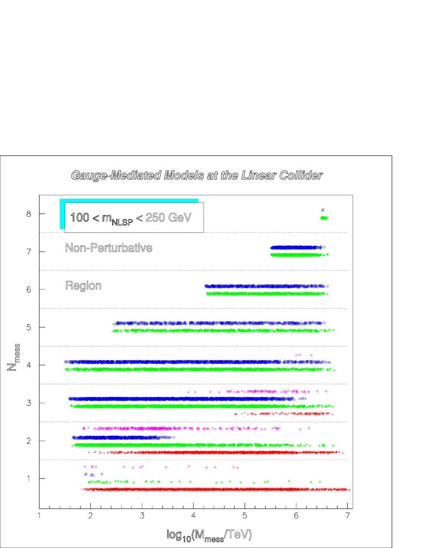
In Fig. 1, we show where in the ( plane the scenarios described above are of relevance, for a GMSB spectrum of interest for the LC. One can see that the neutralino-NLSP scenario can only occur (but does not need to) for 1, 2 or 3. For , it is also necessary to have a messenger scale as high as GeV or more. Neutralino-stau co-NLSP models exist also for , but only for very high . Stau NLSP and slepton co-NLSP models are instead possible for all allowed values of , but slepton co-NLSP models need to be lower than () GeV, if (2). Perturbativity requirements up to the GUT scale start to be effective in excluding relatively low values of for , while models with or 8 are not possible if one imposes the simple cosmology-inspired condition keV.
Within a given scenario, the specific topology of the signatures is determined by the value of . We discuss this in detail in the next section, for the specific case where a neutralino is the NLSP. We now analyse a few important characteristics of neutralino NLSP models with 100 GeV GeV in our sample.
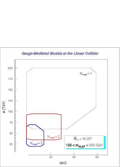
First, in Fig. 2, we show the allowed regions in the (, ) plane for such a scenario to be realized. All the neutralino NLSP models we generated fall within the regions shown in Fig. 2 for a given value of , but note that it is generally possible to construct models giving rise to different NLSP scenarios that also fall in the same regions of this plane. The regions in figure are sketched with a regular form to give a more intuitive feeling and are a bit wider than those actually populated by the relevant models in our sample. Also note that, due to the stau L–R mixing producing lower mass eigenvalues for large , it is impossible to build a neutralino NLSP model of interest here for (15), when the messenger sector is not the simplest possible one, namely (3).
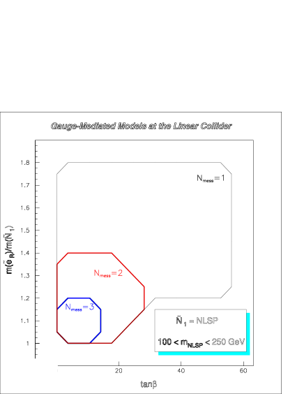
Second, it is important to determine how much heavier the other sparticles can be compared to the . This tells us what the likelihood is that once -pairs are produced as an isolated signal at the LC, one can turn other SUSY processes on by just slightly raising the available c.o.m. energy. In all neutralino-NLSP models, the next-to-NLSP particles are the -sleptons, and in particular the (which turns always out to be dominated – 85% or more – by the component). The mass is particularly relevant, since it largely determines the cross section, together with the physical composition, due to the large contribution from -channel -exchange graphs. Indeed, we will see that in GMSB models, the is dominated by the bino component, more strongly coupled to -particles, and the is always much heavier than the . The contribution from -channel -exchange graphs is hence generally negligible. In Fig. 3, we show the ratio as a function of and for different messenger multiplicity. We chose here as the independent variable mainly for visual purposes. The main information that can be extracted from Fig. 3 is that there are no neutralino-NLSP models where the is more than 1.8 (1.4, 1.2) times heavier than the for (2,3).
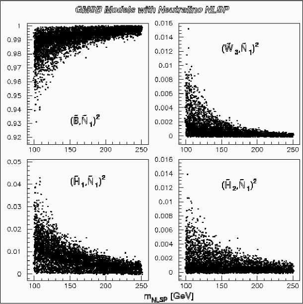
Both in connection with the production cross section and with the decay properties to be discussed in the next section, it is essential to specify the possible physical composition of the in GMSB models with neutralino NLSP. Fig. 4 shows clearly that the bino component is always well above 90%, while the wino component never reaches the 2% level. The total higgsino component in the can only rarely reach the 5% level, hence in some cases we will just neglect it in the following and assume that the is a pure gaugino. Note also that in the EW-diagonalised basis, the photino component of the NLSP is always included in the 0.60–0.85 range, while the zino component is in the 0.15–0.35 range.
The reader must be warned, however, that this is only true in the simple GMSB framework we use in this paper. Here, we chose the phenomenological approach where one just assumes the existence of the and terms at the messenger scale and determines them through EWSB conditions. As a consequence of this and the particular characteristics of the stop spectrum in GMSB, turns always out to be in neutralino GMSB models with 100 GeV GeV. Further, the relation always holds at the EW scale (here is the bino soft mass). Such a circumstance produces decoupling between the gaugino and higgsino blocks in the neutralino and chargino mass matrices and the characteristic relations approximately hold, while the heavier neutralino and chargino mass eigenvalues are always of order .
However, there are many possible sources of more complex scenarios. For instance, if one attempts to put together a radiative mechanism to generate and , one may find extra corrections to the Higgs soft (mass)2 parameters, which in turn can modify the value of , often lowering it [8, 9, 11, 22]. Further, it is possible to build coherent GMSB models that have unequal messenger multiplicity relative to the three SM gauge groups. Models in this class exist where the higgsino component of the NLSP is large, with remarkable phenomenological consequences, both for the production cross section and decay BR’s to be discussed below. Many other variations in the messenger sector are possible [23], but the associated phenomenology is beyond the scope of this paper. In the following, we will always assume that the higgsino components of the NLSP are small and possibly negligible.
We list here three reference GMSB models with neutralino NLSP in our sample that we will use in the following. We chose these particular models because they are qualitatively different for our experimental studies of Sec. 7. They cover a good spectrum of possibilities and provide a feeling of the various problems that the experimenters could face if nature had chosen GMSB and the neutralino as the NLSP.
Model # 1 features are summarised in Tab. 1, where spectrum, production cross sections at a 500 GeV LC, and other relevant details such as sparticle physical composition and dominant decay channels are given (details about the NLSP decay are deferred to the next section). The precise values reported for masses and cross sections (which include ISR and running effects), depend slightly on details of the spectrum calculation, higher-order corrections etc. They should be considered as an approximation at the level of a few percent. (Since here we are not particularly interested in the Higgs sector, we give only indicative information about it.)
| Model # 1. INPUT: 161 TeV; ; TeV; ; | |||
|---|---|---|---|
| Particle | Mass | Production @ 500 GeV LC | Comments |
| LSP | eV | indirect only | stable |
| NLSP | 100.0 GeV | fb | ; decays to |
| 136.6 GeV | fb | ; decays to | |
| , | 137.1 GeV | fb | decay to |
| 183.3 GeV | fb | ; | |
| 184.6 GeV | fb | ||
| 264.4 GeV | – – | slightly lighter | |
| , | 274.3 GeV | fb | |
| 274.5 GeV | fb | ||
| 105 GeV | fb | ||
| , , | GeV | – – | |
| , , | GeV | – – | |
| GeV | – – | ||
| GeV | – – | ||
Model # 1 is a model with a rather light spectrum, in particular the NLSP mass is right at our assumed LEP2/Tevatron bound of 100 GeV. The next-to-NLSP, the -sleptons, are in the middle of their allowed mass range for such a NLSP mass. If this GMSB scenario were to be realized, the sparticles that could be produced with appreciable cross section at a 500 GeV LC would be gauginos, -sleptons and -selectron (in association with ). The total GMSB signal would be in this case quite “generous.” Heavy interacting sparticles are definitely out of reach, even for a possible second phase of LC operations with c.o.m. energy at or slightly above 1 TeV. These large mass splittings are a well-known characteristics of GMSB models (cfr. e.g. Refs. [3, 24]) and are due to the fact that gaugino and scalar masses are proportional to the relevant gauge couplings. (The light Higgs is close to the edge of detectability at LEP2/Tevatron, depending on fine details and higher-order corrections that we do not take into account. In any case, models with a slightly heavier and no significant differences in the other sectors can easily be constructed with small changes to the input parameters. The rest of the Higgs sector is very heavy.) Notice that such a model would not be expected to produce a large signal at the LHC, due to the heaviness of gluino and squarks, hence a careful search and study at the LC would be most likely necessary, if not for initial SUSY discovery, then at least for a confirmation and for determining with good accuracy the source of the anomalous signal and the underlying SUSY-model parameters.
| Model # 2. INPUT: 309 TeV; ; TeV; ; | |||
|---|---|---|---|
| Particle | Mass | Production @ 500 GeV LC | Comments |
| LSP | eV | indirect only | stable |
| NLSP | 200.0 GeV | fb | ; decays to |
| 115 GeV | fb | ||
| 256.4 GeV | – – | ; decays to | |
| , | 256.8 GeV | – – | decay to |
| 374.1 GeV | – – | ; | |
| 374.4 GeV | – – | ||
| 511.5 GeV | – – | slightly lighter | |
| , | 516.7 GeV | – – | |
| 516.7 GeV | – – | ||
| , , | GeV | – – | |
| , , | GeV | – – | |
| GeV | – – | ||
| GeV | – – | ||
Model # 2 (see Tab. 2) is much more of an “avaricious” model, with a 200 GeV NLSP mass. It is obtained from Model # 1 by just raising the input value of , leaving the ratio and the other parameters untouched. The only GMSB signal present at a 500 GeV LC would be NLSP pair production in this case. Note that changing the mass with respect to Model # 1 does not only result in a drastic reduction of the cross section for production, but also in an important change in the decay BR’s, as described in detailed in Sec. 3. As a consequence, even focussing on production only, this model would produce a considerably different signal at the LC compared to Model # 1, both quantitatively and qualitatively. In this case, gluino and squarks are very heavy, possibly close to a reasonable bound from naturalness arguments and the GMSB signal at the LHC would be rather scarce.
| Model # 3. INPUT: 110 TeV; ; TeV; ; | |||
|---|---|---|---|
| Particle | Mass | Production @ 500 GeV LC | Comments |
| LSP | eV | indirect only | stable |
| NLSP | 165.0 GeV | fb | ; decays to |
| 171.5 GeV | fb | ; decays to | |
| , | 171.8 GeV | fb | decay to |
| 315.0 GeV | fb | ||
| 105 GeV | fb | ||
| 315.1 GeV | – – | ; | |
| 342.5 GeV | – – | slightly lighter | |
| , | 349.8 GeV | – – | |
| 349.8 GeV | – – | ||
| , , | GeV | – – | |
| , , | GeV | – – | |
| GeV | – – | ||
| GeV | – – | ||
Model # 3 (see Tab. 3) is a special model presenting some unusual and challenging characteristics. First of all, the -slepton masses are very close to the neutralino NLSP mass of 165 GeV. (Note that when the difference between the mass and the NLSP mass approaches the tau mass, one falls in the neutralino-stau co-NLSP scenario that we are not treating here.) As we will see, this poses the problem of separating the various GMSB signals from each other at the LC in order to perform specific measurements. Another experimental challenge follows from the fact that the relatively low minimum gravitino mass combined with a quite large mass makes it possible for the neutralino to decay very close to the interaction region at the LC (see Sec. 3) in this case.
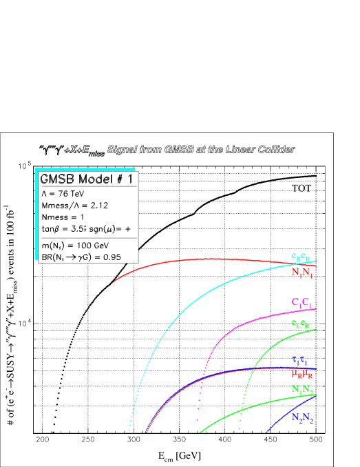
In Fig. 5, we plot the cross-section for the various SUSY production processes as a function of in the range of interest for a 500 GeV LC, for Model # 1. Actually, Fig. 5 contains some more information, since the normalisation of the y axis takes into account the inclusive nature of the GMSB signal and the typical luminosities of the LC. As we will see in Sec. 3, for all neutralino NLSP models is the dominant NLSP decay channel, with BR’s always greater than about 85%. (For Model # 1 this is actually 95%.) As a consequence, each time a sparticle pair is produced, there is a large probability of getting a final state with 2 photons, some other particle resulting from cascade decays and large missing energy. In Fig. 5, the quotation marks for mean that (one of) the photons might escape detection if the lifetime is very large (cfr. Sec. 3). The number of “”“” + X + events is normalised to an integrated luminosity of 100 fb-1, which is a typical value for a few-month run at the LC (cfr. Sec. 4). Notice here that for the case of Model # 1, running at c.o.m. energies of order 270 GeV would still allow for order 20,000 GMSB events, while selecting pure events only. This circumstance will be exploited for our experimental studies in Sec. 7. We will also use Fig. 5 as a basis for the study of Sec. 5.
3 Neutralino NLSP Decays
In this section, we analyse the properties of the NLSP decay in GMSB models, with focus on the case where NLSP.
In Ref. [10], all the formulas for 2-body decays involving the gravitino can be found, in the limit where the gravitino interactions can be approximated by those of the goldstino and its mass can be kinematically neglected, which is always the case in GMSB at collider energies. For a generic decay , where S is a SM particle and its MSSM superpartner, one has for the corresponding width,
| (4) |
where the gravitino mass is given by (1), is the relativistic factor if is a vector or scalar boson. If is a massless fermion, . is a constant depending on the , spin and possibly a mixing matrix element. For example, if is a SM lepton or quark and a slepton or squark, then simply .
We are here interested in the case, since in our neutralino NLSP models the only particle that can undergo a 2-body decay to a gravitino with a non-negligible width is the lightest neutralino. The relevant expressions for can be found in Tab. 4, where we use the notation of Ref. [21] for the neutralino mixing matrix and is the mixing angle in the MSSM neutral Higgs sector.
| Decay Channel | where | |
|---|---|---|
Due to the absence of the kinematic suppression and the physical composition in the models of interest here (cfr. Fig. 4), the decay is always dominated by the photon channel. However, in the context of this paper where GeV and fine details of the neutralino decay will be used in the following, it is important to note that the BR for decaying to a can be sizeable and also to address the problem of the 3-body decay channels , where is a SM lepton or quark [9].

The Feynman diagrams contributing to the 3-body processes are shown in Fig. 6. An analytical formula for the sum over final-state SM-fermions of the total widths for these decays via real or virtual boson exchange has appeared in Ref. [9]. However, that summed formula could not take into account Diags. 6–9 where a - or -sfermion is exchanged, which are a-priori not less relevant than Diags. 2–5, where other heavy intermediate particles are involved. Also, in Ref. [9] the virtual photon contribution (Diagr. 1) was calculated including an overall detector-dependent cutoff on the fermion pair invariant mass, chosen to be of order 1 GeV. In the context of this paper, however, we have at our disposal a full detector simulator (cfr. Sec. 6) and we will be interested in the individual BR’s for each pair (cfr. Sec. 7). Also, the kinematical distributions of these decays are relevant to our following studies. In the rest of the paper, we will often use the name “neutralino charged decays” when referring to the channels and in particular to the case where the subsequent final state includes either a charged lepton or a charged “stable” hadron.
To account for these channels, we proceeded as follows. Using the general lagrangian for the goldstino interactions with matter without assuming on-shell conditions (cfr., e.g., Refs. [3, 10]), we input all the relevant vertices111For some of our gravitino vertices and using the goldstino lagrangian as an input, we checked that there is agreement with the output of LanHEP 1.5.06 [25] involving the gravitino in CompHEP 3.3.18 [26] in a limit suitable for collider physics. For the other vertices involving MSSM particles, we used the home-made lagrangian222For the relevant MSSM vertices and in the relevant limit, we checked that there is numerical agreement with our results when using the CompHEP 3.3-compatible MSSM lagrangian of Ref. [27] instead. that was first checked against analytical calculations and then used for numerical evaluations in the work of Ref. [20]
We named the resulting software Gravi-CompHEP [19]. Using Gravi-CompHEP, we found that the contribution to the total width from virtual photons is in very good numerical agreement (for the electron and muon case up to 4 digits) with the analytical formula [28], valid to lowest order in ,
| (5) |
where is the final fermion electric charge in units of , for leptons (quarks) and the cutoff is naturally provided by the mass. Note that, e.g. for a 100 GeV neutralino mass as in Model # 1, Eq. (5) gives for the case of electrons in the final state numbers about twice (five times) as large as for the case of muons (taus). For hadronic final states, a realistic evaluation must take hadronization effects and higher-order corrections into account. However, since hadrons will not be our main focus in the analyses of Sec. 7 and we will be most interested in the BR’s for the leptonic channels, we chose a reasonable approximation using a rough cutoff for the invariant mass of the final fermion pair at MeV for light quarks and Eq. (5) for heavy quarks.
The contribution from -exchange to (Diagr. 2) is obtained from Eq. (4) by replacing
where and are kinematical factors taking finite -width effects into account333Analytical expressions can be found in Refs. [9, 10]. In our model sample for the LC, one finds that as long as GeV the on-shell approximation is accurate at the level of 10% or better. For lighter neutralinos, the full calculation is required, since e.g. for GeV one has and , whereas , and the on-shell approximation underestimates the Diagr. 2 contribution by a factor 2.5–3. On the other hand, for models with GeV in our sample, the -exchange contribution is always of the virtual photon contribution, e.g. for the case.
The interference between the - and -exchange diagrams turns out to be always small, generally at the level of a few % or less of the pure Diagr. 1 contribution (cfr. also Ref. [9]).
Diagr. 3 is always negligible for the models of our interest here. Indeed, one has both a dynamical suppression due to the lack of higgsino components in the (cfr. Fig. 4) and a kinematical suppression, for GeV (in this range, always in our model sample and the on-shell approximation applies). Taking off-shell effects into account for GeV (the formulas are similar to those for the case described above) does not help either, since the width is typically very small in the MSSM. Also, Diagr. 3 contributes to the channels with heavy fermions in the final state only, which have typically lower BR’s. Diags. 4 and 5 are even more strongly suppressed, because the masses of the CP-odd and heavy CP-even Higgses only rarely drop below 300 GeV in our model sample. Interferences involving Diags. 3–5 are basically zero. In the rest of this section, we will often assume for simplicity that the is pure bino; this makes all the contributions from Diags. 3–5 zero and is justified by Fig. 4.
Finally, as far as Diags. 6–9 are concerned, the exchanged is necessarily heavier than the initial by definition of neutralino NLSP model. For the case of hadronic final states, these diagrams do not count, since the squarks are too heavy in our models. However, it turns out that limited to the case of exchange, the contribution to the width is often non-negligible and at the level of several to 10% of the total, especially for those models where is close to 1 and for the case of heavier leptons in the final state where Diagr. 1 is less dominant. This is again due to the relatively large coupling and the fact that the can never be much heavier than the NLSP (cfr. Fig. 3). Diags. 6–7 are always negligible, even in the leptonic case, due to the relative heaviness of the -sleptons.
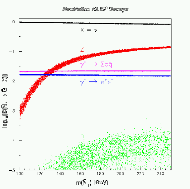
In Fig. 7, we give a general idea of the behaviour of the BR’s for the main neutralino NLSP decay channels as a function of for all the models in our sample of interest for the LC. From top to bottom, we show the BR’s for the dominant two-body channel to a photon, the two-body channel to a including off-shell effects (so that the contribution from Diagr. 2 to 3-body channels can be readily extracted by multiplying by the appropriate BR), the hadronic and 3-body channels from Diagr. 1. For comparison, we also report our results for the BR of the 2-body decay in the on-shell approximation. The logarithmic scale does not allow inspection of fine effects. However, it is evident that the channel can be important with BR’s up to about 15% for heavy neutralinos, while the main 3-body channels via virtual photon are always relevant with BR’s at the level of a few %. The Higgs channel has always BR’s less than 0.1%. Note also that, due to the homogeneous physical composition of the in our sample, the important BR’s are basically dependent only on the neutralino mass.
Fig. 8 is a scatter plot for our model sample showing in detail the BR’s for all the
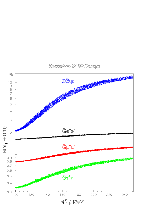
3-body decay channels (excluding ) as a function of the neutralino mass. From top to bottom, hadronic + , , and final states are calculated including all contributions from Diags. 1–9 in Fig. 6. The BR’s for all 3-body channels all increase for heavier neutralinos. The hadronic channel occurs about 2% to 15% of the times, the electron channel 1%–1.5%, the muon channel 0.8%–1.1%, the tau channel 0.3%–0.7%. Again, fixing the mass basically determines these BR’s, with some more uncertainty for the hadron and channels that receive relatively larger contributions from -exchange.

In spite of the fact that the BR for the leptonic 3-body channels is often quite low, due to the large integrated luminosity that might be available at a LC, the possible number of events featuring a (displaced) pair is still large in most cases. In Fig. 9, we show scatter plots for our neutralino NLSP model sample referring to inclusive GMSB signals at a GeV LC as functions of the neutralino mass. We refer to a nominal 100 fb-1 run and sum over all SUSY production processes. In Fig. 9(a) we report the number of events including two (displaced) photons and missing energy coming from two long-lived neutralino decays. In Fig. 9(b), we consider all events including at least a displaced pair and missing energy. In the models we are interested in, one gets at least 100 such events if GeV, and up to about 10,000 events for lighter neutralinos. Notice that the meaning of “displaced” here is that the tagged particles are produced at some distance from the interaction region, where the distance depends on the neutralino lifetime and the specific processes considered. In some cases, the displacement might be so large that the particles are actually produced outside the detector, as we will see in the following.
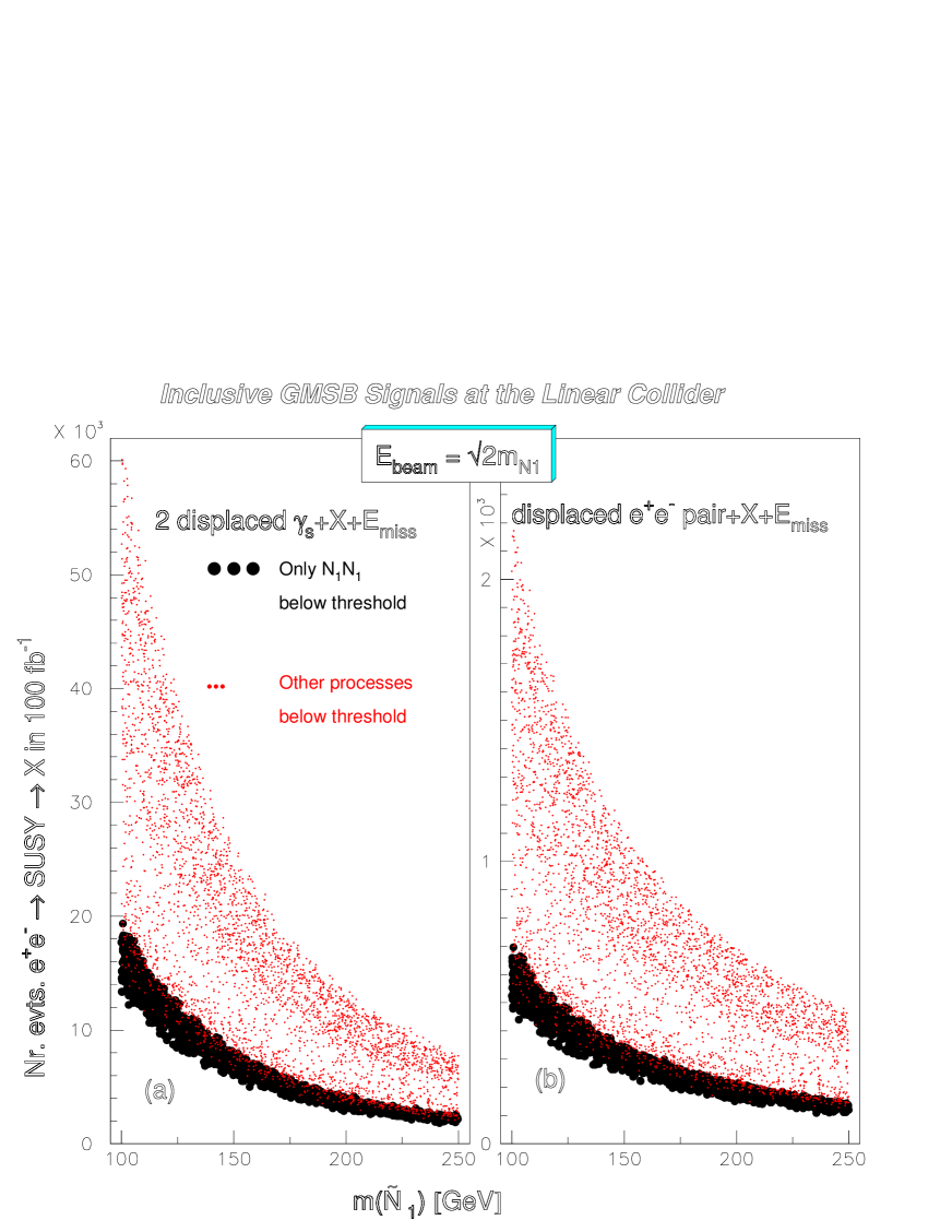
In Sec. 7, we will see that it is sometimes useful to run a LC at a c.o.m. energy not far from the threshold to isolate the signal from neutralino pair production. To give a feeling about this problem, in Fig. 10 we show a scatter plot similar to Fig. 9, but for . The big black dots refer to models for which only pairs can indeed be produced at such an energy, while small grey dots are for models where other processes (typically pair production of -sleptons) are also below threshold. Note that the number of events including a displaced pair is always larger than about 100 for an integrated luminosity of 100 fb-1. The BR’s for all the main decay channels for the three reference models introduced in Sec. 2 are shown in Tab. 5 and will be referred to in the analyses of Sec. 7.
| Decay Channel | BR in Model # 1 | BR in Model # 2 | BR in Model # 3 |
|---|---|---|---|
| 0.9507 | 0.8395 | 0.8913 | |
| 0.0003 | 0.1115 | 0.0585 | |
| 0.0164 | 0.0191 | 0.0179 | |
| 0.0079 | 0.0117 | 0.0101 | |
| 0.0034 | 0.0076 | 0.0059 | |
| 0.0213 | 0.0999 | 0.0631 | |
| 0.0002 | 0.0223 | 0.0117 | |
| – – |
In Sec. 7, we will heavily use the characteristics of the three-body decays of the neutralino, including their kinematical distributions. Using Gravi-CompHEP, we calculated such distributions for our reference models and we show here our results. We then implemented numerically the corresponding differential widths into our event generator to perform the Monte Carlo simulation.


In Fig. 11, the normalised invariant mass distribution for all the leptonic channels is plotted. The stars, circles, crosses are the central points of our results for the electron, muon, tau cases respectively in Model # 1 (a) and Model # 2 (b). The horizontal bars show the binning we used, while the errors coming from numerical phase space integration on the distributions are too small to be visible in logarithmic scale in most cases. Note that the distributions are sharply peaked for low invariant masses close to and this is more and more true for lighter leptons. As a consequence, e.g. the pairs coming from production at the LC and subsequent three-body decay of (one of) the neutralinos tend to be generated with small separation angles, which introduces some experimental challenges (cfr. Sec. 7). In Fig. 11(b), the peak corresponding to the -exchange contribution is also evident. To allow a better inspection of the scaling properties of the distributions with and , we used here the (very good) approximation for both models, so to keep the physical composition constant when going from Model # 1 to Model # 2. For the case of Model # 1, we included Diag. 1 only of Fig. 6, since the other contributions would hardly be visible in the plot anyway.

Limited to the case of Model # 1, in Fig. 12, we show some relevant angular distributions for the decay, the three-body channel we will be most interested in. The circles refer to the normalised distribution, where is the angle between the electron and the positron momenta in the decaying rest frame. As expected, the and the prefer to proceed along the same direction, due to the dominance of the virtual photon contribution. The stars correspond to the normalised distribution, where is the angle between the electron (or positron) and the gravitino momenta in the rest frame. The pair is produced in the direction opposite to the in the great majority of cases. The squares refer to the normalised distribution, where is the angle between the electron (or positron) momentum and the direction of the boost of the system with respect to the rest frame, calculated in the rest frame. In our case, this is basically the angle between the electron (or positron) and the virtual photon momenta and the almost constant behaviour is then expected. Finally, the crosses show the normalised distribution, where is defined as above and refers to the system instead of the one. The general behaviour of these angular distributions is better understood in the light of the fact that the two-body decay is isotropic. Some instability of our results due to numerical phase space integration is visible, but it is well within the shown vertical error bars.


In Fig. 13, we show the normalised energy distributions for the decay in Model # 1 (a) and Model # 2 (b). The stars refer to the electron (or positron) energy, while the circles are for the gravitino energy, in the decaying rest frame. For the case of Model # 1, the tends to take half of the available energy, while the electron and positron share the rest with an almost uniform distribution between and about . Model # 2 features evident effects of the -exchange contribution that add to a behaviour similar to the one for Model # 1 coming from the still dominant virtual photon contribution. Again, in order to allow a cleaner comparison between the two models, we used here the bino approximation. Note that both the scales on the x and y axes in Fig. 13 are interrupted for display convenience.
After having inspected the various possible decay channels, we turn now to the discussion of the total width and the lifetime of the neutralino. As anticipated above, this determines the topology of the signatures of neutralino GMSB models at colliders. A single neutralino produced with energy will decay before travelling a distance with a probability given by
| (6) | |||||
| (7) |
is the “average” decay length and is the kinematical factor . Note that for pairs directly produced at the LC with GeV, (0.75) if (200) GeV.
Using Eqs. (1), (4), and (5), the neutralino lifetime can be conveniently expressed in the suggestive form,
| (8) | |||||
which stresses the scaling properties with the 5th inverse power of the neutralino mass and the 4th power of the fundamental SSB scale. is a number of order unity that can be well approximated by when the two-body channel widely dominates, as e.g. in Model # 1, or by simple expressions in most cases. In general, however, it is a complicated function of the neutralino composition, the GMSB model spectrum etc., when the full contributions to the three-body channels are taken into account.
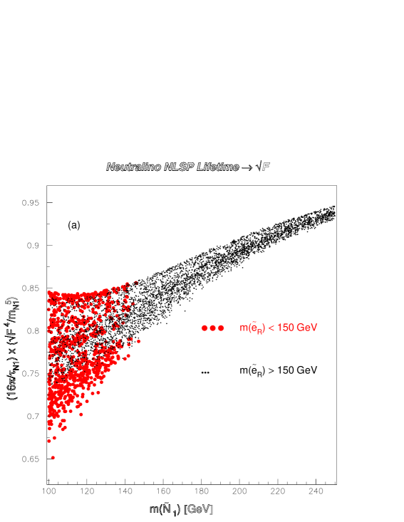
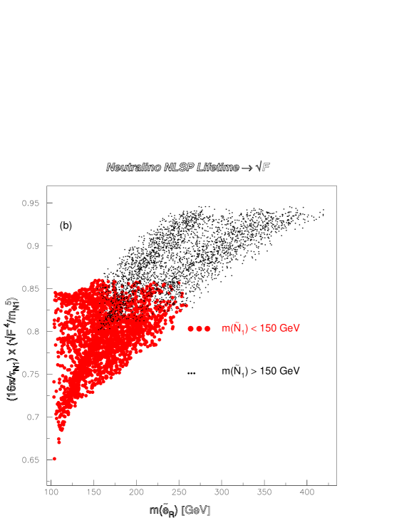
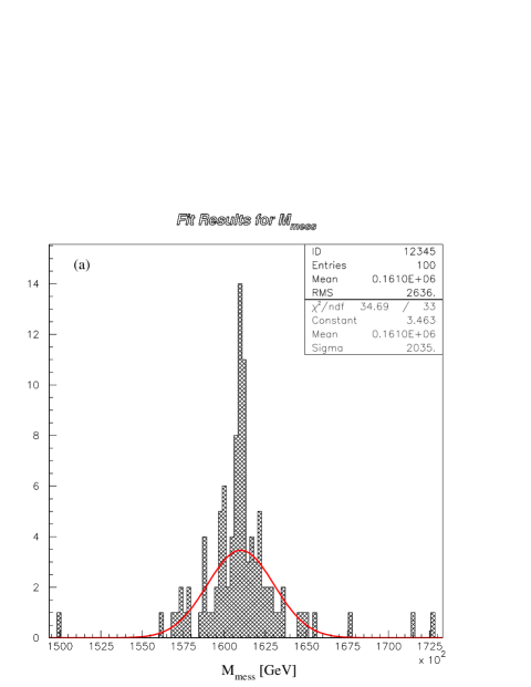
Once the neutralino mass and lifetime are measured (cfr. Sec. 7), one can get striking information on from Eq. (8). The uncertainty is then only due to the factor . If the BR’s for the various decay channels are also measured with good precision, or the neutralino composition and the (light) GMSB spectrum is extracted by measuring other observables (production cross sections, distributions), the fundamental SUSY breaking scale can be determined precisely. However, it is remarkable that even without collecting additional information, the knowledge of and is sufficient to constrain the value of in a narrow range, based on the well defined characteristics of GMSB models. In Fig. 14, we report scatter plots of our neutralino NLSP model sample for the LC showing in Eq. (8) as a function of the neutralino mass (a) and the right selectron mass (b). To stress the existence of some correlation between and the right selectron mass for models with a fixed light neutralino mass, in Fig. 14(a), the big grey (small black) dots refer to models where 102 (150) 150 (430) GeV. This can be compared to Fig. 14(b), where big grey (small black) dots correspond to models with GeV. From this, one can e.g. infer that if GeV and the neutralino lifetime is measured to be about 1 cm, then TeV. If, in addition, is measured to be heavier than about 150 GeV (for instance, from threshold scanning, see Sec. 5, or using its impact on the cross section), then the allowed range is further reduced to 370–385 TeV. For a 200 GeV neutralino, a 1 cm lifetime gives TeV.
To summarise, we note that in the absence of further information, the theoretical error on determining from given values of mass and lifetime amounts to about 3% in the worst case, helped by the 4th power dependence in Eq. (8).
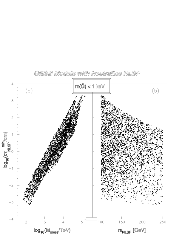
It is of primary importance for collider phenomenology to assess the range of variation for . As anticipated in Sec. 2, it is possible to use a lower limit from theory on , while significant upper limits can only come from weak cosmological arguments suggesting keV. The lower limit defines a minimum value for the neutralino lifetime as well as for the gravitino mass on a GMSB model-by-model basis. In Fig. 15, we plot this limit as a function of (a) and (b) for our model sample of interest for the LC. In this plot, we also use the cosmological upper limit on , in the sense that those models where keV are not plotted. As a result, one can see that the neutralino lifetime can be anywhere between about 5 microns and about 25 metres (or more if no cosmological arguments are used). Models with a high messenger scale produce longer neutralino lifetimes. For instance, if TeV, then is always larger than about 1 cm. Also note that shorter lifetimes are obtained for heavier neutralinos. A 100 GeV neutralino will always live more than about 15 microns. On the other hand, a 250 GeV neutralino will tend to decay well within a typical detector size, with lifetimes always smaller than about 20 cm, if cosmological arguments are used.
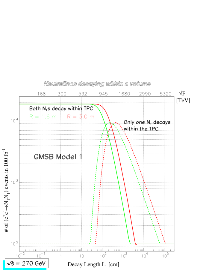
When SUSY pairs are produced in a neutralino NLSP scenario, the resulting final states always include two neutralinos, which in turn decay to a gravitino + X. The probabilities of both, one or zero neutralinos decaying within a given volume of the detector depend on the neutralino’s decay length of Eq. (7), which in turn depends on the specific SUSY process, model and collider c.o.m. energy one is considering. If we define a spherical volume of radius , then the probabilities associated with these circumstances are of course given by , , and . In Fig. 16, we show how many events are expected with two (solid line) or one (dashed line) neutralino decays as a function of (or ) for the case of direct neutralino-pair production in Model # 1. We show curves for two reference spheres with a radius of 160 and 300 cm (we will see in Sec. 6 that the outer cylinder of a typical proposed TPC for a LC detector is included between such two spheres). Our numbers refer to a 100 fb-1 run at the LC with GeV, where only pairs can be produced with a cross section of 188 fb. This choice of parameters will be of relevance for the studies to be presented in Sec. 7. Note that for neutralino decay lengths as large as 1 km (and larger than 5000 TeV), there still are about 100 events where one neutralino decays within the reference volume. We warn however that this is only true if a sum over all possible final states coming from neutralino decays is performed and no angular or other detector acceptance cuts are taken into account. Based on this, a refined statistical study based on a realistic cylindrical detector and experimental framework for the LC is performed in Sec. 7.7.
4 The Linear Collider and the TESLA Project
The LHC will explore the next high energy frontier and can be expected to be among the prime sources of new physics discoveries into the next decade and beyond. However, ongoing studies of the physics potential of a LC operating at c.o.m. energies ranging up to 500 GeV, or higher (1–2 TeV), are revealing many complementary measurements that could be made at such a machine on a similar timescale to that of the LHC. Additional options available at a LC are a considerable electron (and possibly also positron) polarisation, and options, as well as the potential for collisions, making a LC a very flexible and relevant facility, with particular application to detailed studies of new physics signals.
Several linear collider designs are presently under discussion [29] and much of the discussion in this paper is applicable to any machine. However, in order to relate our study to a specific case, we explore the machine parameters of the high-luminosity TESLA option. The TESLA machine proposal is described in some detail in vol. 2 of the ECFA/DESY “Conceptual Design Report” (CDR) [30]. The most recent proposals involve two phases of operation; an earlier phase operating at GeV or less and a later phase operating at GeV or less, with luminosities of cm-2s-1 and cm-2s-1 respectively [31]. In this study, we mostly limit ourselves to the first phase foreseen for such a collider, with varying between approximately 200 and 500 GeV. In most cases, we will consider results that can be obtained after collecting an integrated luminosity of 200 fb-1, corresponding to approximately one year of running at TESLA and to a few years of running if parameters proposed for other linear collider options (such as JLC or NLC [29]) are used.
We should stress that one of the highly desirable features of a LC is the ability to tune the c.o.m. energy to explore thresholds with precision. In this way, specific signals, e.g. from SUSY, can be enhanced from among others, unless the production thresholds are too closely degenerate. For instance, we use this property below for our GMSB models # 1–2 to isolate the neutralino pair production process for individual study. In addition, the energy can be tuned to alter appreciably the Lorentz () factors of the produced neutralinos and hence extend the range of NLSP lifetime measurements. Neither of these options will be available at the LHC.
A further advantage to this study of a LC over the LHC is the fact that the effective c.o.m. energy is known precisely, up to effects of initial state radiation (ISR) and beamstrahlung. The values of due to beamstrahlung are estimated to be 2.8% and 4.7% for the first and second phase of TESLA respectively [31]. For the processes we study in this paper, it is of prime importance to know the energy of the pair-produced neutralinos in order to be able to reconstruct the neutralino decay length, as described further in Sec. 7. We wish to stress here the complementary nature of the LC with respect to the LHC and we envision the pleasing scenario where the LHC provides a wealth of interesting data, which is subsequently investigated at the LC with high precision. This may indeed be necessary in order to distinguish conclusively between GMSB and other possible SUSY realizations (e.g., no-scale SUGRA models) and to measure the fundamental parameters with the precision needed to extract striking conclusions concerning physics at the messenger and higher scales. Because of this, the present LC detector design proposals should be flexible enough to benefit at a late stage from LHC new physics data. Our study attempts to address this issue and we will further comment on this in Sec. 8. Moreover, as we already pointed out in Sec. 2, GMSB models often feature very heavy strongly interacting sparticles, which could not provide a large signal at the LHC. In this case, the rôle of the LC in determining the origin of the new physics signal would be even more important.
5 Disentangling a Signal from GMSB at the Linear Collider
In this section, we provide an example of how it might be possible to extract a good amount of information about the parameter values of the underlying model from the observation of an abundant GMSB signal at the LC and a simple threshold scannning technique. Let’s assume that Nature has chosen GMSB and that Model # 1 is realized. Let’s also assume for simplicity that is not too large, so that (most of) the produced NLSP’s decay within the detector. If this is the case, just a few weeks of LC running at some initial c.o.m. energy between 200 and 500 GeV would be enough to recognize the presence of an evident GMSB-like scenario. Indeed, a copious number of events with two ’s and large missing energy would show up, due to the inclusive characteristics of the GMSB signal. Further, we will see in Sec. 7 that in most cases it will be possible to show that these photons do not point to the interaction region, and hence are likely to come from a delayed neutralino decay, since the SM background is essentially zero. (Of course, at least in the case of Model # 1, it is very reasonable that at the moment of starting the LC operations clear indications for GMSB would have already come from the LHC.) Among the two-photon events, there will be many coming from production featuring no other particles and, if GeV, many others including (soft) pairs from selectron-pair production as well. If the c.o.m. energy is even larger, then more complex events, many with hadronic activity, would also appear from, e.g., production.
A feeling of the situation can be obtained from inspection of Fig. 5. In Sec. 4, we stressed the importance of the ability of a LC of tuning the c.o.m. energy to explore thresholds with precision. First, one could vary in big steps and just inclusively count two-photon events to get the rough location of the thresholds for the various SUSY-production processes (cfr. thick line labeled “TOT” in Fig. 5). Then, one could focus on the individual thresholds, observe more exclusive characteristics of the signal (for instance, production gives events only, with well-defined lepton energy spectra, since -sleptons will always decay to , and so forth), and vary in finer steps to get a precise value of the sparticle masses involved in the corresponding production process. For the case of a GMSB model like Model # 1 where about 10 thresholds are present below GeV, it seems reasonable to assume that a 200 fb-1 run (less than 1 year, based on the TESLA expected performance) would allow extraction of the light masses with errors at the level of fractions of a GeV. Of course, the fine details depend on the slope and the magnitude in the vicinity of the thresholds of the curves for the various individual cross-sections as functions of (cfr. Fig. 5). For instance, in absence of important -channel contributions, one would expect a steeper behaviour for gaugino-pair (fermion) production compared to for slepton-pair (scalar) production, so that gaugino masses could generally be determined with higher precision [32]. On the other hand, in our case the -channel contributions are important and, in addition, one can always imagine to spend more machine time running close to the “harder” thresholds and also use other observables (e.g. distributions) to get additional information on the spectrum.
Our intent here is not to simulate fully such a complex study, but to evaluate what could be the sensitivity in determining the GMSB parameters from the knowledge of the light spectrum that could come from a roughly uniform threshold-scanning. Based on Model # 1 and a total of 200 fb-1 collected between 200 and 500 GeV c.o.m. energies, we estimated the following approximate precisions for the sparticle masses:
| (9) | |||||
The assumption on is based on the fact that many events would be observed at the LC if Model # 1 is realized and many other Higgs events would have already seen and studied at the LHC444 Here, we assume that the theoretical error on determining the lightest Higgs mass from any SUSY-model input parameters, currently at the level of at least a few GeV [33] will be reduced by that time by more detailed calculations. Similarly, we imagine that the theoretical error on the sparticle masses will also be brought at a level comparable to the numbers quoted above.
Also, in Sec. 7.2, we will see that a measurement of the mass with a precision at the level of a few tenths GeV can be easily achieved by looking at the energy spectrum from decays.
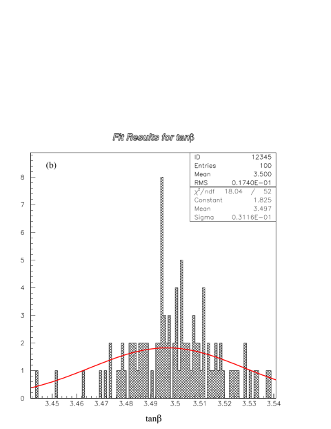
We used a home-made computer program called MinuSUSY [19], interfaced to SUSYFIRE and Minuit [34], to perform fits to SUSY-model basic parameters starting from information on the sparticle spectrum555MinuSUSY does not take higher-order corrections to the sparticle masses into account, but these can typically be reabsorbed in a redefinition of the basic model parameters and a shift of the starting values needed to generate a given spectrum. For our purpose here, however, the precise values of the SUSY parameters are not the point, since we are only interested in evaluating the level of sensitivity one could reach by using these techniques. We believe our indications in this respect to be found below are still valid without taking fine effects into account.. The program works both with (m)GMSB and (m)SUGRA models and in “global” or “local” mode. The “global” mode is intended to determine which class of SUSY models and which approximate values of the basic parameters best recover the input spectrum. We used this run mode starting from the light spectrum of Model # 1 (cfr. Tab. 1) and found that indeed there is no mSUGRA model that can reasonably fit it. Such a spectrum could be recovered with good precision only by releasing one or more of the unification assumptions at the GUT scale. In contrast to mSUGRA, the minimal GMSB framework allowed us to single out a successful region of the parameter space including Model # 1. Once a rough knowledge of the basic parameter values is obtained, it is possible to run MinuSUSY in “local” mode around these values and get optimised values and errors on them based on the input errors on the sparticle masses. Basically, one simulates a large number of possible sets of mass measurements using a gaussian distribution for the masses around the central values that one would get from the chosen underlying SUSY model. Starting from the errors on the masses for Model # 1 quoted in Eq. (9), we simulated 100 sets of measurements of the light sparticle spectrum. Our results for the 100 subsequent reconstructions of the GMSB parameter set performed with MinuSUSY are summarized in Figs. 17, 18, for and , and , respectively. Here we did not require to be an integer and considered it as a real variable to perform the fits. (Notice that non-integer values of are possible in some non-minimal classes of GMSB models, cfr. e.g. Ref. [23].) A gaussian (+ constant) fit to the distributions gives the results shown in Tab. 6. As for the sign of , we found that the best fits are obtained for , as expected.
| Parameter | Fitted value |
|---|---|
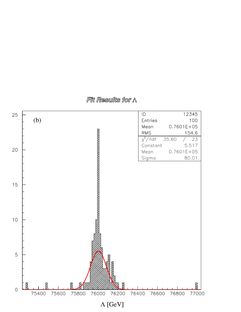
| () TeV | |
| () TeV | |
Tab. 6 indicates that it seems possible to determine and with a precision of about 1 part in and with 1 part in , by just using threshold scanning and sparticle masses as observables and running for less than 1 year at a LC with GeV. Of course, to achieve such an impressive goal, it is crucial that one can count on the high-luminosity, such as the option proposed for TESLA. The only parameter that could not be determined at a level of 1% or better is , but this is well understandable since the sparticle masses depend only logarithmically on it. Better precision could well be reached if other observables (total cross sections, distributions, branching ratios etc.) were added to the global fits. On the other hand, it must be said that Model # 1 is a particularly “easy” model, in the sense that it yields a light spectrum and the various thresholds are well separated. It would be much more difficult if the scenario of Model # 2 (for which LC energies well above 500 GeV would be needed to extract the GMSB parameters) or Model # 3 (with many sparticles almost degenerate) were realized.

6 Event and Detector Simulation
To generate GMSB events we used a modified version of SUSYGEN 2.20/03 [35], where the 3-body neutralino decays were added and the corresponding kinematical distributions were input numerically, according to the discussion of Sec. 3 and the results obtained with Gravi-CompHEP, for our reference Models # 1–3. For each GMSB model, the relevant input cards to SUSYGEN were calculated with SUSYFIRE, keeping (and hence the lifetime) as a free parameter, subject to the bounds discussed in Secs. 1 and 3. The generated events were then passed to our detector simulation software, BRAHMS [36]. This is a GEANT 3.21 [37] code including material and tracking detectors, as motivated by the ECFA/DESY CDR [30]. The relevant detector components are simulated as follows.
The beampipe is taken as a tube of beryllium of radius 1.0 cm and thickness , where is the radiation length. Five layers of vertex detectors (VXD), each of thickness and point resolution of 3.5 m are located at radial positions of 1.2, 2.4, 3.6, 4.8 and 6.0 cm, with respective half -lengths of 2.5, 5.0, 7.5, 10.0 and 12.5 cm.
We include an intermediate tracking chamber (ITC) as material with a total of and dimensions 12 cm cm and cm, but we do not consider this detector for the track fit. In the forward and rear directions, we include a forward tracking detector (FTD) made of disks of silicon strip detectors each of thickness 300 m at -positions of 40, 50, 120, 140 and 160 cm, with outer radii of 10, 10, 30, 30, 30 cm respectively and inner radii of 2.5, 2.5, 10.1, 11.7, 13.3 cm. All elements have resolution of 25 m.
We use a time projection chamber (TPC) as central tracker with inner active radius of 38.6 cm, outer active radius of 162.6 cm and active longitudinal half-length of 250 cm. The active volume is filled with gas (which we take to be argon) and provides a maximum of 118 hit points along a track, each with point resolution of 160 m in and 0.1 cm in . The inner wall to the TPC consists of a total of of aluminium. This is an important source of conversions which we discuss further in our analysis below.
For the calorimeter part of our simulator, we use an electromagnetic calorimeter (ECAL) and assume simple gaussian smearing with resolutions motivated by those in the CDR and given in Tab. 7.
| Angular Coverage | |
|---|---|
| Barrel - Dimensions (cm) | |
| Endcap -Dimensions (cm) | |
| Energy Resolution (%) | |
| Spatial Resolution (cm) | |
| Angular Pointing Resolution (mrad) | |
| Time Resolution (ns) |
In addition to the detector resolutions, there is an additional uncertainty in the position of the i.p. due to the beam spot size. In the following, we take the beam spot dimensions as given by the TESLA machine design parameters at 500 GeV c.o.m. energy [31] and thus apply gaussian smearing to the production vertex of the neutralinos with nm , nm and m.
7 Measuring the NLSP Properties and the
Fundamental SUSY Breaking Scale at the LC
In this section, we focus on practical methods to measure the NLSP properties and, in particular, its mass and lifetime. As discussed in Sec. 3, in GMSB (or in more general LESB) models, the NLSP lifetime can be macroscopic and this opens a very important window for inspecting SUSY breaking physics, which is not available in HESB models, like mSUGRA. Indeed, as Eq. (8) shows, measuring and determines the fundamental scale of SUSY breaking up to the factor (cfr. Fig. 14), that can also be measured in principle. We refer to the specific case of neutralino NLSP scenarios and, in particular, to the typical Models # 1–3 discussed in Sec. 2.
7.1 Overview of Experimental Techniques
In the following, we will first describe several techniques that we propose for performing such measurements. Depending on the lifetime, these methods involve (and test) different parts of the detector, requiring high and somewhat unusual performances. Hence, this study could be an important benchmark in the process of designing a LC detector and the related simulation software and should not only be seen as limited to SUSY searches.
We assume here that at least one SUSY production process (i.e. ) is accessible at the LC, so that two neutralinos (plus possibly some cascade decay products) appear for each SUSY pair produced. The neutralinos must then decay to a , based on the discussion of Sec. 3.
The topology of the decay is sketched in Fig. 19 where Fig. 19(a) shows the case for a purely photonic decay and Fig. 19(b) shows the cases where a “charged decay” (e.g. ) has occurred () or where the has converted subsequent to a photonic decay (). In each event, another is present. If the process generating the neutralinos is simply NLSP-pair production, then the other moves approximately colinearly with the one shown, where the acolinearity angle depends only on the ISR and beamstrahlung. This information could be used to constrain the event reconstruction, but it requires detailed knowledge of the acolinearity angle distribution. For simplicity, we treat each neutralino decay as independent in the following analyses.
We have seen in Sec. 3 that in most cases the decays to a (which escapes the detector) and an observable component. The latter can be a photon or a visible pair coming from a “charged decay”. In the first case, the photon can be observed via its shower in the ECAL. However, in a real detector there is always material between the i.p. and the tracking volumes, so a fraction of the photons coming from SUSY production will undergo conversion in the material. Using the tracking detectors to reconstruct the resulting pairs, it is possible to obtain a very accurate determination of the original photon energy and direction.


In the following, we list the observable final states (for each decayed neutralino) and introduce the concepts and methods that we will use later for lifetime measurements.
- a) Photon.
-
We use this final state in the calorimeter pointing technique (see Sec. 7.5) for laboratory decay lengths between approximately 5 cm and 200 cm. Calorimeter timing provides additional information for decay lengths from about 20 cm to about 120 cm (see Sec. 7.6). Also, the statistical method of Sec. 7.7 will be based on counting events with photonic final states. Furthermore, photon conversions in detector material can also be used to measure in the short range, however we will show below that greater precision can generally be obtained by using “charged decays” only, after eliminating conversions by using appropriate experimental cuts.
- b) pairs.
-
“Charged decays” to occur relatively abundantly with BR’s of order 1–2% percent (cfr Sec. 3) and we will use them to measure values of cm. In addition, this final state also occurs at the level of a few percent when photons convert in detector material. We will show in Sec. 7.4 how to differentiate between conversions and “charged decays”. For the latter case, the reconstructed vertex corresponds to the decay vertex of the . For the former case, an extrapolation is required in order to obtain the neutralino decay point, see Fig. 19(b). This procedure is discussed in detail in Sec. 7.4 below.
- c) or pairs.
-
(Here is a charged “stable” hadron.) To improve statistics slightly, we will use these final states together with b) in the tracking methods and consider an inclusive general “two-track” topology. Note that in these cases, the events are always a result of “charged decays” and the relevant BR’s are typically at the level of several percent (cfr Sec. 3).
In order to reconstruct the decay parameters from observation of events, we use the formula
| (10) |
where is the nominal beam energy corrected for average losses due to ISR and beamstrahlung, and . This formula allows the angle to be determined directly from the measured photon energy. The explicit occurrence of in this equation emphasises the necessity of a good neutralino mass measurement.
For the cases where the photon converts to an pair, or on the case of a “charged decay”, the line of the photon flight is determined from the reconstructed vertex and momentum of the pair. This line combined with the value of obtained from the energy measurement gives an unambiguous value for [cfr. Fig. 19(b)].
In the calorimeter pointing method (discussed in detail in Sec. 7.5 below), the angle and the distance are determined directly from the calorimeter shower reconstruction. In this way, the decay length is determined on an event by event basis.
In the calorimeter timing method (discussed further in Sec. 7.6 below), the time measurement gives the quantity , the shower position reconstruction gives the value of and the energy measurement gives the value of . Closure of the triangle allows a solution for to be obtained in most cases (up to a quadratic ambiguity which is resolved by the requirement that the decay should take place within the dimensions of the ECAL).
7.2 Measurement by Spectrum End-Point
As we have seen, a good neutralino mass measurement is a central requirement to most of the lifetime measurement techniques discussed below. Further, precise knowledge of is essential to extract the parameter from (cfr Sec. 3). Here we discuss how this measurement could be made at a LC.
One way to measure is by determining the end points of the photon energy spectrum from the decay. When many SUSY production channels are open in a neutralino NLSP scenario, one gets photons from decays with a complicated energy spectrum. If the process is the only one allowed by kinematics, then before radiative corrections the lower and upper ends of the spectrum are always given by
| (11) |
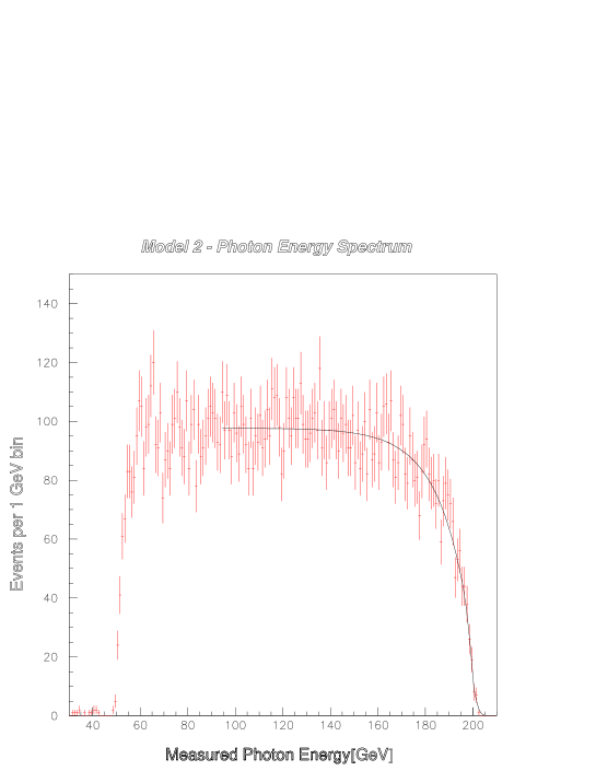
In general, while the most energetic photons will always come from those neutralinos that are directly pair-produced, the lower end of the spectrum will be degraded by the presence of softer photons coming from other SUSY processes, in addition to the SM background (cfr. Sec. 7.8). For this reason, we concentrate here on the upper end of the spectrum to extract the mass. The spectrum which would be obtained after detector effects for 200 GeV neutralino pair production at GeV is shown in Fig. 20 for 200 fb-1 integrated luminosity (corresponding to a run of less than 1 “year” of s). Here we have simulated the SUSY signal that one would detect if Model # 2 was realized. In this case, we have seen in Sec. 2 that fb and all the other SUSY-production processes would be below threshold at GeV.
In order to extract the functional form of the high edge of the spectrum
after ISR, beamstrahlung and detector effects, a much larger number of Monte
Carlo events was used to obtain a fit function using the known mass
as an input. The functional form includes two exponentials
to allow for ISR and beamstrahlung together with a cumulative
normal distribution, Freq, to account for the
calorimeter resolution integrated over the sharp edge of the spectrum.
The function thus obtained was
| (12) | |||||
where and are now free parameters. This functional form was then used to fit to the 200 fb-1 worth of simulated data as shown in Fig. 20 to give the result GeV. To extract the neutralino mass from this measurement we use Eq. (11) to obtain ) GeV. In principle, the mass can also be obtained to high precision at a LC by scanning over the threshold region and previous studies [30] suggest that a precision of order 100 MeV could be obtained from such scans (cfr. also Sec. 5). However, our point here is that even from an early run with a few months worth of data collected at a nominal, fixed c.o.m. energy, a neutralino mass measurement with precision at the level of 2% would be possible.
7.3 Measuring the Neutralino NLSP Decay Length Using 2D Projective Tracking
In this section, we concentrate on determining the average decay length from the distribution of reconstructed two-track events. To this purpose, we require events with at least one photon in the ECAL (coming from one of the two neutralinos produced) and in addition two charged tracks which can be reconstructed to form a vertex (coming from the other neutralino decaying through “charged channels” or to a photon that converts).
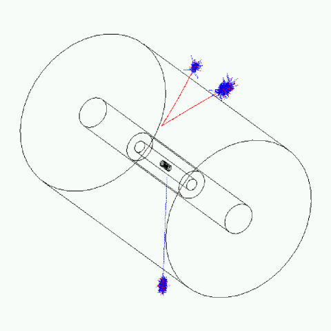
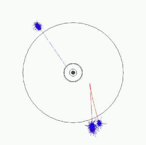
In Fig. 21, we show a representative two-track event among those we generated and fully simulated in the proposed LC detector (3D-view on the left, end-view on the right). This particular event features one displaced photon and a pair coming from a “charged decay”. The non-zero impact parameters of all particles are clearly visible; ECAL showers and tracks are shown (the invisible path is also indicated). Only the vertex detectors and central trackers are displayed.
The detector track hits are provided by the BRAHMS output and these were then formed into tracks and vertices using a home-made reconstruction algorithm. The photon conversion algorithms and multiple scattering effects are internal to BRAHMS and so we have thus implicitly taken full account of the detector material present. However, no special provision was made for multiple scattering or for pattern recognition effects at the reconstruction stage.
We concentrate first on the case of very short lifetimes, less than a few mm, where all the decays take place within the beampipe. In this case, any reconstructed pairs will be due to “charged decays” only and so there will be no confusion arising from conversions. For this region, we must be aware of the beamspot size, which has an rms spread in typically of 400 m, meaning that a three-dimensional decay vertex is no longer useful for lifetime measurements. Instead we must project the decay vertex onto the plane and determine the decay length from the resulting distributions of .
In the following we adopt a conservative approach of using the full GEANT Monte Carlo to generate event samples for a range of true (input to SUSYGEN) decay lengths and then fit the resulting projected lifetime distributions to a simple exponential, plus a constant to allow for long tails. The use of this simple fitting function is conservative in that, once a specific GMSB model is chosen, the projected decay distribution could be chosen exactly and hence fit the data more accurately. Only decay length measurements greater than 10 m are used in the fits, so as to eliminate any residual SM backgrounds with tracks originating from the i.p.
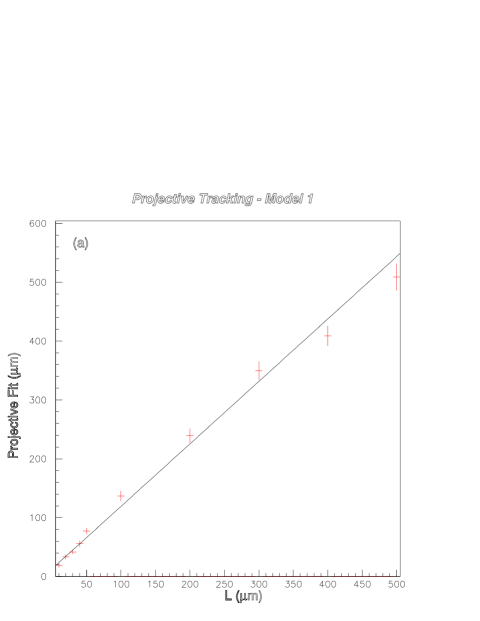
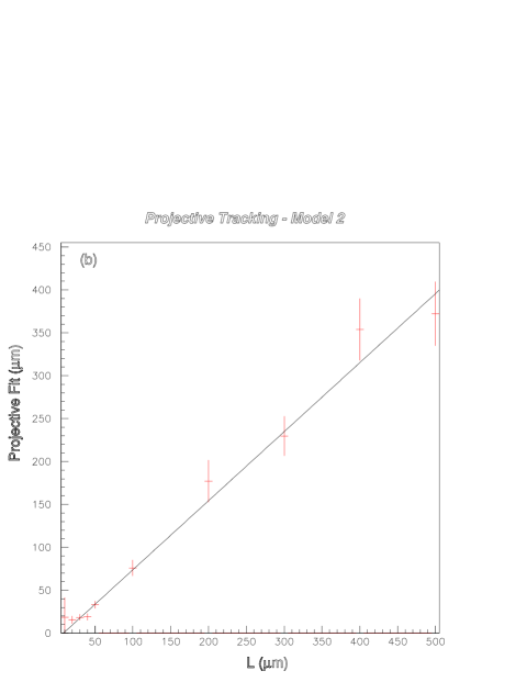
For Model # 1, a set of points were generated using 37,600 (corresponding to 200 fb-1, with fb at GeV) fully simulated events for each point. Note that only the “charged decays” are observed here, because any conversions will take place outside the beampipe, and so the distributions obtained from this sample can be applied directly to any model which has a very short-lived NLSP.
The results are shown in Fig. 22(a) where the outcome of the fits to the projected lifetime is plotted against the true value of . The vertical error bars shown are the parabolic errors obtained from the fit and so correspond to what could be extracted from a run of 200 fb-1. The lifetime is read-off from the fit straight line in order to give the true decay length directly; note that any effects due to ISR or vertexing systematics are included automatically by such a procedure because all these effects are present in the Monte Carlo. This of course also applies to the relativistic factor (). Reading from the plot, the error bars at the 50 m point correspond to a 10% error in the decay length measurement whereas the error bars at 500 m correspond to a 4% error. It can be seen from the straight-line fit to the points that decay lengths down to 30 m are also well-measured for Model # 1.
Performing the same fits to the projected distributions according to Model # 2 with 8,460 events (corresponding to 200 fb-1, with fb at GeV), gives an error of 13% for a 50 m decay length and 10% for a 500 m decay length. The results are shown in Fig. 22(b). It should be noted that, although Model # 2 provides less statistics due to a lower neutralino production cross-section, the possibility of decay to an on-shell boson with subsequent decay to lepton pairs with significant opening angle somewhat compensates for the loss in statistics.
Fig. 22 also shows that lifetimes shorter than 30 m could also be measured in principle using this technique. However it should be remembered that, while the intrinsic beamspot size may be of order 5 nm in and 500 nm in , the actual position of the interation point may have to be determined on a pulse-by-pulse basis which could lead to additional transverse uncertainties. It should also be remembered that we are fitting to track pairs with essentially zero opening angle, which means that simple assumptions about vertex resolution must be avoided. So in the following we remain conservative in our claim that lifetimes as short as 30 m could be measured.
Notice that for Model # 1, the minimum value of allowed by theory is about 110 TeV (cfr. Sec. 3), corresponding to a lifetime of about 200 m and to a decay length m when running at GeV, while for Model # 2, TeV m m. So, our result is that at least for these two particular cases, this method more than covers the lower end of the range for the lifetime. On the other hand, we know that neutralino NLSP models exist where is as short as 5 to 10 m (cfr. Fig. 15 in Sec. 3). For these cases, an alternative approach would be to increase the c.o.m. energy of the machine, hence increasing the boost of the neutralinos, which so far have been close to threshold. In this way, shorter decay lengths factors are readily accessible and would realistically be the preferred approach to measure lifetimes down to 10 m (notice that can never exceed 2.3 for GeV). On the other hand, we checked that GMSB models with a very short lifetime tend to feature a greater degree of degeneracy among the lightest states, so that running at higher energies would also often imply opening other SUSY production channels (-slepton pair production). As a consequence, it is important to address the problem of being able to extract a precise lifetime measurement in the presence of a complex SUSY signal, using appropriate selections.
As an example, we study Model # 3 at GeV with 50,400 total generated events before cuts, corresponding to 200 fb-1, since fb, fb, fb and fb. The events were then selected at the generator level by the following cuts. The events had to contain either exactly two photons with or exactly one photon with and one charged pair of tracks each with . In addition to these cuts, an event which contained any additional particle with was rejected. Afer these cuts the sample contained 21,108 events together with a SUSY “background” of 1,066 selectron pairs, 463 smuon pairs and 336 stau pairs. These events were then passed to the BRAHMS detector simulation followed by the 2D projective fit procedure.
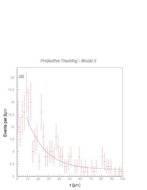
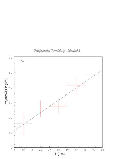
Fig. 23(a) shows the distribution of reconstructed vertex projected radii. The remaining SUSY background consists of only 3 stau events, so its effects are negligible in this case. The error bars for m correspond to 9.8 m. We conclude that for a 200 fb-1 run at GeV, an upper limit on of approximately 20 m could be set at the level. The measurement could of course be improved with higher luminosity together with running at higher energy to utilize a larger () factor. If we could run with fb-1 at 800 GeV, then we could expect a gain of from the statistics together with a gain of 2.2 from an improved (). These would allow a measurement to a precision of approximately 20%.
7.4 Measuring the Neutralino NLSP Decay Length Using 3D Vertexing
For decay lengths greater than about 500 m, the three-dimensional vertex information is useful because the beamspot size in is relatively less important. For this region, photons converting in detector material must be taken into account because these events will appear very similar to the “charged decays”. The vertex position of reconstructed tracks from these two processes are shown in Fig. 24 for Model # 1 with cm.
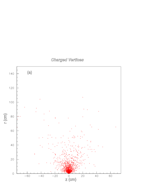
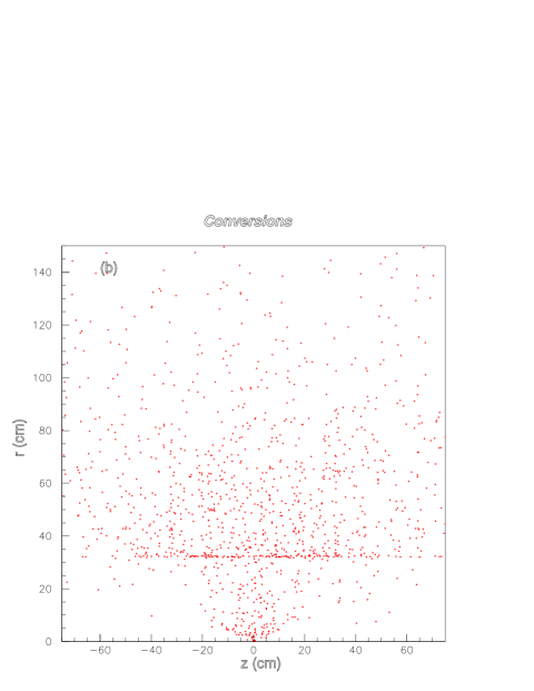
For both the “charged decays” and the conversions, a line of flight can be defined by the lepton-pair vertex and the direction of the reconstructed pair momentum. In the case of conversions, this line of flight reconstructs that of the photon from the neutralino decay. The “charged decays” are also included in this approach effectively as photons which have converted instantly. Referring to Fig. 19(b), is now determined by the energy of the reconstructed pair and we have
| (13) |
In this way a measurement can be obtained for conversions as well as for “charged decays”. However, because we do not wish to make assumptions on the two-track resolution of the central tracker (and hence the reconstruction efficiency for conversions in the outer detector), we prefer here to use only “charged decays” for lifetime determination. However, as shown in Fig. 25(a), we can use the variable as a discriminant. In the following we require to improve the “charged decay” purity.
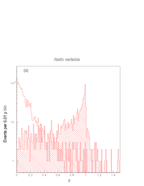
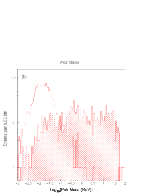
The lepton-pair invariant mass distributions for “charged decays” and conversions are shown in Fig. 25(b) for Model # 1 with cm. Both peak at very low values, of order 10 MeV, for the detector resolutions employed here. However, the conversions are more sharply peaked than the “charged decays”, so cutting on 20 MeV GeV improves the purity of the “charged decay” sample. In addition this cut is desirable because it selects events with a larger opening angle between the daughter tracks, which results in an intrinsically more accurate vertex position measurement. The higher mass cut is to eliminate any residual SM background from leptonic -pair events.
In addition to these cuts we make an additional simple geometrical cut of cm to remove the large number of conversions in the inner TPC wall. After performing these three cuts, the distribution is primarily from the “charged decays” and this is illustrated in Fig. 26, where the fit to Model # 1 with cm is shown. It is clear from this figure that conversions have been reduced to a negligible level.
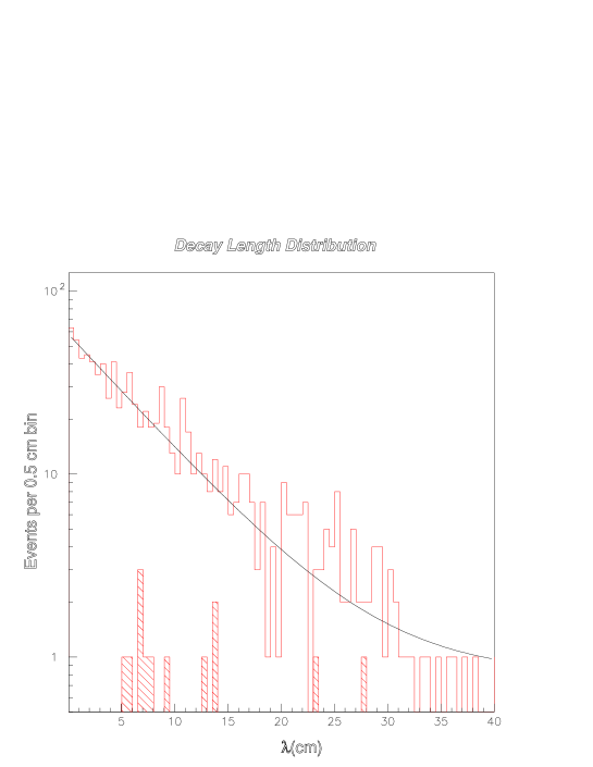
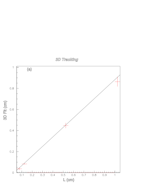
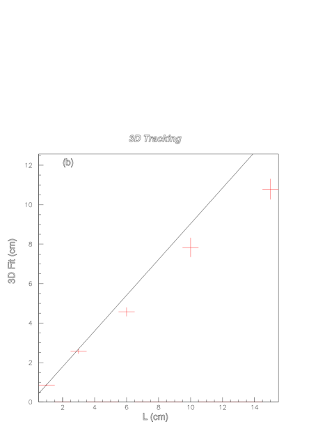
This procedure was repeated for a range of values from 500 m up to 15 cm. The results are shown in Fig. 27 where each point represents the result of the exponential fit, with corresponding errors for samples consisting of 37,600 generated events (200 fb-1) before cuts. The Monte Carlo includes the effects of ISR.
Also shown in Fig. 27 is a straight line fit to the data in (a) which is extrapolated to (b). Using this fit we obtain a relative measurement statistical error of 5% for mm and a relative error of 4% for cm. Our cuts are not optimised for greater than about 10 cm. In this region geometrical detector effects and variations in track reconstruction efficiency become important, as evidenced by the deviation from a straight line in (b). Rather than correct for these effects in detail here, we note that this region of is very well covered by the calorimeter pointing method discussed below.
We conclude that it is possible to make a good measurement (to 10% or better) of nominal decay lengths ranging from 30 m up to 10 cm under very conservative assumptions, using the tracking detectors.
7.5 Measuring the NLSP Decay Length Using Calorimeter
Pointing
A finely segmented ECAL allows for the possibility of detecting photon impact parameters with respect to the i.p. The direction of the photon is reconstructed by fitting to the distribution of energy deposits among the individual ECAL cells which make up the electromagnetic shower. The direction finding is improved significantly by the use of presamplers to provide a precise point along the photon direction. A typical presampler detector consists of lead/scintillating fiber structures which both initiate the shower and measure the point at which the shower begins to a precision of a few tens of m. The use of more than one presampler can provide two points along the photon direction and further improve the direction finding.
In the following, we assume that the angular resolution of the ECAL is that given in Tab. 7. We also need to take account of the spatial and energy resolutions as listed there. Referring to Fig. 19(a), the angle and the distance are determined directly from the calorimeter shower reconstruction. The angle is calculated from the energy of the shower, together with the measured value of the neutralino mass, as described above.
The effect of the mass measurement error was estimated as follows. Each Monte Carlo event was reconstructed using the nominal 100 GeV mass and also using assumed measured masses of 100.1 GeV and 99.9 GeV. We showed in Sec. 7.2 that a mass measurement error of 0.3 GeV could be obtained in a first run of the detector using the upper end of the photon energy spectrum. It would be natural to assume, given any such discovery of neutralino production, that sufficient luminosity would be made available to perform detailed threshold scans and reduce the mass uncertainty to the level of 0.1 GeV (cfr. Sec. 5).
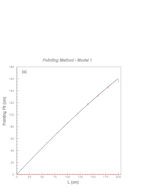
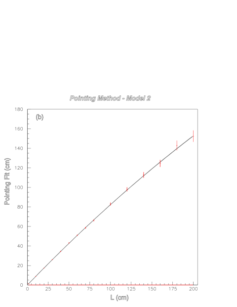
The results are shown in Fig. 28. The Monte Carlo includes effects of ISR and each point was obtained using 37,600 generated events before cuts for Model # 1 and 8,460 events for Model # 2, corresponding to 200 fb-1 for each model running at and 500 GeV, respectively. At each point, the reconstructed decay lengths were fit to an exponential for cm and the points show the fit decay length with corresponding error. The cm cut, corresponding to about for the resolution of this method, serves to reduce any SM background to a negligible level.
The resulting calibration curve is well approximated by a quadratic polynomial and the corresponding fit curves obtained assuming an error on the neutralino mass of MeV are shown together with the points obtained using the correct input masses of 100 GeV for Model # 1 and 200 GeV for Model # 2. In this way the systematic error due to the mass uncertainty is shown to be very small for less than 200 cm for both models. If we examine the lower statistics Model # 2 in the region of cm, we find a statistical error of 6% and in the region of 10 cm we find a statistical error of 1%. Our conclusion is that the calorimeter pointing method works very well for 5 cm m.
7.6 Measuring the NLSP Decay Length Using Calorimeter
Timing
Calorimeter timing information is highly desirable in any detector at a LC in order to reject cosmic rays and many beam-related backgrounds as well as for its use in a trigger. In this section, we investigate a further use of sub-nanosecond timing for neutralino decay length measurement.
For the purposes of this study, we use the energy-dependent timing resolution given in Tab. 7. Referring to Fig. 19, a calorimeter timing measurement gives the quantity . This timing information is then combined with the position and energy measurements, all smeared according to the resolutions given in Tab. 7.
The timing resolution that we use is motivated by what could realistically be achieved for a large calorimeter. This is of the order of 0.5 ns, which naively implies an intrinsic photon impact parameter resolution of order 15 cm. Data sets for a series of decay lengths were simulated using the full Monte Carlo and the reconstructed decay length distributions were fit to a simple exponential between the lengths of 30 cm and 120 cm. The lower limit is given by the timing resolution and the upper limit by the geometrical acceptance of the detector. The results of the fits are shown in Fig. 29. The data points correspond to 200 fb-1 (37,600 and 8,460 generated neutralino pairs at the usual c.o.m. energies for Models # 1 and # 2 respectively, before any cuts are applied). The decay lengths are determined on an event by event basis assuming the exact neutralino mass. The effect of a MeV shift in the input is indicated by the curves, which were obtained by fitting the resulting data points (not shown) to a quadratic polynomial. The results confirm that the effect of neutralino mass uncertainty on a lifetime measurement is small. Values of below 10 cm are poorly determined due to the intrinsic timing resolution and large values of are limited by statistics; the worst case is for Model # 2, where statistics get poor for cm, so we take this as the upper limit for this method.
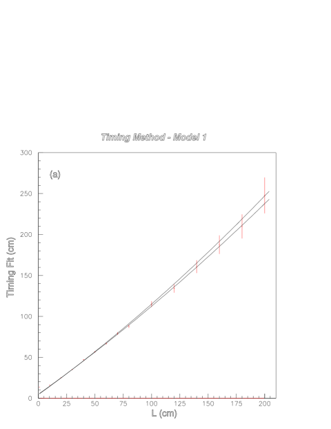
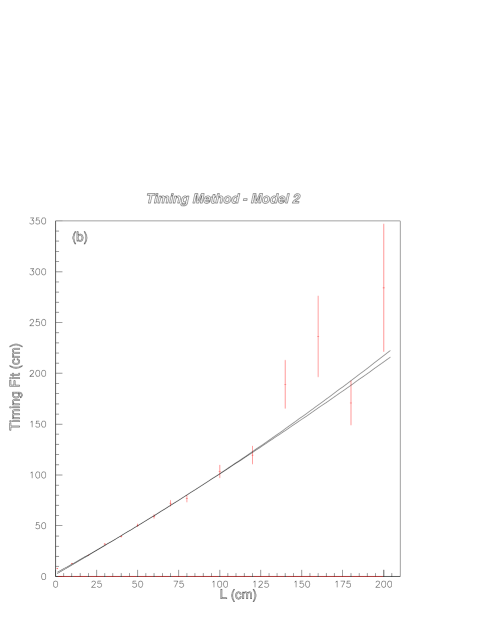
This study shows that timing information alone can not improve on what could be achieved using calorimeter pointing and tracking methods. The timing information could of course be combined with the tracking and pointing methods to achieve an improved accuracy, but we do not consider this further here. We stress, however, that timing should not be neglected in the overall detector design because it may be needed to reduce cosmic ray backgrounds and beam related backgrounds as well as being of use in the trigger for GMSB events. We will further comment on this in the next sections. It is possible that the NLSP is so long-lived that the photon decay would appear in the ECAL several bunch crossings later than expected and indeed not in time with any bunch crossing. To detect such events good timing information would clearly be required.
7.7 Measuring the NLSP Decay Length Using Statistics
A measurement of the NLSP lifetime can also be made using a simple counting technique, because the probability that, e.g., a photon from the decay is observed in the ECAL is a function of the lifetime. As a consequence, the ratio of two-photon to one-photon events observed after SUSY production is a function of the .
As anticipated in Sec. 3 for the spherical detector case, this function is in principle a simple combination of exponentials convoluted with the effects of detector geometry, cuts designed to eliminate SM backgrounds and calorimeter performance. We determine the functional dependence of the ratio using Monte Carlo techniques. Neutralinos were generated from pair production using our modified version of SUSYGEN interfaced to a modified version of CIRCE [38] to include full effects of ISR and beamstrahlung. Any photons coming from decays with energy loosely included in the range given by Eq. (11) and which originated within the detector tracking volume were extrapolated and required to hit within the acceptance of the ECAL. Any event with more than two photons or less than one photon was rejected at this stage. We also imposed cuts on the missing energy, where appropriate, based on the expectations for the signal.
The position of the photons and their energies and angles of pointing were smeared according to the parameters in Tab. 7. The resulting photon impact parameters at the i.p. were then calculated and at least one photon in the event was required to have an impact parameter greater than 30 cm. If one could believe in gaussian statistics to this level, this would correspond to a cut and is hence designed to reduce any SM background to a negligible level (we will further comment on this later in this section).
We define a one-neutralino event as containing one large impact parameter photon and nothing else, and the total number of these events is . We define a two-neutralino event as one where there is at least one large impact parameter photon together with anything else visible in the detector, and the number of these events is . Note that does not include two-photon events only, but also events where both neutralinos decay visibly inside the detector; one of them through and the other through any channel. Our choice is designed to maximise statistics, but we note that simple experimental cuts based on the event topology could easily remove any event which is not purely photonic, should that yield a cleaner analysis. We checked that this would not result in an important loss of statistics (up to about 15% on in the worst cases with a heavy ), so that the essential conclusions of our analysis would remain unchanged. As for , instead, we only include photonic decays because we rely on the presence of a non-pointing photon to eliminate the irreducible radiative SM background, as discussed below.
The ratio was then determined as a function of the neutralino decay length for Models # 1 and # 2 by generating a nominal events running at and 500 GeV, respectively, to start with. The resulting functions are shown in Fig. 30(a).


In order to extract the precision on the measured decay length, we take the error on the measured ratio for the events to be:
| (14) |
and then we obtain
| (15) |
where is the total number of expected events. Note that is not equal to the sum of and because some events will not be counted, due to both neutralinos decaying outside the detector acceptance and/or to non-selected final states.
The resulting curves giving the decay length reach are shown in Fig. 30(b). Assuming an integrated luminosity of 200 fb-1, the plots show that laboratory decay lengths are well measured by this technique down to approximately 50 cm for both models and that the upper limit ranges from approximately 20 m for Model # 2 up to 40 m for Model # 1, corresponding to values of 27 m and 44 m, respectively. It should be noted that the sensitivity of the statistical technique is dependent on the c.o.m energy. The statistics are determined by the quantity , whereas the parameter of physical interest is . We have seen that if we take Model # 2 with c.o.m. energy 500 GeV and allow a maximum measurement error then, as indicated above, we find that we can measure up to 20 m, corresponding to m. If we now decrease the c.o.m energy, then we lose in cross section, but gain in intrinsic sensitivity. In this way, an optimal c.o.m energy can be found for each value of and this optimal energy is plotted against for Model # 2 in Fig. 31(a). The corresponding optimised precision is shown in Fig. 31(b). Unfortunately, it turns out that, at least for Model # 2, any overall gain after optimisation is small. The larger value of that can be measured with a precision of 10% or better is again about 27 m, and the corresponding “optimised” c.o.m. energy is about 463 GeV. While this shows that optimisation gains tend to be small, it also tells us that the method is not critically sensitive to the c.o.m. energy, even though we are running in a threshold region.


To evaluate the level of background reduction we need for a meaningful analysis, let us consider Model # 2 with m and optimise the c.o.m. energy to 463 GeV. At this energy, the corresponding laboratory decay length is m and the production cross section is 25.5 fb. Using 200 fb-1, we obtain the expected values of and . The irreducible backgrounds would need to be subracted from the raw counts involving numbers of this order of magnitude, so we need to check that after a suitable set of cuts the number of background events left is small compared to the statistical errors of about for one neutralino events and for two neutralino events. Experience at LEP (see for example [39]), has shown that backgrounds from cosmic rays and detector noise (sparks and radioactive decays) can be reduced to negligible levels compared to the physics backgrounds by requiring the event timing to be consistent with a beam-crossing. Leaving aside the minor case of events counted in not including 2 photons (they are easily treatable anyway), the SM physics backgrounds are expected to be dominated mainly by events and, to a lesser extent, by radiative bhabha’s. It thus remains to check that the cuts applied in the counting procedure reduce the expected number of events to a “few” events. For this purpose, we performed a quick evaluation of the cross sections for these processes using CompHEP666At this stage, we did not take into account ISR, beamstrahlung effects or any other effects coming from undetected radiation and requiring the following for each photon: a) ; b) included in the range (11). We then found that:
On top of this, one has to take the 30 cm cut on the non-pointing photon impact parameter into account. Of course, it is not reasonable to trust the tails of gaussian statistics so much as to consider this as a real cut. Nevertheless, we note that if we were to “conservatively” evaluate its reduction effect and assume it to be equivalent to an effective cut, the one photon background in 200 fb-1 would still amount to 10 (7) events only for Model # 1 (2), while the two photon background would basically disappear. Hence, we are confident that our set of cuts is strict enough to reduce any background to the level needed for our study to be valid.
While we are aware that detailed studies on non-gaussian tails for calorimeter angular pointing would be highly desirable in order to solve more precisely the background subtraction problem in such a statistical study, we also note that further background reduction is possible before appealing to photon non-pointingness. First, with reference to the most dangerous background, we checked that, after our upper cut on the photon energy in Eq. (11), the remaining contribution from is small and more than 70% of the cross section at GeV comes from pure -exchange (even more than that at GeV). On the other hand, -exchange graphs tend to produce relatively soft photons predominantly along the beam direction, while the signal gives a flat spectrum between the end points (11) and does not show an important angular structure, due to the isotropy of the decay. Based on this, we found that, e.g. for the case of interest for Model # 1 with GeV, imposing stricter cuts GeV and would result in a factor 2 to 3 gain on the signal to background ratio, while the corresponding loss of statistics would be limited to less than 30%.
Second, and most important, there is here a good chance of exploiting the beam polarisation option at the LC. If, on top of the kinematical cuts mentioned above, one could benefit from, say, an 80% polarisation for the electron and a 60% one for the positron, one would get an additional 0.3 or so reduction factor on the dominant -exchange contributions to the one photon background, while the signal would get an enhancement factor, since an important part of it comes from -selectron exchange in the -channel (we remind that our neutralinos are mostly bino’s). If even stronger beam polarisation was available, then one would probably be able to reduce the one photon SM background to an acceptable level by using optimised kinematical cuts and a looser cut on the photon impact parameter such that gaussian statistics could still be trusted.
On the other hand, we checked that the results we obtained for the upper end of our statistical method reach on is not very sensitive to the cut we impose on the photon impact parameter in the 10’s of cm range. The lower end of the reach does, but we know from the previous section that the cm–1 m range is well covered by the direct calorimeter pointing technique. All these considerations make us confident that our statistical study is meaningful and our claim that a measure of with a precision at the level of 10% is possible for typical GMSB models up to several tens of metres by using such a method is safe and possibly even slightly conservative.
Finally, we would like to comment on the fact that larger values of might be accessible by considering a statistical analysis based on the ratio of one (non-pointing) photon events to events where both neutralinos decay outside the detector. Of course, in order to count the latter events, it is necessary that other SUSY processes are within kinematical reach in addition to production, so that events including the visible products of the decays to the NLSP are present. Taking Model # 1 as an example, one could think of running the LC at GeV or so, allowing -slepton pair production followed by (, , ) decays with 100% BR. The resulting SUSY signal would then be made up mainly of , , , and events, where one or both of the non-pointing photons in parentheses coming from may or may not originate within the detector, depending on and the boost for the specific process. For very large neutralino lifetimes, events including two photons are very rare and can be neglected. Note that running at higher c.o.m. energies would increase the factor for ’s coming directly from pair production, resulting in a reduction of from this source, whereas the other processes would produce softer neutralinos with a relatively larger probability of decaying within the detector and contributing to . In addition, the latter processes would provide all the visible SUSY events to be counted as . Hence, the dependence of on would now be affected by the sparticle spectrum and model details, which renders this option less general and more involved than the statistical method based on . In addition, while the SM background to events counted in can still be reduced by requiring large impact parameters for the single photon, such a drastic procedure is not available to reduce the SM contribution to . In the absence of a detailed mSUGRA-like analysis, this would lead to a reduction in the sensitivity to . By quick inspection of Fig. 16 for Model # 1 at GeV, one can get a feeling of the dependence on . Although one should take into account the precise definition of and the differences arising from going to e.g. GeV from 270 GeV, one can still estimate that neutralino lifetimes of the order of 1 km or possibly more might be measurable with some precision by using the statistical method. To further increase statistics and the reach in , one could even consider going to the highest available c.o.m. energies and include all possible processes and cascade decays in the counts. However, this would involve very complex analyses which might be desirable only at a later stage, once it was clear that either the value of to be measured is much larger than the bound suggested by the simple cosmology condition keV or that only an upper limit on can be set. A statistical analysis along these lines, as well as other studies concerning measurements of GMSB parameters at the LHC will also appear soon [40].
7.8 Backgrounds
In this section, we address again the issue of background subtraction and summarize our strategy in this respect for the various techniques described above.
Starting with the very short lifetime and 2D-tracking method case, we note that there are no backgrounds from conversions, because we include only those vertices that occur well within the beampipe with cm ( being the radial coordinate of the vertex) in the exponential fit. Also, any tracks originating from the i.p. should not contaminate the signal, since we impose a cut m when fitting. We also require the invariant mass of the pair of tracks be either less than 10 GeV or in the () GeV range (to retain the peak in the case of Model # 2) to remove any chance of trace backgrounds from leptonic -pair decays with a vertex reconstructed at a distance greater than 10 m from the i.p., due to resolution effects. We also require both leptons to be of the same flavour, which further reduces this background. As for the background, we note that in this case the large invariant mass requires a significant opening angle between the tracks, which makes our 10 m cut on very severe. Any remaining background must then originate from particles with lifetime, such as ’s. However, ’s can only mimic our signal if they decay into 3- (or 5-) prong channels (with 15% BR), which are also mistakenly reconstructed as 2-track events. The effect should be small, but any final detector design should be checked to have sufficient 2-track resolution to ensure that it is negligible. We did not address this and the above problems in detail, because in our study we can safely require the additional presence of a hard [ (45) GeV for Model # 1 (2)] photon coming from the decay of the other neutralino and more than 40 (90) GeV of missing energy, together with selecting only those events where there is nothing else apart from the photon and the reconstructed track pair.
As for the short decay length and 3D-tracking method, the only additional feature compared with the previous case, is the presence of conversions that may or may not be used for the lifetime measurement. We conservatively decided to remove them and we describe our procedure for this in detail in Sec. 7.4. Note also that our cuts here are on the full 3D decay length rather than on the projection .
For intermediate decay lengths (calorimeter pointing/timing methods), the main background arises from the process. All the photons arising from this channel will point to the i.p. and so can be reduced by cutting on the reconstructed decay length . In Sec. 7.5, we achieved this by starting our exponential fits at cm, which corresponds to roughly a 2 cut for the pointing accuracy assumed in our study. In Sec. 7.7, we found that at GeV (for Model # 1) is roughly 31 fb after appropriate cuts, which means that about 1.5 fb are left after the cut. This implies that the remaining background is less than 1% of the signal and so we are safe in our claim that a measurement to 10% or better in the lifetime measurement is possible using these methods. It should be noted that we have assumed gaussian angular resolution for photon pointing and any effects due non-gaussian tails have been neglected. Such residual effects in angular pointing should be included in any future detailed calorimeter studies for the LC detector.
For large decay lengths using the statistical method, we have to address the problem of both and the more severe backgrounds. Any backgrounds due to SM processes will be independent of the neutralino decay length and so the SM contribution can be estimated from Monte Carlo and be subtracted from the measured values of (and ) in our curves in Fig. 30, provided the subtractions are relatively small. To this purpose, in addition to cuts on the photon and missing energies designed to fit the spectrum of the signal, we require a very strict 30 cm cut on the non-pointing impact parameter to reduce the background to a negligible level. This is again somewhat dependent on neglecting non-gaussian tails in the calorimeter resolution. However, in Sec. 7.7, we also discussed in detail possible alternative strategies involving kinematical cut optimisation and beam polarisation.
There remains the question of backgrounds from cosmic rays and beam-related background. As we have mentioned in Sec. 7.7, experience from LEP has shown that cosmics can be rejected provided one can apply good timing information and require no hadronic energy in the event. In addition, the background from cosmics (and beam-related backgrounds or calorimeter noise) can be estimated using random dedicated triggers and subtracted if necessary. Additional veto walls could be constructed around the detector to kill any remaining muonic background, if the above measures proved insufficient.
7.9 Summary
We have shown in this section that a general purpose detector operating at a LC with c.o.m. energies in the 200–500 GeV range could provide a good lifetime measurement, to 10% or better, over 6 orders of magnitude, from tens of m to tens of m for a few representative scenarios. We have based this on a 200 fb-1 run, corresponding, e.g., to approximately 1 year at the high luminosity proposed for TESLA and a few years at JLC/NLC.

The techniques we have used in the study are summarised in Fig. 32, as a function of the average decay length. It can be seen that while a wide range (e.g. 30 m–40 m for Model # 1) can well be covered by using individual techniques, there is also significant overlap for many of the intermediate regions. This implies important redundancy in the lifetime measurement and the opportunity to combine results to achieve an even greater precision.
For many cases (e.g. Model # 1), this is more than enough to cover the lower end of the theoretically allowed range for and the upper end as well, if naive cosmological constraints are imposed. On the other hand, we recognise that scenarios with very short lifetimes at the level of a few m are possible in the context of GMSB and in this case one can either set an upper limit or push for higher LC energies to maximise the relativistic factor (facing however more complex analyses in the presence of competing SUSY signals).
We have also considered scenarios where the gravitino mass is heavier than keV and consequently the neutralino has a very long lifetime ’s of metres. For these cases, we have proposed a way to slightly extend the reach by running the LC at a c.o.m. energy optimised with respect to the relativistic boost factor and a simple statistical analysis, but we have seen that a solid improvement can only come from increasing the available integrated luminosity. Interesting prospects for a measurement of very large values of up to km also exist, based on a more complex statistical analysis in a SUGRA-like scenario where most produced NLSP’s appear stable and are invisible, but there is still a non-negligible number of neutralinos undergoing a decay within the detector.
Referring to Eq. (8), we note that a 10% error in corresponds to a 3% error in . This is of the same order of magnitude as the theoretical uncertainty on the factor introduced in Sec. 3. In comparison, the contributing error from the neutralino mass measurement using the threshold-scanning technique or the method of Sec. 7.2 is negligible.
Hence we conclude that, for the models considered and under conservative assumptions, it is possible to determine with a precision of approximately 5% by only performing lifetime and mass measurements in the context of GMSB with neutralino NLSP. Less model dependent results can be obtained by adding information on the physical composition from other observables, such as decay BR’s, cross sections etc.
8 Conclusions
After introducing the GMSB framework and discussing the region of the parameter space of interest for LC searches, we focused on the case of a neutralino NLSP and demonstrated how measurements made at the LC can provide information on the detailed structure of the theory at both the electroweak and the very high energy scales.
We have shown how a study of the SUSY particle mass spectrum, measured e.g. via threshold-scanning techniques, can allow the determination of the fundamental GMSB parameters with high precision. In an explicit example where many SUSY thresholds can be explored running at GeV, we found that accuracies at the level of 0.1% for and , 1% for and 1–2% for are achievable.
In particular, we stressed the possibility of performing a measurement of the lifetime at the LC with the aim of extracting information also on the SUSY breaking sector of the theory and its fundamental scale . To this purpose, we studied main and rare decay channels in detail and set up specific simulation tools based on the TESLA/CDR proposals. Using representative GMSB models, we then found that can be measured to 10% or better over a large range, from tens of m to tens of m, which in many cases covers the scenarios allowed from the theory and suggested by simple cosmological arguments. (We also sketched a possible way to treat the case where 10’s m km.) We showed that this, together with a mass measurement to (whose feasibility at the LC we also demonstrated), yields a 5% determination of under conservative assumptions, if minimal GMSB-model constraints are used. Better and less model dependent results can also come from analyses of other observables such as decay BR’s, cross sections etc.
Our results in this respect and the reach in depend on details of the detector design, which we assumed to be general-purpose oriented. For instance, for intermediate lifetimes, we obtained a very high accuracy using calorimeter pointing/timing techniques. It should be noted, however, that our calorimeter pointing precision has assumed the presence of pre-shower detectors, while simple calorimetry alone might not be sufficient for our purpose.
On the other hand, extreme cases allowed by the GMSB framework with very short (few m) or very long ( km) lifetime require special detector design. For the very short case, one should consider the feasibility of upgrading the interaction region to include smaller beampipe radii combined with ultimate vertexing technology. Better performances for the very long case can only be achieved by having electromagnetic calorimetry at larger distances from the i.p.. This points to either a larger detector or dedicated additional devices, e.g. lead scintillator arrays or similar, possibly well separated from the main detector (a proposal in this direction for the D0 experiment at the Tevatron has already been discussed in Ref. [41]). If clear SUSY signals are detected at the LHC and/or during the first phase of LC operations, then it should be possible to distinguish scenarios with a stable (e.g. mSUGRA) from GMSB scenarios with a very long-lived NLSP and large by measuring and studying the sparticle spectrum or other observables. If the indications favour a GMSB pattern, then the addition of dedicated devices at large distances would be highly desirable for later LC runs. In this case, the position of the detector in the experimental hall as well as the dimensions of the hall itself should be cleverly designed to allow for such improvements.
Our study clearly shows that high luminosity at the LC, such as that proposed for TESLA is very desirable in order to allow both a better accuracy in extracting the GMSB parameters from detailed knowledge of the sparticle spectrum and a good precision measurement of the NLSP lifetime in (most of) the range suggested by theory. Indeed, we checked that any reduction in luminosity would significantly eat away at both ends of the reach, while the situation would improve perceivably if even higher luminosities could be available.
We have pointed out that the clean environment and the flexibility of an collider are ideal to achieve precise measurements in this respect in a variety of GMSB scenarios. In particular, we made strong use of the LC ability of running at a variable c.o.m. energy to benefit from SUSY thresholds for both measuring the GMSB spectrum and for facilitating the lifetime measurement. Also, for the latter measurement, the precise knowledge of the production energy was essential and we note that this technique is not available at a hadron collider.
Finally, we would like to stress that the present study turned out to be an ideal benchmark for developing software intended for the TESLA/CDR detector simulation that is expected to be broadly used for future analyses of general interest. We have indeed seen that all parts of the detector are potentially involved in the measurement of the NLSP lifetime and unusual and extreme performance and precision have been often required, as e.g. in the analysis based on tracking for the very short case. Again, we note that the usefulness of the software and algorithms we developed for our purposes in GMSB is in many cases extendable to other new physics scenarios, such as general LESB models or -parity violation. Also, our analysis could hopefully trigger new, non-standard ideas during the detector design process, in order to improve the performance for the measurements we described without reducing the effectiveness of the apparatus for other tasks.
Acknowledgements
We acknowledge useful conversations with Alan Caldwell, Thomas Gehrmann, Sven Heinemeyer, Graham Kribs, Steve Martin, Frank Paige, Tilman Plehn, Michael Plümacher, Sasha Pukhov, Nicholas Walker, Katherine Wipf. We would like to thank especially Peter Zerwas for many suggestions as well as for constant encouragement and support.
References
- [1] For a recent pedagogical review of supersymmetry and supersymmetry breaking, see S. P. Martin, “A Supersymmetry Primer”, in “Perspectives on Supersymmetry”, G. L. Kane ed., World Scientific 1998, hep-ph/9709356 and references therein.
- [2] See, e.g., G. L. Kane, C. Kolda, L. Roszkowski, J. D. Wells, Phys. Rev. D 49 (1994) 6173.
- [3] For a recent review, see G. F. Giudice, R. Rattazzi, “Theories with Gauge-Mediated Supersymmetry Breaking”, hep-ph/9801271, submitted to Phys. Rep.
- [4] P. Fayet, Phys. Lett. 70B (1977) 461; Phys. Lett. 86B (1979) 272; Phys. Lett. B 175 (1986) 471 and in “Unification of the fundamental particle interactions”, eds. S. Ferrara, J. Ellis, P. van Nieuwenhuizen (Plenum, New York, 1980) p. 587.
- [5] See, e.g., J. Ellis, K Enqvist, D. Nanopoulos, Phys. Lett. B 147 (1984) 99; A. B. Lahanas, D. V. Nanopoulos, Phys. Rep. 145 (1987) 1; J. L. Lopez, D. V. Nanopoulos, A. Zichichi, Phys. Rev. Lett. 77 (1996) 5168; hep-ph/9610235; Phys. Rev. D 55 (1997) 5813; J. L. Lopez, D. V. Nanopoulos, hep-ph/9701264; J. Kim et al., Phys. Rev. D 57 (1998) 373.
- [6] M. Dine, W. Fischler, M. Srednicki, Nucl. Phys. B189 (1981) 575; S. Dimopoulos, S. Raby, Nucl. Phys. B192 (1981) 353; M. Dine, W. Fischler, Phys. Lett. 110B (1982) 227; M. Dine, M. Srednicki, Nucl. Phys. B202 (1982) 238; M. Dine, W. Fischler, Nucl. Phys. B204 (1982) 346; L. Alvarez-Gaumé, M. Claudson, M. B. Wise, Nucl. Phys. B207 (1982) 96; C. R. Nappi, B. A. Ovrut, Phys. Lett. 113B (1982) 175; S. Dimopoulos, S. Raby, Nucl. Phys. B219 (1983) 479.
- [7] M. Dine, A. E. Nelson, Phys. Rev. D 48 (1993) 1277; M. Dine, A. E. Nelson, Y. Shirman, Phys. Rev. D 51 (1995) 1362; M. Dine, A. E. Nelson, Y. Nir, Y. Shirman, Phys. Rev. D 53 (1996) 2658.
- [8] S. Dimopoulos, S. Thomas, J. D. Wells, Phys. Rev. D 54 (1996) 3283; Nucl. Phys. B488 (1997) 39.
- [9] J. A. Bagger, K. Matchev, D. M. Pierce, R. Zhang, Phys. Rev. D 55 (1997) 3188.
- [10] S. Ambrosanio, G. L. Kane, G. D. Kribs, S. P. Martin and S. Mrenna, Phys. Rev. D 54 (1996) 5395.
- [11] S. Ambrosanio, G. D. Kribs, S. P. Martin, Phys. Rev. D 56 (1997) 1761.
- [12] S. Park, “Search for New Phenomena in CDF”, 10th Topical Workshop on Proton-Antiproton Collider Physics, R. Raja and J. Yoh (eds.), AIP Press, New York (1995); CDF Collaboration, Phys. Rev. Lett. 81 (1998) 1791; hep-ex/9806034.
- [13] S. Dimopoulos, M. Dine, S. Raby and S. Thomas, Phys. Rev. Lett. 76 (1996) 3494; S. Ambrosanio, G. L. Kane, G. D. Kribs, S. P. Martin and S. Mrenna, Phys. Rev. Lett. 76 (1996) 3498.
- [14] For an overview of recent searches at LEP, see e.g.: Joint LEP SUSY Working Group webpage http://www.cern.ch/lepsusy/.
- [15] For an overview of recent D0 searhces at the Tevatron, see e.g.: http://www-d0.fnal.gov/public/new/analyses/gauge.
- [16] See, e.g., the LESB-GMSB Working Group webpage for the recent “Physics at Run II: SUSY/Higgs” Workshop: http://fnth37.fnal.gov/gm/gmrun2.html.
- [17] See e.g.: H.Baer, P. G. Mercadante, F. Paige, X. Tata, Y. Wang, Phys. Lett. B 435 (1998) 109; I. Hinchliffe, F. E. Paige, hep-ph/9812233.
- [18] See e.g.: H. Pagels, J. R. Primack, Phys. Rev. Lett. 48 (1982) 223.
- [19] For inquiries about this software package, please send e-mail to ambros@mail.cern.ch.
- [20] A relevant example is discussed in: S. Ambrosanio, G. D. Kribs and S. P. Martin, Nucl. Phys. B516 (1998) 55.
- [21] H. E. Haber and G. L. Kane, Phys. Rep. 117 (1985) 75, and Erratum, SCIPP 85/47.
- [22] See, e.g.: G. Dvali, G. F. Giudice, A. Pomarol, Nucl. Phys. B478 (1996) 31.
- [23] S. P. Martin, Phys. Rev. D 55 (1997) 3177.
- [24] E. Accomando et al. [The ECFA/DESY LC Physics Working Group], Phys. Rep. 299 (1998) 1.
-
[25]
LanHEP was downloaded from the webpage
http://theory.npi.msu.su/ semenov/lanhep.html. See also A. V. Semenov, “LanHEP: A Package for Automatic Generation of Feynman Rules”, hep-ph/9608488, and updates MSU-98-2/503. - [26] E. E. Boos, M. N. Dubinin, V. A. Ilin, A. E. Pukhov, V. I. Savrin, “CompHEP: Specialized package for automatic calculation of elementary particle decays and collisions”, hep-ph/9503280, and references therein; P. A. Baikov et al., “Physical results by means of CompHEP”, Proc. of X Workshop on High Energy Physics and Quantum Field Theory (QFTHEP-95), B. Levtchenko, V. Savrin eds. (Moscow, 1996), p. 101 (hep-ph/9701412). Version 3.3.18 is preliminary and was downloaded from the webpage http://theory.npi.msu.su/ comphep (courtesy of A. E. Pukhov).
- [27] The MSSM lagrangian created by means of LanHEP (version last corrected on Nov. 14, 1998) was downloaded from the webpage http://theory.npi.msu.su/ semenov/mssm.html. An older version of the lagrangian was presented in A. S. Belyaev et al., hep-ph/9712303.
- [28] S. P. Martin, private communication, unpublished.
- [29] See, e.g., the webpage: http://lcwws.physics.yale.edu/lc.
- [30] “Conceptual Design of a 500 GeV Linear Collider with Integrated X-ray Laser Facility”, R. Brinkmann, G. Martelik, J. Rossbach, A. Wagner eds., DESY 1997-048, ECFA 1997-182.
-
[31]
See the webpage
http://www.desy.de/ njwalker/ecfa-desy-wg4/parameter_list.html - [32] See e.g. Ref. [30], vol. 1, pag. 219–222.
- [33] See e.g. H. E. Haber, R. Hempfling, A. H. Hoang, Z. Phys. C 75 (539) 1997; S. Heinemeyer, W. Hollik, G. Weiglein, hep-ph/9812472.
-
[34]
Consult the webpage
http://wwwinfo.cern.ch/asd/cernlib/minuit. -
[35]
SUSYGEN 2.20/03 was downloaded from the webpage
http://lyohp5.in2p3.fr/delphi/katsan/susygen.html. -
[36]
For inquiries about this software package, please send e-mail to
g.blair@rhbnc.ac.uk or consult the webpage
http://www.hep.ph.rhbnc.ac.uk/ blair/detsim/brahms.html. - [37] Consult the webpage http://wwwinfo.cern.ch/asdoc/geantold/GEANTMAIN.html.
- [38] “CIRCE Version 1/02: Beam Spectra for Simulating Linear Collider Physics”, hep-ph/9607454.
- [39] The ALEPH collaboration, Phys. Lett. B 313 (1993) 520.
- [40] F. Paige, private communication. These studies will be included in the supersymmetry section of the chapter about the ATLAS detector and physics performance in vol. II of the “ATLAS Technical Design Report”, 1999.
- [41] C. H. Chen, J. F. Gunion, Phys. Lett. B 420 (1998) 77; Phys. Rev. D 58 (1998) 075005.