May 17, 1999

Study of leptoquark pair production at the LHC with the CMS detector

Salavat Abdullin ^a), François Charles ^b)

Groupe de Recherche en Physique des Hautes Energies

Université de Haute Alsace, 61 rue A.Camus 68093 Mulhouse, France

We study the discovery potential of the CMS detector for the scalar leptoquark pair production at the LHC. Present and future exclusion limits are considered. We find that the maximal leptoquark mass reach is m $\simeq$ 1.47 TeV for the branching ratio of Br(LQ_l $\rightarrow$ l q) = 100 %, while for Br(LQ_l $\rightarrow$ l q) = 50 % the upper limit is 1.2 TeV for an integrated luminosity of 100 fb^-1. We obtain comparable results for electron and muon-type leptoquarks. The pileup effect at high luminosity is discussed.

^a) Email: adullin@mail.cern.ch
^b) Email: charles@in2p3.fr

1 Introduction and phenomenology

Leptoquark particles appear in extensions of the Standard Model like Grand Unified Theories, composite models and R-parity violating Supersymmetry. They carry both lepton and baryon number. These particles mediate transition between quark and lepton . Leptoquarks can be scalar (Spin= 0) or vector (Spin=1) and couple to leptons via a Yukawa type coupling. These particles conserve lepton and baryon number in order to avoid a fast proton decay. One can classify the different leptoquark through their spin, weak isospin and fermion number, see details in [1, 2].

In the following we consider only pair production of scalar leptoquarks: almost no dependence on the $\lambda$ coupling is expected (coupling to lepton and quark). The leptoquark resonance width can be defined as ([1]):

$\Gamma\simeq 350MeV\frac{\lambda^{2}}{4\pi\alpha}\frac{M_{LQ}}{200GeV}$

We obtain $\Gamma\simeq$ 2 GeV for $\lambda$ = $\sqrt{4\pi\alpha}$ and M_LQ = 1200 GeV. As we will see later the theoretical width is overwhelmed by the calorimeter resolution. If we assume that leptoquarks have either left or right couplings but not both, the branching fraction is 0, 0.5 or 1 for symmetry reason. We consider both electron and muon leptoquark type with Br(LQ_e $\rightarrow$ e q) = 1 or Br(LQ_e $\rightarrow$ e q) = 0.5 and Br(LQ_μ $\rightarrow$ $\mu$ q) = 1 or Br(LQ_μ $\rightarrow$ $\mu$ q) = 0.5.

Fig.1 shows the leading-order diagrams for the leptoquark pair production at LHC. One can notice that except for the diagram of the type $q\bar{q}\rightarrow LQ\bar{LQ}$ via e-exchange, all the other processes do not depend on the $\lambda$ coupling (only vertex $g-LQ-\bar{LQ}$). This is very important as the cross section then depend mainly on the mass of the leptoquark.

Figure 1: Leptoquark pair production diagrams

We take the total cross section for the leptoquark pair production from [3] (Next-to-Leading Order calculations (NLO) using CTEQ4M structure function). The difference between LO (as in PYTHIA [4]) and NLO can reach $50\%$ depending on the leptoquark mass. Thus NLO cross section is taken for our analysis.

2 Exclusion limit

The current limit on the leptoquark originates from HERA and Tevatron [5, 6] analysis. At the Tevatron the exclusion limit for NLO cross section is investigated by both CDF and DO [7]. Combining both results one obtains : M${}_{LQ}^{Scalar}>$ 246 GeV. We can expect at $\sqrt{s}$ = 2 TeV with L = 1 fb^-1 for the Tevatron (D0+CDF) a limit of M${}_{LQ}^{Scalar}>$ 350 GeV.

At LEP the exclusion limit was investigated, e.g., by OPAL using the fact that the leptoquark enhances the cross section of e⁺e^- $\rightarrow q\bar{q}$ in t/u channel exchange [8]. A preliminary study carried out in CMS [9] showed that the mass reach is about 1.5 TeV [10]. Several studies have been done to evaluate the LHC performance of leptoquark detection: [11, 12, 13]. The study presented in this note includes a more accurate detector performance description (as will be explained in next section), takes into account all sources of background and includes superposition of events at high luminosity (so called pileup).

3 Simulation and CMSJET/CMSIM comparison

Fig.2 shows the full GEANT simulation of a 900 GeV leptoquark pair decay into electron (positron) and u ($\bar{u}$) quark jet ($pp\rightarrow LQ_{e}\bar{LQ_{e}}\rightarrow e^{-}e^{+}u\bar{u}$) in the CMS detector.

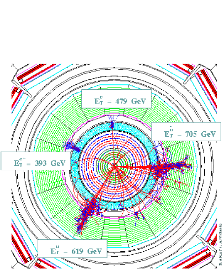
Figure 2: Full GEANT simulation of $pp\rightarrow LQ_{e}\bar{LQ_{e}}\rightarrow e^{-}e^{+}u\bar{u}$ for m${}_{LQ_{e}}$ = 900 GeV.

The CMSJET fast Monte-Carlo package [14] is used to model the CMS detector response due to the huge sample of events to be processed (about 20 millions at generator level and half a million at the simulation level). The fast simulation incorporates the full granularity of the calorimeter with an energy smearing according to GEANT simulation and parameterization of the longitudinal and lateral profiles of showers with some cracks description (transition regions of calorimeter: endcap-barrel, endcap-forward calorimeter), charged particles and the muon resolution is parameterized as function of $p_{T}$ and $\eta$. Here we illustrate the performance of the fast simulation with some distributions in Fig.3, where the 1 TeV jet response is produced by both fast simulation with CMSJET and full detector simulation with CMSIM [15]. We compare the energy resolution, transverse energy distribution (i. e. the ratio of the energy contained in a cone of $R=\sqrt{\eta^{2}+\phi^{2}}$ value to the total energy) and the fraction of the jet energy deposited in electromagnetic calorimeter.

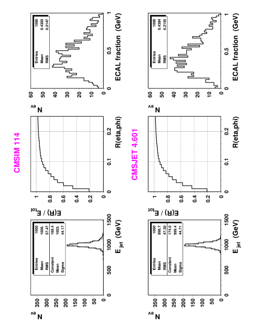
Figure 3: Full simulation versus fast simulation for 1 TeV jets

.

4 Background

The background processes considered in the following are required to have 2 isolated high-p_T leptons and at least 2 energetic jets. Due to the large QCD cross section, semileptonic decays of heavy flavour are also considered requiring isolated high-p_T leptons (coming from jets).

In Tab.1 we give the cross section for some processes where the production of 2 leptons and 2 jets is forced in PYTHIA. For some processes with a very large total cross section the generated samples are subdivided in several $\hat{p}_{T}$ intervals.

Due to the large QCD cross section a special treatment is applied for those events. After parton generation and hadronization each meson with sufficient value of p_T is decayed 1000 times in order to select events where at least 2 high-p_T leptons (p${}_{T}>$ 40 GeV) of same flavour and opposite sign (SF OS) are produced (see Tab.2). Once passes this requirement the QCD event is processed through CMSJET simulation. This procedure increases the generated statistics by a factor 1000. After this simulation no QCD event survives the first level selection: 2 isolated high-p_T leptons (p${}_{T}>$ 40 GeV in $|\eta|<$ 2.4) of opposite sign and same flavour and at least 2 jets ( E${}_{T}>$ 40 GeV in $|\eta|<$ 4.5).

Process	ZZ(ll jj)	ZW(ll jj)	$t\bar{t}$(l $\nu$ j	Zjet	Wbt(l $\nu$ l $\nu$ jj)	WW(l $\nu$ l $\nu$)
			l $\nu$ j)	($\hat{p_{T}}>$ 20 GeV)	($\hat{p_{T}}>$ 20 GeV)
$\sigma$ (fb)	600	596	$7\cdot 10^{3}$	$1.25\cdot 10^{5}$	$10^{3}$	827
Number of events	$6\cdot 10^{4}$	$6\cdot 10^{4}$	$7\cdot 10^{5}$	$1.25\cdot 10^{7}$	$10^{5}$	$8.27\cdot 10^{4}$
Nbr of gen. evts	$1.8\cdot 10^{5}$	$1.8\cdot 10^{5}$	$10^{6}$	$8.4\cdot 10^{6}$	$2\cdot 10^{5}$	$10^{5}$

Table 1: Background cross section and number of events for L = 10⁵ pb^-1.

Kinematics	$\sigma$ (fb)	gen evts	ratio
$100$ $GeV<\hat{p_{T}}<200$ $GeV$	$1.3\cdot 10^{9}$	$1.1\cdot 10^{9}$	$0.01$
$200$ $GeV<\hat{p_{T}}<400$ $GeV$	$7.14\cdot 10^{7}$	$1.6\cdot 10^{8}$	$0.02$
$\hat{p_{T}}>400$ $GeV$	$2.8\cdot 10^{6}$	$1.24\cdot 10^{8}$	$0.44$

Table 2: QCD cross section and number of events for $L=100$ $fb^{-1}$

5 Selection variables

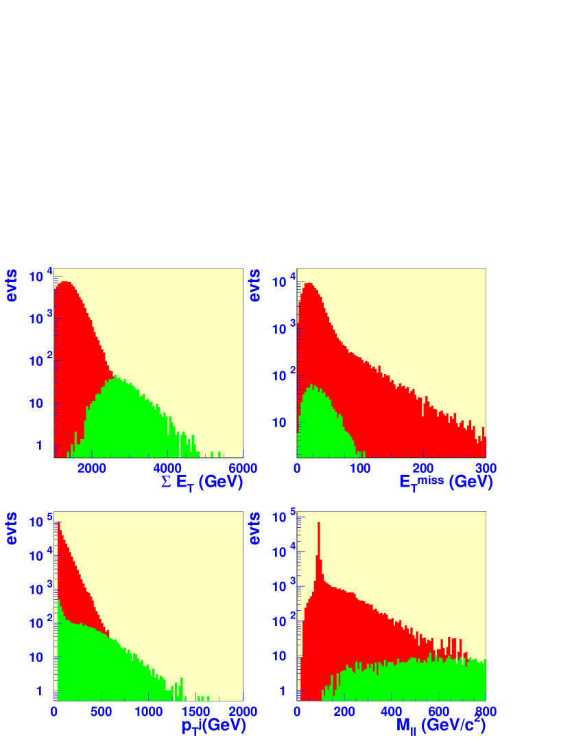
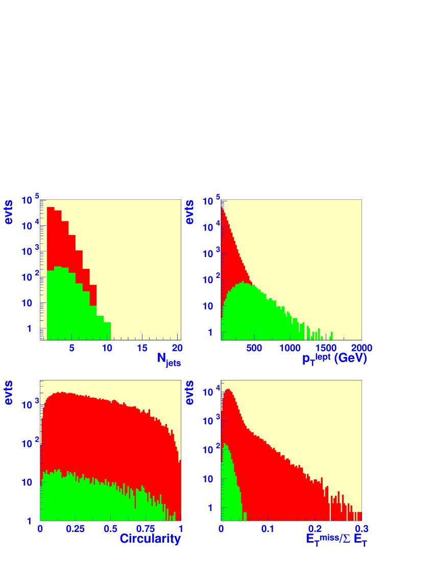
Figure 4: Distributions over selection variables (signal in light grey and background in dark grey, m${}_{LQ_{e}}$ = 900 GeV).

The selection is based on several basic variables with different cut values to optimize the signal over background ratio for various leptoquark masses. We require exactly 2 isolated leptons SF OS with p${}_{T}>$ 40 GeV and at least 2 jets with E${}_{T}>$ 40 GeV (so called first level cuts). Fig.4 shows some distributions after applying first level cuts for signal (leptoquark pair production of m${}_{LQ_{e}}$ = 900 GeV) and background. In order to reduce the background originating from Z decay in 2 leptons we apply the lepton pair mass cut: m${}_{ll}>$ 100–200 GeV. The $t\bar{t}$ background is reduced by constraining the missing transverse energy to a low value : E${}_{T}^{miss}<$ 80–150 GeV. This reduces the amount of events where an energetic neutrino is produced. We also use the variable $\Sigma$ E_T which is the sum of the event ( cell by cell) transverse energy in the calorimeter system down to $|\eta|$ = 4.5. The requirement on this value takes into account the pileup (see next section for details) which produces a shift of about 800 GeV, so we impose: $\Sigma$ E${}_{T}>$ 1500–2000 GeV. We also use the ratio of the last two variables to cope with the fact that the transverse missing energy tail in the case of balanced events ( no energetic neutrino ) originates mainly from a mismeasurement of high energy jets. Thus the variable E${}_{T}^{miss}/\Sigma$ E_T should be suitable to solve this problem as illustrated in Fig.4 . We require : E${}_{T}^{miss}/\Sigma$ E${}_{T}<$ 0.03–0.05.

One of the most important requirement is related to the characteristics of pair production, therefore both pairs of the lepton-jet invariant mass has to be within a window: $\Delta$ m${}_{lj}<$ 150–320 GeV. Finally, in order to obtain the best significance we search for a signal peak as an excess of events over exponentially falling background distribution with an optimised window: $\Delta$m $<$ 100–220 GeV. The procedure to obtain the best significance for several leptoquark mass values makes use of a loop over the previous cuts. Here we consider all the possible combinations between the 2 leptons and the jets (at least 2), resulting sometimes in more than 2 accepted lepton-jet pairs in one event. The same treatment is applied to the signal and to the background.

A typical selection for m_LQ = 1400 GeV is based on the following cuts:

• 2 isolated leptons (SF OS) with p${}_{T}>$ 40 GeV, $|\eta|<$ 2.4; m${}_{ll}>$ 150 GeV

• At least 2 jets with E${}_{T}>$ 60 GeV , $|\eta|<$ 4.5

• E${}_{T}^{miss}<$ 185 GeV, $\Sigma$ E${}_{T}>$ 1700 GeV, E${}_{T}^{miss}$/$\Sigma$ E${}_{T}<$ 0.04

• $\Delta$ m${}_{lj}<$ 310 GeV, the peak window $\Delta$m = 210 GeV

6 Effect of pileup on the observables

The pileup originates from the fact that several protons can interact during the same bunch crossing. Assuming a total proton-proton cross section of 100 mb at the LHC (from a Regge-based extrapolation of low energy data) and taking into account the time interval between bunch crossing of 25 ns, we obtain an average of 25 interactions per bunch crossings (Poisson distribution) for an instantaneous luminosity of 10³⁴ cm^-2s^-1. In our simulation we superimpose these events produced with MSEL=2 by PYTHIA (it includes elastic scattering, single and double diffraction).

The effect on the signal can be seen in Fig.5, where the dashed line corresponds to the case when the pileup is not included and the continuous line to the one with pileup included. The upper two plots show the efficiency of the lepton isolation in the pileup conditions, i.e the fraction of isolated leptons with pileup relative to one without pileup as function of the rapidity and transverse momentum of leptons. In the lower two plots the effect of pileup on the missing transverse energy and total transverse energy is illustrated. Pileup has a small effect on E${}^{miss}_{T}$ distribution as minimum bias events are well balanced. On the other hand, it increases the $\Sigma$ E_T value by an average value of $\sim$ 800 GeV.

The most noticeable effect of pileup is the degradation of the lepton isolation. The isolation definition includes a rejection at the tracking and at the calorimeter level. For the tracking we require no charged particle with a $p_{T}>$ 2 GeV in a cone $\Delta$R $<$ 0.3 around the electron track (assuming 100 % track-finding efficiency). At the calorimeter level we require less than 10 % of the electron energy in cone 0.05 $<\Delta$R $<$ 0.3 around the electron barycenter. On average the isolation efficiency is about 85 % . It is relatively independant on the rapidity but increases with p_T to reach a plateau.

Figure 5: Pileup effect on isolation efficiency of electrons, on E${}_{T}^{miss}$ and $\Sigma$ E_T (solid line corresponds to no-pileup case, dashed line - to the pileup included).

7 Results for electron and muon type leptoquark

The following results are obtained for muon and electron scalar leptoquarks, Tab.3.  A global $95\%$ efficiency for the lepton reconstruction ( $\epsilon_{rec}^{e}=0.95$ ) is assumed, based on the results of a detailed GEANT study. We deduce a limit of 1470 GeV for a branching ratio of 1 and a limit of 1200 GeV for a branching ratio of 0.5, taking more stringent criterion of the 5 $\sigma$ excess in terms of $\frac{S}{\sqrt{S+B}}$. For muon type we obtain the same results within less than 10 GeV. In Fig.6 one can see the lepton-jet invariant mass distributions for the Standard Model (SM) background combined with the leptoquark signal for various leptoquark masses : 600 GeV, 900 GeV, 1.2 TeV and 1.5 TeV after applying the first level cuts and requiring m${}_{ll}>$ 150 GeV. The contributions (%) of the various SM background processes after all cuts as function of the leptoquark mass are given in Tab.4, where (a) corresponds to the $\hat{p_{T}}>$100 GeV, (b): 50 GeV $<\hat{p_{T}}<$100 GeV and (c): 20 GeV $<\hat{p_{T}}<$ 50 GeV.

MLQ (GeV)	900	1200	1400	1500
Signal	2584	174.4	49	24.6
Background	240	45.27	11.3	7.5
$\sigma=\frac{S}{\sqrt{S+B}}$	49	11.8	6.3	4.34
$\sigma=\frac{S}{\sqrt{B}}$	167	25.9	14.6	9.0

Table 3: Number of accepted $lj$ combinations and significance for L = 100 fb^-1 for electron type leptoquark.

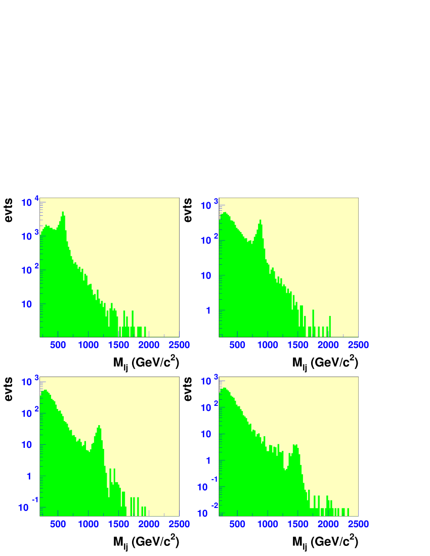
Figure 6: Invariant lepton-jet mass distributions after first level cuts and m${}_{ll}>$ 150 GeV for several signal leptoquark masses (600, 900, 1200 and 1500 GeV) with expected SM background included.

Proc.	$t\bar{t}$	Zjet (a)	Zjet (b)	Zjet (c)	ZZ	WW	Wbt
M${}_{LQ_{e}}(GeV)$
600	28	60.6	8.7	1.2	0.4	0.3	0.8
900	16.4	74.6	7.6	0	0.2	0	1.1
1200	10.1	89.9	0	0	0	0	0
1300	4.2	95.8	0	0	0	0	0
1400	0	100	0	0	0	0	0
1500	0	100	0	0	0	0	0

Table 4: Background composition in percents for electron type leptoquark after all cuts

8 Mass peak and calibration

In order to obtain the width we fit the mass distribution for signal only with a gaussian, as the energy resolution dominates over the intrinsic Breit Wigner. The leptoquark mass can be approximately described as:

$M_{LQ}=\sqrt{(\tilde{p_{l}}+\tilde{p_{jet}})^{2}}\simeq\sqrt{2E_{l}E_{j}(1-cos\theta)}$

From this relation we can deduce that $\frac{\sigma(M_{LQ})}{M_{LQ}}\simeq\frac{\sigma(E_{j})}{2E_{j}}$ due to the excellent lepton energy resolution in CMS. Therefore the width of the leptoquark peak is approximately a half of the jet energy resolution. For high masses, high energy jets and excluding the Hadron Forward calorimeter(HF) region ($|\eta|>3$), we expect the constant term to dominate the jet energy resolution. This means that we have (outside of cracks and barrel-endcap region):

$\frac{\sigma(M_{LQ})}{M_{LQ}}\simeq\frac{6.5\%}{2}=3.25\%$.

This is in good agreement with the Fig.7, where, for example, we obtain $\sigma$ = 42 GeV for M_LQ = 1.3 TeV.

We plot in Fig.7 the lepton-jet invariant mass applying first level cuts and m${}_{ll}>$ 400 GeV, E${}_{T}^{miss}<$ 180 GeV, $\Sigma$ E${}_{T}>$ 1500 GeV, E${}_{T}^{miss}/\Sigma$E${}_{T}<$ 0.04. The underestimation of the leptoquark mass is mainly due to the finite cone jetfinder and to be corrected by calibration procedure.

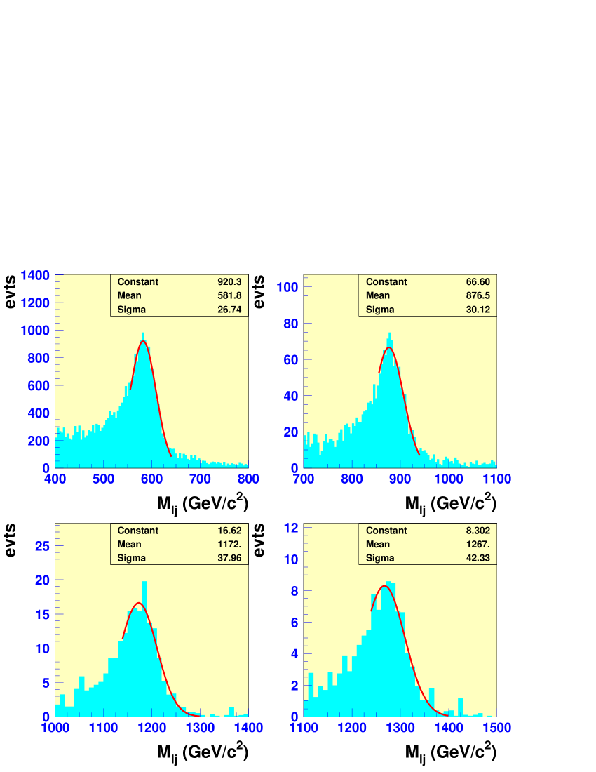
Figure 7: Leptoquark mass resolution for generated masses of 600, 900, 1200 and 1300 GeV.

9 Conclusion

The scalar leptoquark is expected to be observed in CMS detector up to M_LQ $\simeq$ 1.5 TeV for 100 fb^-1 and assuming Br(LQ $\rightarrow$ e q) = 100 %. The study of the electron and muon leptoquark type gives similar results. The width of the leptoquark mass peak depends on the leptoquark mass and is expected to be about $\sigma$ = 42 GeV at M_LQ =1.3 TeV. Pileup effect has limited influence, reducing mainly the lepton isolation efficiency and shifting $\Sigma$E_T value.

More details of this study can be found in CMS NOTE available on CMS information server [16]

References

- [1] R. Ruckl and H. Spiesberger, CERN-TH/97-322, hep-ph/9711352.
- [2] W. Buchmuller et al., Phys. Lett. B191 (1987) 442.
- [3] J. Bluemlein, E. Boos and A. Kryukov, DESY 97-067, hep-ph/9811271.
- [4] T. Sjostrand, Computer Phys. Comm. 82 (1994) 74.
- [5] H1 Collaboration, Proc. ICHEP98.
- [6] M. Kramer et al., Phys.Rev.Lett.79 (1997) 341.
- [7] CDF and D0 Collaborations, FERMILAB-PUB-98-312-E.
- [8] OPAL Collaboration, Eur.Phys.J. C2 (1998) 441.
- [9] CMS collaboration, Technical Proposal, CERN/LHCC 94-38.
- [10] G. Wrochna, CMS CR-1996/003.
- [11] O.J.P. Eboli, R.Z. Funchal and T.L Lungov, Phys.Rev. D57 (1998) 1715.
- [12] B. Dion et al., Eur.Phys.J. C2 (1998) 497.
- [13] B. Dion, L. Marleau and G. Simon, Phys.Rev. D59 (1999) 015001.
-
[14]
S. Abdullin, A. Khanov and N. Stepanov, CMS TN-1994/180,
http://cmsdoc.cern.ch/abdullin/cmsjet.html. - [15] http://cmsdoc.cern.ch/cmsim/cmsim.html
-
[16]
S. Abdullin and F. Charles, CMS NOTE-1999/027,
http://cmsdoc.cern.ch/docnotes.shtml.