1 Introduction

It is a prediction of the theory of Quantum Chromodynamics (QCD) that at hadron colliders the production of Drell-Yan pairs or weak gauge bosons ($W^{\pm}$ and $Z$) will generally be accompanied by gluon radiation. Therefore, in order to test QCD theory or the electroweak properties of vector bosons, it is necessary to include the effects of multiple gluon emission. At the Fermilab Tevatron (a $p\bar{p}$ collider), we expect about $2\times 10^{6}$ $W^{\pm}$ and $6\times 10^{5}$ $Z$ bosons produced at $\sqrt{S}=1.8$ TeV, per $100\,{\rm pb}^{-1}$ of luminosity. This large sample of data is useful (i) for QCD studies (with either single or multiple scales), (ii) as a tool for precision measurements of the $W$ boson mass and width, and (iii) as a probe for new physics (e.g., $Z^{\prime}$). Achievement of these physics goals requires accurate predictions for the distributions of the rapidity and the transverse momentum of $W^{\pm}/Z$ bosons and of their decay products.

Consider the production process $h_{1}h_{2}\rightarrow VX$. Denote $Q_{T}$ and $Q$ to be the transverse momentum and the invariant mass of the vector boson $V$, respectively. When $Q_{T}\sim Q$, there is only one hard scale and a fixed-order perturbation calculation is reliable. When $Q_{T}\ll Q$, there are two hard scales and the convergence of the conventional perturbative expansion is impaired. Hence, it is necessary to apply the technique of QCD resummation to combine the singular terms in each order of perturbative calculation, which yields:

$$\frac{d\sigma}{dQ_{T}^{2}}\sim\frac{1}{Q_{T}^{2}}\left\{\right.\alpha_{S}(L+1) +\alpha_{S}^{2}(L^{3}+L^{2}) +\alpha_{S}^{3}(L^{5}+L^{4})+\alpha_{S}^{4}(L^{7}+L^{6})+...$$

$$+\alpha_{S}^{2}(~{}L+~{}~{}1) +\alpha_{S}^{3}(L^{3}+L^{2})+\alpha_{S}^{4}(L^{5}+L^{4})+...$$

$$+\alpha_{S}^{3}(~{}L+~{}~{}1)+\alpha_{S}^{4}(L^{3}+L^{2})+...\left.\right\},$$

where $\alpha_{s}$ is the strong coupling constant, $L$ denotes $\ln(Q^{2}/Q_{T}^{2})$ and the explicit coefficients multiplying the logs are suppressed.

Resummation of large logarithms yields a Sudakov form factor [1, 2] and cures divergences as $Q_{T}\rightarrow 0$. This resummation was pioneered by Dokshitzer, D’yakonov and Troyan (DDT) who performed an analysis in $Q_{T}$-space which led to a leading-log resummation formalism [1]. Later, Parisi-Petronzio showed [2] that for large $Q$ the $Q_{T}\rightarrow 0$ region can be calculated perturbatively by imposing the condition of transverse momentum conservation,

$$\delta^{(2)}\left(\sum_{i=1}^{n}{\vec{k}_{T_{i}}}-{\vec{q}_{T}}\right)=\int{d^{2}b\over 4\pi^{2}}\;\textstyle{e}^{i{\vec{Q}_{T}}\cdot{\vec{b}}}\prod_{i=1}^{n}\;\textstyle{e}^{i{\vec{k}_{T_{i}}}\cdot{\vec{b}}},$$ (2)

in $b$-space ($b$ is the impact parameter, which is the Fourier conjugate of $Q_{T}$). Their improved formalism also sums some subleading-logs. They showed that as $Q\rightarrow\infty$, events at $Q_{T}\sim 0$ may be obtained asymptotically by the emission of at least two gluons whose transverse momenta are not small and add to zero. The intercept at $Q_{T}=0$ is predicted to be [2]

$$\left.\frac{d\sigma}{dQ_{T}^{2}}\right|_{Q_{T}\rightarrow 0}\sim\sigma_{0}\left({\Lambda^{2}\over Q^{2}}\right)^{\eta_{0}},$$ (3)

where $\eta_{0}=A\ln\left[1+{1\over A}\right]$ with $A=12C_{F}/(33-2n_{f})$, and $\eta_{0}\simeq 0.6$ for $n_{f}=4$ and $C_{F}=4/3$. Collins and Soper extended [3] this work in $b$-space and applied the properties of the renormalization group invariance to create a formalism that resums all the large log terms to all orders in $\alpha_{s}$.

Although various formalisms for resumming large $\ln(Q^{2}/Q^{2}_{T})$ terms have been proposed in the literature [4, 5], we will concentrate in this paper on the formalism given by Collins, Soper and Sterman (CSS) [6], which has been applied to studies of the production of single [7, 8, 9, 10] and double [11] weak gauge bosons as well as Higgs bosons [12] at hadron colliders.

2 Collins-Soper-Sterman Resummation Formalism

In the CSS resummation formalism, the cross section is written in the form

$${\frac{d\sigma(h_{1}h_{2}\rightarrow VX)}{dQ^{2}\,dQ_{T}^{2}dy\,\,}}={\frac{1}{(2\pi)^{2}}}\int d^{2}b\,e^{i{\vec{Q}_{T}}\cdot{\vec{b}}}{\widetilde{W}(b,Q,x_{1},x_{2})}+~{}Y(Q_{T},Q,x_{1},x_{2}),$$ (4)

where $y$ is the rapidity of the vector boson $V$, and the parton momentum fractions are defined as $x_{1}=e^{y}Q/\sqrt{S}$ and $x_{2}=e^{-y}Q/\sqrt{S}$ with $\sqrt{S}$ as the center-of-mass (CM) energy of the hadrons $h_{1}$ and $h_{2}$. In Eq. (4), $Y$ is the regular piece which can be obtained by subtracting the singular terms from the exact fixed-order result. The quantity ${\widetilde{W}}$ satisfies a renormalization group equation with the solution of the form

$${\widetilde{W}(Q,b,x_{1},x_{2})}=e^{-{\cal S}(Q,b{,C_{1},C_{2}})}{\widetilde{W}\left(\frac{C_{1}}{C_{2}b},b,x_{1},x_{2}\right)}.$$ (5)

Here the Sudakov exponent is defined as

$${\cal S}(Q,b{,C_{1},C_{2}})=\int_{C_{1}^{2}/b^{2}}^{C_{2}^{2}Q^{2}}\frac{d\overline{\mu}^{2}}{\overline{\mu}^{2}}\left[{A}\left({\alpha}_{s}(\overline{\mu}),C_{1}\right)\ln\left(\frac{C_{2}^{2}Q^{2}}{\overline{\mu}^{2}}\right){+B}\left({\alpha}_{s}(\overline{\mu}),C_{1},C_{2}\right)\right],$$ (6)

and the $x_{1}$ and $x_{2}$ dependence of $\widetilde{W}$ factorizes as

$${\widetilde{W}\left(\frac{C_{1}}{C_{2}b},b,x_{1},x_{2}\right)}=\sum_{j}e_{j}^{2}\;{\cal C}_{jh_{1}}\left(\frac{C_{1}}{C_{2}b},b,x_{1}\right)\;{\cal C}_{jh_{2}}\left(\frac{C_{1}}{C_{2}b},b,x_{2}\right).$$ (7)

Here, ${\cal C}_{jh}$ is a convolution of the parton distribution function ($f_{a/h}$) with calculable Wilson coefficient functions ($C_{ja}$), which are defined through

$${\cal C}_{jh}(Q,b,x)=\sum_{a}\int_{x}^{1}{\frac{d\xi}{\xi}}\;C_{ja}\left(\frac{x}{\xi},b,\mu={C_{3}\over b},Q\right)\;f_{a/h}\left(\xi,\mu={C_{3}\over b}\right).$$ (8)

The sum on the index $a$ is over incoming partons, $j$ denotes the quark flavors with (electroweak) charge $e_{j}$, and the factorization scale $\mu$ is fixed to be $C_{3}/b$. A few comments about this formalism:

• The $A$, $B$ and $C$ functions can be calculated order-by-order in $\alpha_{s}$.

• A special choice can be made for the renormalization constants $C_{i}$ so that the contributions obtained from the expansion in $\alpha_{s}$ of the CSS resummed calculation agree with those from the fixed-order calculation. This is the canonical choice. It has $C_{1}=C_{3}=2e^{-\gamma_{E}}\equiv b_{0}$ and $C_{2}=C_{1}/b_{0}=1$, where $\gamma_{E}$ is Euler’s constant.

• $b$ is integrated from 0 to $\infty$. For $b\gg 1/\Lambda_{QCD}$, the perturbative calculation is no longer reliable. In order to account for non-perturbative contributions from the large $b$ region this formalism includes an additional multiplicative factor which contains measurable parameters.

We refer the readers to Ref. [9] for a more detailed discussion on how to apply the CSS resummation formalism to the phenomenology of hadron collider physics.

2.1 The Non-perturbative Function

As noted in the previous section, it is necessary to include an additional factor, usually referred to as the “non-perturbative function”, in the CSS resummation formalism in order to incorporate some long distance physics not accounted for by the perturbative derivation. Collins and Soper postulated [6]

$$\widetilde{W}_{j{\bar{k}}}(b)=\widetilde{W}_{j{\bar{k}}}(b_{*})\widetilde{W}_{j{\bar{k}}}^{NP}(b)\,,$$ (9)

with

$$b_{*}={\frac{b}{\sqrt{1+(b/b_{max})^{2}}}}\,,$$ (10)

so that $b$ never exceeds $b_{max}$ and $\widetilde{W}_{j{\bar{k}}}(b_{*})$ can be reliably calculated in perturbation theory. (In numerical calculations, $b_{max}$ is typically set to be of the order of $1~{}{\rm GeV}^{-1}$.) Based upon a renormalization group analysis, they found that the non-perturbative function can be generally written as

$$\widetilde{W}_{j\bar{k}}^{NP}(b,Q,Q_{0},x_{1},x_{2})=\exp\left[-F_{1}(b)\ln\left(\frac{Q^{2}}{Q_{0}^{2}}\right)-F_{j/{h_{1}}}(x_{1},b)-F_{{\bar{k}}/{h_{2}}}(x_{2},b)\right]\,,$$ (11)

where $F_{1}$, $F_{j/{h_{1}}}$ and $F_{{\bar{k}}/{h_{2}}}$ must be extracted from data with the constraint that

$$\widetilde{W}_{j\bar{k}}^{NP}(b=0)=1.$$

Furthermore, $F_{1}$ only depends on $Q$, while $F_{j/{h_{1}}}$ and $F_{{\bar{k}}/{h_{2}}}$ in general depend on $x_{1}$ or $x_{2}$, and their values can depend on the flavor of the initial state partons ($j$ and $\bar{k}$ in this case). Later, in Ref. [13], it was shown that the $F_{1}(b)\ln\left(\frac{Q^{2}}{Q_{0}^{2}}\right)$ dependence is also suggested by infrared renormalon contributions to the $Q_{T}$ distribution.

2.2 Testing the Universality of $\widetilde{W}_{j\bar{k}}^{NP}$

The CSS resummation formalism suggests that the non-perturbative function should be universal. Its role is analogous to that of the parton distribution function (PDF) in any fixed order perturbative calculation, as its value must be determined from data. The first attempt to determine such a universal non-perturbative function was made by Davies, Webber and Stirling (DWS) [14] in 1985 who fit data available at that time to the resummed piece (the $\widetilde{W}_{j\bar{k}}$ term) Duke and Owens parton distribution functions [15]. Subsequently, the DWS results were combined with a NLO calculation [16] by Arnold and Kauffman [7] in 1991 to provide the first complete CSS prediction relevant to hadron collider Drell-Yan data. In 1994, Ladinsky and Yuan (LY) [17] observed that the prediction of the DWS set of $\widetilde{W}_{j\bar{k}}^{NP}$ deviates from R209 data ($p+p\rightarrow\mu^{+}\mu^{-}+X$ at $\sqrt{S}=62$ GeV) using the CTEQ2M PDF [18]. In order to incorporate possible $\ln(\tau)$ dependence, LY postulated a model for the non-perturbative term, which was different from that of DWS, as

$$\widetilde{W}_{j\bar{k}}^{NP}(b,Q,Q_{0},x_{1},x_{2})={\rm exp}\left[-g_{1}b^{2}-g_{2}b^{2}\ln\left({\frac{Q}{2Q_{0}}}\right)-g_{1}g_{3}b\ln{(100x_{1}x_{2})}\right],$$ (12)

where $x_{1}x_{2}=\tau$. A “two-stage fit” of the R209, CDF-$Z$ ($4\,{\rm pb}^{-1}$ data) and E288 ($p+Cu$) data gave [17]

$$g_{1}=0.11_{-0.03}^{+0.04}~{}{\rm GeV}^{2}\;,\;g_{2}=0.58_{-0.2}^{+0.1}~{}{\rm GeV}^{2}\;,\;g_{3}=-1.5_{-0.1}^{+0.1}~{}{\rm GeV}^{-1},$$

for $Q_{0}=1.6~{}{\rm GeV}$ and $b_{max}=0.5~{}{\rm GeV}^{-1}$. The purpose of the project described here is to update these non-perturbative parameters using modern, high-statistics samples of Drell-Yan data and to incorporate a fitting technique which will track the full error matrix for all fitted parameters. Our results are given in the following sections.

3 Fitting Procedure

3.1 Choice of the Parametrization Form

At the present time, the non-perturbative functions in the CSS resummation formalism cannot be derived from QCD theory, so a variety of functional forms should be studied. The only necessary condition is that $\widetilde{W}_{j\bar{k}}^{NP}(b=0)=1$. For simplicity, we consider only two typical functional forms for $\widetilde{W}_{j\bar{k}}^{NP}(b,Q,Q_{0},x_{1},x_{2})$ in $b$ space: (i) 2-parameter pure Gaussian form [DWS form]:

$${\rm exp}\left[-g_{1}-g_{2}\ln\left({\frac{Q}{2Q_{0}}}\right)\right]b^{2}\,,$$ (13)

with $Q_{0}=1.6$ GeV; and (ii) a 3-parameter form [LY form]:

$${\rm exp}\left\{\left[-g_{1}-g_{2}\ln\left({\frac{Q}{2Q_{0}}}\right)\right]b^{2}-\left[g_{1}g_{3}\ln\!{(100x_{1}x_{2})}\right]b\right\}\,,$$ (14)

with a logarithamic $x$-dependent third term which is linear in $b$. This is equivalent to $\ln({\tau}/{\tau_{0}})$ for $\tau_{0}=0.1$.

Both forms assume no flavor dependence for simplicity. In addition to fitting for the non-perturbative parameters, $g_{1},\,g_{2},\,\mbox{and}\,g_{3}$, the overall normalizations were allowed to float for some fits. One can also study another pure Gaussian form with similar $x$ dependence such as

$${\rm exp}\left[-g_{1}-g_{2}\ln\left({\frac{Q}{2Q_{0}}}\right)-g_{1}g_{3}\ln{(100x_{1}x_{2})}\right]b^{2}\,.$$

However, we find that current data are not yet precise enough to clearly separate the $g_{2}$ and $g_{3}$ parameters within this functional form and so it is not considered here. We also tested a few additional functions which did not incorporate additional parameters, but did not find any clear advantage to them when fitting the current Drell-Yan data. However, as to be shown later, the Run 1 $W$/$Z$ data at the Tevatron are expected to determine the $g_{2}$ coefficient with good accuracy, and these data can be combined with the low energy Drell-Yan data to further test various scenarios for $x$ dependence and ultimately, universality.

3.2 Choice of the Data Sets

In order to determine the non-perturbative functions discussed above, we need to choose experimental data sets for which the contribution to the non-perturbative piece dominates the transverse momentum distributions. This suggests using low energy fixed target or collider data in which the transverse momentum ($Q_{T}$) of the Drell-Yan pair is much less than its invariant mass ($Q$). Because the CSS resummation formalism better describes data in which the Drell-Yan pairs are produced in the central rapidity region (as defined in the center-of-mass frame of the initial state hadrons) we shall concentrate on data with those properties. Based upon the above criteria we chose to consider data shown in Table 1.

Experiment	reference	Reaction	$\sqrt{S}$ GeV	$\langle\tau\rangle$	$\delta N$
R209	[22]	$p+p\rightarrow\mu^{+}\mu^{-}+X$	62	$\sim 0.1$	10%
E605	[23]	$p+Cu\rightarrow\mu^{+}\mu^{-}+X$	38.8	$\sim 0.2$	15%
CDF-$Z$	[24]	$p+\bar{p}\rightarrow Z+X$	1800	$\sim 0.05$	–
E288	[25]	$p+Cu\rightarrow\mu^{+}\mu^{-}+X$	27.4	$\sim 0.2$	25%

Table 1: Drell-Yan data used in this analysis. Here, $\delta N$ is the published normalization uncertainty for each experiment. The CDF data were from Tevatron collider Run 0 of 4 pb^-1.

We have also examined the E772 data [19], from the process $p+H^{2}\rightarrow\mu^{+}\mu^{-}+X$ at $\sqrt{S}=56.6$ GeV, and found that it was not compatible in our fits with the above data, and it is not included in this study. Except where noted, all of the fits to $g_{1,2,3}$ were done using the CTEQ3M PDF [21] fits.

Figure 1: R209 data, from $p+p\rightarrow\mu^{+}\mu^{-}+X$ at $\sqrt{S}=62$ GeV, with an overall systematic normalization error of $10\%$. The curves are the results of Fit $A_{2}$ and $A_{3}$ and are multiplied by the value of NORM, as shown in the figure and described in the text.

Figure 2: Comparison of $4\,{\rm pb}^{-1}$ CDF-$Z$ data at the Tevatron with two different theory model predictions. The dots correspond to the results of Fit $A_{2}$ and $A_{3}$.

Figure 3: E605 data, from $p+Cu\rightarrow\mu^{+}\mu^{-}+X$ at $\sqrt{S}=38.8$ GeV, with an overall systematic normalization error of $15\%$. The curves are the results of Fit $A_{2}$ and $A_{3}$ and are multiplied by the value of NORM, as shown in the figure and described in the text.

3.3 Primary Fits

As to be shown later, the E288 data have the smallest errors, and would be expected to dominate the result of a global fit. That is indeed the case. When including the E288 data in a global fit, we found that the resulting fit required the NORM to be too large (as compared to the experimental systematic error) for either the E288 or the E605 data. Furthermore, the shape of the R209 data cannot be well described by the theory prediction based on such a fit.

3.3.1 Fits $A_{2,3}$

We therefore employed a different strategy for the global fit based on the statistical quality of the data. We included the first two mass bins ($7<Q<8$ GeV and $8<Q<9$ GeV) of the E605 data and all of the R209 and the CDF-$Z$ boson data, in an initial global fit, referred to here as Fit $A_{2,3}$. In total, 31 data points were considered. We allowed the normalization of the R209 and E605 data to float within their overall systematic normalization errors, while fixing the normalization of the CDF-$Z$ data to unity. (The point-to-point systematic error of 10% for the E605 data has also been included in the error bars of the data points shown in Fig. 3.) In addition to the normalization factor for each experiment, the fitted parameters of our global fit include the coefficients $g_{1,2}$ and $g_{1,2,3}$ for the 2-parameter and 3-parameter fits, respectively. We found that, for $Q_{0}=1.6$ GeV and $b_{max}=1/(2\,{\rm GeV})$, both the 2-parameter and the 3-parameter forms give good fits, with $\chi^{2}$ per degree of freedom about equal to 1.4. The best fitted central values for Fit $A_{2}$ are: $g_{1}=0.24~{}{\rm GeV}^{2}\;,\;g_{2}=034~{}{\rm GeV}^{2}$. While the central values for Fit $A_{3}$ are $g_{1}=0.15~{}{\rm GeV}^{2}\;,\;g_{2}=0.48~{}{\rm GeV}^{2}\;,\;g_{3}=-0.58~{}{\rm GeV}^{-1}$. The fitted values for NORM are 1.04 for both Fits $A_{2}$ and $A_{3}$.

3.3.2 Uncertainties in the Fits

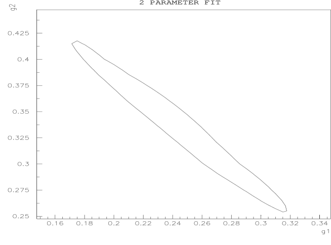
Figure 4: The error ellipse on the $g_{1}$ and $g_{2}$ plane from which the errors of the 2-parameter fit $A_{2}$ were interpreted.

(a)

(b)

(c)

Figure 5: The error ellipse projections from which the errors of the 3-parameter fit $A_{3}$ were interpreted. (a) $g_{1}$ and $g_{2}$ plane, (b) $g_{2}$ and $g_{3}$ plane, and (c) $g_{1}$ and $g_{3}$ plane.

We have also studied the uncertainties of the fitted $g$ parameters. For the 2-parameter fit, the $1\sigma$ error in the $\chi^{2}$ plot (with an approximately elliptical contour) gives $-0.07<\delta g_{1}<0.08~{}{\rm GeV}^{2}$ and $-0.08<\delta g_{2}<0.07~{}{\rm GeV}^{2}$. For the 3-parameter fit, the situation is more complicated, as the fitted values of $g$’s are highly correlated. In order to estimate the uncertainties of the fitted $g$ values, we fix the value (at its best fit value) of $g$’s, one at a time, and examine the uncertainties of the other two, in a way similar to studying the 2-parameter fit result. We found that

$$\mbox{$g_{1}$ fixed:}-0.05 < \delta g_{2}<0.04~{}{\rm GeV}^{2}\;,$$

$$-0.02 < \delta g_{3}<0.26~{}{\rm GeV}^{-1}\;;$$

$$\mbox{$g_{2}$ fixed:}-0.02 < \delta g_{1}<0.03~{}{\rm GeV}^{2}\;,$$

$$-0.08 < \delta g_{3}<0.07~{}{\rm GeV}^{-1}\;;$$

$$\mbox{$g_{3}$ fixed:}-0.02 < \delta g_{1}<0.04~{}{\rm GeV}^{2}\;,$$

$$-0.03 < \delta g_{2}<0.02~{}{\rm GeV}^{2}\;;$$

constitute a conservative set of uncertainty ranges. With the understanding of the complexity discussed above, we characterize the uncertainties of the fitted $g$’s in the 3-parameter form conservatively by their maximal deviations, so that the best fitted $g$ values are:

$${\rm Fit}\;A_{2}:$$

$$g_{1} = 0.24^{+0.08}_{-0.07}~{}{\rm GeV}^{2}\;,\;g_{2}=034^{+0.07}_{-0.08}~{}{\rm GeV}^{2}\;;$$

$${\rm Fit}\;A_{3}:$$

$$g_{1} = 0.15^{+0.04}_{-0.03}~{}{\rm GeV}^{2}\;,\;g_{2}=0.48^{+0.04}_{-0.05}~{}{\rm GeV}^{2}\;,\;g_{3}=-0.58^{+0.26}_{-0.20}~{}{\rm GeV}^{-1}\;;$$

for the 2 and 3 parameter fits, respectively. In Figs. 4 and 5, we show the error ellipse projections from which we interpreted the errors of the above fits. In summary, fits $A_{2}$ and $A_{3}$ constitute the main results of this paper.

3.3.3 Cross Checks

Figure 6: E288 data, from $p+Cu\rightarrow\mu^{+}\mu^{-}+X$ at $\sqrt{S}=27.4$ GeV, with an overall systematic normalization error of $25\%$. The curves are the results of Fit $N_{1}$ and $N_{2}$ and are multiplied by the value of NORM, as shown in the figure and described in the text.

Given these values of $g$’s and the fitted normalization factors for the E605 data, we can calculate the two different predictions for the other three high mass bins not used in Fits $A_{2,3}$, and the results are also shown in Fig. 3. In order to compare with the E288 data, we created Fits $N_{2,3}$ in which we fix the $g$’s to those obtained from Fit $A_{3}$ and fit for NORM from the E288 data alone. Fig. 6 shows the resulting fits are acceptable, with values of NORM close to the quoted 25%, namely, NORM$=0.92$ and $0.79$ for Fits $N_{2,3}$, respectively. It is encouraging that the quality of the fit for the E288 results is very similar to that for the E605 data and that the normalizations are now acceptably within the range quoted by the experiment. Hence, we conclude that the fitted values of $g$’s reasonably describe the wide-ranging, complete set of data, as discussed above.

We note that although the CDF-$Z$ data, as shown in Fig. 2, contain only 7 data points with large statistical uncertainties, they prove to be very useful in determining the value of $g_{2}$. To test this observation, we performed an additional fit, $L_{2}$. Following the method suggested in [17], we set $g_{3}$ to be zero and fit the $g_{1}$ and $g_{2}$ parameters using the R209 and CDF-$Z$ data alone. (Note that for the R209 data, the typical value of $\tau$ is of the order 0.1, which motivates the choice of $\tau_{0}=0.1$ in the LY form. Effectively, the $g_{3}$ contribution to the R209 data can be ignored.) We found that the best fit gives $g_{2}=0.47~{}{\rm GeV}^{2}$, which is in good agreement with the result of the global Fit $A_{3}$ discussed above. Hence, we conclude that the CDF-$Z$ data already play an important role in constraining the $g_{2}$ parameter, which can be further improved with a large $Z$ data samples from Run 1 of the Tevatron collider experiments. We shall defer its discussion to the next section.

4 Run 1 $W$ and $Z$ Boson Data at the Tevatron

The Run 1 $W$ and $Z$ boson data at the Tevatron can be useful as a test of universality and the $x$ dependence of the non-perturbative function $\widetilde{W}_{j\bar{k}}^{NP}(b,Q,Q_{0},x_{1},x_{2})$. This is clearly demonstrated in Fig. 2, where we give the predictions for the two different global fits (2-parameter and 3-parameter fits) obtained in the previous section using the CTEQ3M PDF parameterizations. (The CTEQ4M PDF [26] gives similar results.) With the large $Z$ boson data sets anticipated from Tevatron Run 1 (1a and 1b), it should be possible to distinguish these two example models.

Figure 7: Comparison of R209 data with two different theory model predictions obtained from the “toy global fit”. The curves are the results of Fit $F_{1}$ and $F_{2}$ and are multiplied by the value of NORM, as shown in the figure and described in the text.

Figure 8: Comparison of “fake $Z$” data (solid curve) with two different theory model predictions (dots) obtained from the “toy global fit” $F_{1}$ and $F_{2}$.

Figure 9: Comparison of E605 data with two different theory model predictions obtained from the “toy global fit”. The curves are the results of Fit $F_{1}$ and $F_{2}$ and are multiplied by the value of NORM, as shown in the figure and described in the text.

Figure 10: Comparison of E288 data with two different theory model predictions obtained from the “toy global fit”. The curves are the results of Fit $F_{1}$ and $F_{2}$ and are multiplied by the value of NORM, as shown in the figure and described in the text.

As shown in Ref. [9], for $Q_{T}>10$ GeV the non-perturbative function has little effect on the $Q_{T}$ distribution, although in principle it affects the whole $Q_{T}$ range (up to $Q_{T}\sim Q$). In order to study the resolving power of the full Tevatron Run 1 $Z$ boson data in determining the non-perturbative function, we have performed a “toy global fit”, Fit $F_{3}$ as follows. First, we generate a set of fake Run 1 $Z$ boson data (assuming 5,500 reconstructed $Z$ bosons in 24 $Q_{T}$ bins between $Q_{T}=0{\rm and}\;20$ GeV/$c$) using the original LY fit results ($g_{1}=0.11~{}{\rm GeV}^{2}$, $g_{2}=0.58~{}{\rm GeV}^{2}$ and $g_{3}=-1.5~{}{\rm GeV}^{-1}$). Then, we combine these fake-$Z$ boson data with the R209 and E605 Drell-Yan data as discussed above to perform a global fit. The 3-parameter form results in

$${\rm Fit}\;F_{3}:\\ g_{1}=0.10^{+0.02}_{-0.02}~{}{\rm GeV}^{2}\;,\;g_{2}=0.57^{+0.01}_{-0.02}~{}{\rm GeV}^{2}\;,\;g_{3}=-0.98^{+0.15}_{-0.17}~{}{\rm GeV}^{-1}\;,$$

with a $\chi^{2}$ per degree of freedom of approximately 1.3. These fitted values for the $g$’s agree perfectly with those used to generate the fake-$Z$ data except for the value of $g_{3}$, which is smaller by a factor of 2. It is interesting to note that this result agrees within $2\sigma$ with that of Fit $A_{3}$, using only the current low energy data, although the uncertainties on $g$’s are smaller by a factor of 2.

We have also performed the same fit for the 2-parameter form and obtained an equally good fit with

$${\rm Fit}\;F_{2}:\\ g_{1}=0.04^{+0.03}_{-0.03}~{}{\rm GeV}^{2}\;,\;g_{2}=0.63^{+0.04}_{-0.03}~{}{\rm GeV}^{2}.$$

While the new $g_{2}$ value ($0.63~{}{\rm GeV}^{2}$) obtained in Fit $F_{2}$ is very different from that of $A_{2}$ ($0.34~{}{\rm GeV}^{2}$) given in the previous section, it is actually in good agreement with the $g_{2}$ value ($0.57~{}{\rm GeV}^{2}$) obtained from Fit $A_{3}$. This implies that the Run 1 $Z$ boson data, when combined with the low energy Drell-Yan data, can be extremely useful in determining the parameter $g_{2}$. In Figs. 7-10, we compare the two theory predictions (derived from $F_{2,3}$) with the R209, fake-$Z$, E605, and E288 data. As shown, they both agree well with all of the data.

Before closing this section, we would like to comment on the result of a single parameter study of the fake $Z$ data, Fit $S_{1}$. Given the large sample of Run 1 $Z$ data, one can consider fitting the non-perturbative function with only one, $Q$-independent, non-perturbative parameter. With this in mind, we fitted the fake $Z$ data with the non-perturbative function

$$\widetilde{W}_{j\bar{k}}^{NP}(b,Q,Q_{0},x_{1},x_{2})={\rm exp}\left[-\overline{g_{1}}b^{2}\right]\,,$$ (15)

and found that

$${\rm Fit}\;S_{1}:\\ \overline{g_{1}}=2.1^{+0.09}_{-0.08}~{}{\rm GeV}^{2}\,,$$

which gives a good description of the $Q_{T}$ distribution of the “fake-$Z$” data. It is obvious that this fitted value agrees with that of the 2-parameter fit just by considering the coefficient of $b^{2}$ in first two terms of Eq. 14. For the results of $F_{2}$ with the value of the $Z$ boson mass, $M_{Z}=91.187$ GeV$/c^{2}$, we obtain $0.04+0.63\ln(M_{Z}/2Q_{0})=2.14$, which is essentially the same as the coeficient of $b^{2}$ in $S_{1}$ . One interesting question is whether the result of this one-parameter fit alone can be used to also describe the $Q_{T}$ distribution of the $W^{\pm}$ boson produced at the Tevatron (at the same energy). A quantitative estimate can be easily obtained by noting again that the difference between $0.04+0.63\ln(M_{Z}/2Q_{0})=2.14$ and $0.04+0.63\ln(M_{W}/2Q_{0})=2.06$ with the $W$-boson mass $M_{W}=80.3$ GeV$/c^{2}$, is 0.08, which are essentially the same, given the uncertainty of $0.09~{}{\rm GeV}^{2}$ from $S_{1}$. We conclude that it is indeed a good approximation to use the one-parameter fit result from fitting $Z$ boson data in order to predict the $Q_{T}$ distribution of the $W^{\pm}$ boson using the CSS resummation formalism. On the other hand, a single parameter without $Q$ dependence (i.e. the parameter $\overline{g_{1}}$ alone) does not give a reasonable global fit to all of the Drell-Yan data discussed above. For instance, for the R209 data, the 2-parameter fit gives $0.04+0.63\ln(8/2Q_{0})=0.6$ for the coefficient of Eq. 14, which is not consistent with the value of $\overline{g_{1}}$ from $S_{1}$. Hence, we conclude that in order to test the universality of the non-perturbative function of the CSS formalism, one must consider its functional form with $Q$ (and $x$) dependence.

5 Conclusions

The effects of QCD gluon resummation are important in many precision measurements. In order to make predictions using the CSS resummation formalism for the $Q_{T}$ distributions of vector bosons at hadron colliders, it is necessary to include contributions from the phenomenological non-perturbative functions inherent to the formalism. In this paper, we have extended previous results by making use of 2-parameter and the 3-parameter fits to modern, low energy Drell-Yan data. We found that both parameterizations result in good fits. In particular our results are

$${\rm Fit}\;A_{2}:$$

$$g_{1} = 0.24^{+0.08}_{-0.07}~{}{\rm GeV}^{2}\;,\;g_{2}=0.34^{+0.07}_{-0.08}~{}{\rm GeV}^{2}\;.$$

$${\rm Fit}\;A_{3}:$$

$$g_{1} = 0.15^{+0.04}_{-0.03}~{}{\rm GeV}^{2}\;,\;g_{2}=0.48^{+0.04}_{-0.05}~{}{\rm GeV}^{2}\;,\;g_{3}=-0.58^{+0.26}_{-0.20}~{}{\rm GeV}^{-1}\;.$$

Each functional form predicts measurably different $Q_{T}$ distributions for $Z$ bosons produced at the Tevatron. We showed that the full Tevatron Run 1 $Z$ boson data can potentially distinguish these two different models.

In particular, using the results from a toy global fit, we concluded that the large sample of the Run 1 $Z$ data can help to determine the value of $g_{2}$, which is the coefficient of the $\ln(Q/2Q_{0})$ term in Eq. (14). Given that, one can hope to study the $x$ dependence of the non-perturbative function in more detail. We also confirmed that it is reasonable to use a single non-perturbative parameter $\overline{g_{1}}$ to fit $Z$ boson data, and use that result to study the $Q_{T}$ distribution of the $W^{\pm}$ boson for $Q_{T}<10$ GeV. Recently this point has been made in the context of a momentum-space fit [5] using a single parameter. Such an approach might indeed alleviate the computational overhead required in order to do a complete Fourier transform in order to produce distributions of $W$ bosons and decay leptons necessary for $M_{W}$ analyses. However, if one is interested in testing the universality property of the CSS resummation formalism or making predictions about $W$ and $Z$ boson production at future colliders, such as the CERN Large Hadron Collider, then one must include the $Q$ (and, possibly, $x$) dependent term in the non-perturbative function.

References

• [1] Y.L.ย Dokshitzer, D.I.ย Diakonov and S.I.ย Troian, Phys. Lett. B 79 (1978) 269; Phys. Rep. 58 (1980) 269.
• [2] G. Parisi, R. Petronzio, Nucl. Phys. B154 (1979) 427.
• [3] J. Collins, D. Soper, Nucl. Phys. B193 (1981) 381; Erratum B213 (1983) 545; B197 (1982) 446.
• [4] R.K. Ellis, G. Martinelli, R. Petronsio, Phys. Lett. B104 (1981) 45; Nucl. Phys. B211 (1983) 106;
G. Altarelli, R.K. Ellis, M. Greco, G. Martinelli, Nucl. Phys. B246 (1984) 12.
• [5] R.K. Ellis and S. Veseli, Nucl. Phys. B511 (1998) 649.
• [6] J. Collins, D. Soper, G. Sterman, Nucl. Phys. B250 (1985) 199.
• [7] P.B. Arnold, R.P. Kauffman, Nucl. Phys. B349 (1991) 381.
• [8] C. Balรกzs, J.W. Qiu, C.โ€“P. Yuan, Phys. Lett. B355 (1995) 548.
• [9] C. Balรกzs, C.โ€“P. Yuan, Phys. Rev. D56 (1997) 5558, and the references therein.
• [10] R.K. Ellis, D.A. Ross, S. Veseli, Nucl. Phys. B503 (1997) 309.
• [11] C. Balรกzs, E.L. Berger, S. Mrenna, C.โ€“P. Yuan, Phys. Rev. D57 (1998) 6934;
C. Balรกzs and C.โ€“P. Yuan, Phys. Rev. D59 (1999) 114007.
• [12] S. Catani, E.Dโ€™Emilio, and L. Trentadue, Phys. Lett. B211 (1988) 335;
I. Hinchliffe and S.F. Novaes, Phys. Rev. D38 (1988) 3475;
R.P. Kauffman, Phys. Rev. D44 (1991) 1415;
C.โ€“P. Yuan, Phys. Lett. B283 (1992) 395.
• [13] G.P. Korchemsky and G. Sterman, Nucl. Phys. B437 (1995) 415.
• [14] C. Davies, B. Webber, W. Stirling, Nucl. Phys. B256 (1985) 413.
• [15] D.W.ย Duke and J.F.ย Owens, Phys. Rev. D30 (1984) 49.
• [16] P. Arnold and M.H. Reno, Nucl. Phys. B319 (1989) 37, Erratum Nucl. Phys. B330 (1990) 284;
P. Arnold, R.K. Ellis and M.H. Reno, Phys. Rev. D40 (1989) 912.
• [17] G.A. Ladinsky, C.โ€“P. Yuan, Phys. Rev. D50 (1994) 4239.
• [18] J. Botts, J.ย Huston, H. Lai, J.ย Morfin, J.ย Owens, J.ย Qiu, W.โ€“K.ย Tung, H.ย Weerts, Michigan State University preprint MSUTH-93/17.
• [19] P.L. McGaughey, et al., Phys. Rev. D50 (1994) 3038.
• [20] W.-K. Tung, private communication.
• [21] H.L. Lai, J. Botts, J. Huston, J.G. Morfin, J.F. Owens, J.W. Qiu, W.K. Tung, H. Weerts, Phys. Rev. D51 (1995) 4763.
• [22] J. Paradiso, Ph.D. Thesis, Massachusetts Institute of Technology (1981);
D. Antreasyan, et al., Phys. Rev. Lett. 47 (1981) 12.
• [23] G. Moreno, et al., Phy. Rev. D43 (1991) 2815.
• [24] F. Abe, et al., Phys. Rev. Lett. 67 (1991) 2937;
J.S.T.ย Ng, Ph.D. Thesis (1991), Harvard University preprint HUHEPL-12.
• [25] A.S. Ito, et al., Phys. Rev. D23 (1981) 604.
• [26] H.L. Lai, J. Huston, S. Kuhlmann, F. Olness, J. Owens, D. Soper, W.K. Tung, H. Weerts, Phys. Rev. D55 (1997) 1280.
• [27] E. Flattum, private communication;
B. Ashmanskas, private communication.