FERMILAB–Pub–99/146–T

hep-ph/9905386

May 1999

An update on vector boson pair production
at hadron colliders
J.M. Campbell and R.K. Ellis

Theory Department, Fermilab, PO Box 500, Batavia, IL 60510, USA.

We present numerical results (including full one-loop QCD corrections) for the processes $p\bar{p}$ and $pp\rightarrow W^{+}W^{-},\ W^{\pm}Z/\gamma^{*}$ and $\ Z/\gamma^{*}\,Z/\gamma^{*}$ followed by the decay of the massive vector bosons into leptons. In addition to their intrinsic importance as tests of the standard model, these processes are also backgrounds to conjectured non-standard model processes. Because of the small cross sections at the Tevatron, full experimental control of these backgrounds will be hard to achieve. This accentuates the need for up-to-date theoretical information. A comparison is made with earlier work and cross section results are presented for $p\bar{p}$ collisions at $\sqrt{s}=2$ TeV and $pp$ collisions at $\sqrt{s}=14$ TeV. Practical examples of the use of our calculations are presented.

Submitted to Physical Review D

1 Introduction

We present results for the hadronic production of a vector boson pair, including all spin correlations in the decay of the final state bosons, $q{\bar{q}}\to V_{1}V_{2}\to{\rm leptons}$ where $V_{i}=W^{\pm},Z$ or $\gamma^{*}$. The calculations are performed in next-to-leading order in $\alpha_{S}$. We implement the helicity amplitudes of [1] and thus extend previous treatments of vector boson pair production ([2]–[4] and [5]–[7]) to include spin correlations in all the partonic matrix elements. By including the decay products in this way it is possible to impose experimental cuts, necessary to compare theory with experiment. Some cuts are experimentally necessary and more stringent cuts are often useful in order to reduce backgrounds in the search for new physics. Although phenomenological predictions including the complete one loop predictions are presented here for the first time, this may be a matter of theoretical correctness rather than practical importance. The early predictions were performed at $16~{}{\rm and}~{}40~{}{\rm TeV}$ and to a limited extent at $1.8~{}{\rm TeV}$, so an update of the phenomenological results is in any case appropriate. We have therefore provided predictions for $p\bar{p}$ collisions at $2~{}{\rm TeV}$ (Tevatron Run II) and for $pp$ collisions at $14~{}{\rm TeV}$ (LHC). Since the early predictions were made, there have been changes in $\alpha_{s}$ and the determination of the gluon distribution, especially at small $x$. We include this information by using modern parton distributions.

Our results are obtained using a Monte Carlo program $\tt MCFM$ which allows the calculation of any infra-red finite quantity through order $\alpha_{s}$. The Monte Carlo program is constructed using the method of Ref. [8] based on the subtraction technique of Ref. [9]. We hope to provide further details in a subsequent publication.

2 Total cross sections

As already noted, there is a substantial existing literature on vector boson pair production in hadronic collisions. As a cross-check of our results, we will compare the values of the total cross section obtained using our Monte Carlo ($\tt MCFM$) with those of Frixione, Nason, Mele and Ridolfi [2, 3, 4]. Since the earlier predictions were made at centre-of-mass energies of $\sqrt{s}=16$ TeV and $\sqrt{s}=40$ TeV, we will also provide up-to-date values for $p{\bar{p}}$ collisions at $2$ TeV and $pp$ collisions at $14$ TeV. These Run II Tevatron and LHC predictions contain the latest parton distribution sets [10, 11] as well as more recent electroweak input.

2.1 Comparison with existing results

We will first present a comparison with older results on the total cross section. We use the structure function set HMRSB [12], which is common amongst the calculations of [2, 3, 4]. This set corresponds to a four-flavour value of $\Lambda^{\rm QCD}_{(4)}=190$ MeV. For the purposes of comparison we use the standard two loop expression [13]

$$\alpha_{S}(Q^{2})=\frac{1}{b\ln(Q^{2}/\Lambda^{2})}\Bigg{[}1-\frac{b^{\prime}}{b}\frac{\ln\ln(Q^{2}/\Lambda^{2})}{\ln(Q^{2}/\Lambda^{2})}\Bigg{]},$$ (1)

and match to five flavors at $m_{b}=5~{}{\rm GeV},\alpha_{s}^{(4)}(m_{b})=\alpha_{s}^{(5)}(m_{b})$. This yields a strong coupling at the $Z$-mass of,

$$\alpha_{s}(m_{Z})=0.10796.$$ (2)

The renormalization and factorization scales are chosen to be equal to the average mass of the produced boson pair (namely, $m_{W}$, $m_{Z}$ and $(m_{W}+m_{Z})/2$).

Finally, since the early calculations present results for the production of two on-shell vector bosons, we need to ensure that in our Monte Carlo (in which we produce 4 final-state leptons) we use the narrow-width approximation where only doubly-resonant diagrams are included. The on-shell boson cross sections can be obtained by dividing out by the relevant branching ratios. A full discussion of the other diagrams included in our approach is given in Section 3.

The comparison of the results for a $pp$ collider at centre of mass energies of $\sqrt{s}=16$ TeV and $\sqrt{s}=40$ TeV is shown in Tables 1 and 2 respectively. For the cases of $WW$ and $ZZ$ pair production, the values for comparison are taken directly from [2] and [4]. For $ZW^{\pm}$, the results are slightly different from those published in [3] since the contribution from processes of the type $g+b\rightarrow Z+W^{-}+t$ with the top quark taken massless (which it is no longer appropriate to include) have been removed. The comparison between our results and the results of refs. [2]–[4] is satisfactory. Apart from their role as a check of our programs the results in Tables 1 and 2 should be considered obsolete.

$\sqrt{s}=16$ TeV	$W^{+}W^{-}$		$ZW^{+}$		$ZW^{-}$		$ZZ$
($pp$)	MCFM	Ref. [4]	MCFM	Ref. [3]	MCFM	Ref. [3]	MCFM	Ref. [2]
Born [pb]	$64.10$	$64.11$	$14.64$	$14.61$	$10.26$	$10.25$	$9.76$	$9.75$
Full [pb]	$99.03$	$99.03$	$27.18$	$27.11$	$18.95$	$18.91$	$13.3$	$13.2$

Table 1: Total cross section for the various di-boson processes at $\sqrt{s}=16$ TeV. For the cases of $W^{\pm}Z$ and $W^{+}W^{-}$ production the electroweak parameters are, $m_{W}=80.0~{}{\rm GeV}$, $m_{Z}=91.17~{}{\rm GeV}$, $\alpha_{\rm em}^{-1}=128$ and $\cos\theta_{w}={m_{W}}/{m_{Z}}$[4, 3]. For $Z$ pairs the input is instead, $m_{Z}=91.18~{}{\rm GeV}$, $\sin^{2}\theta_{w}=0.228$ and $\alpha_{\rm em}^{-1}=128$[2].

$\sqrt{s}=40$ TeV	$W^{+}W^{-}$		$ZW^{+}$		$ZW^{-}$		$ZZ$
($pp$)	MCFM	Ref. [4]	MCFM	Ref. [3]	MCFM	Ref. [3]	MCFM	Ref. [2]
Born [pb]	$148.9$	$149.0$	$33.56$	$33.49$	$25.58$	$25.54$	$23.5$	$23.5$
Full [pb]	$254.1$	$254.1$	$71.86$	$71.71$	$54.78$	$54.67$	$34.1$	$33.9$

Table 2: Total cross section for the various di-boson processes at $\sqrt{s}=40$ TeV. Input parameters are given in the caption to Table 1.

2.2 Results for Tevatron Run II and the LHC

In order to update the currently available predictions, we use modern values of the particle masses and widths, as given in [13],

$$M_{W}=80.41~{}{\rm GeV},\qquad\Gamma_{W}=2.06~{}{\rm GeV},$$

$$M_{Z}=91.187~{}{\rm GeV},\qquad\Gamma_{Z}=2.49~{}{\rm GeV},$$ (3)

together with $\alpha_{\rm em}^{-1}=128.89$ and present the results using the most recent distributions of two popular sets of structure functions, MRS98 [10] and CTEQ5 [11].

The total cross-sections expected at the Tevatron and the LHC are shown in Tables 3 and 4. We have used a central gluon and $\alpha_{S}(M_{Z})=0.1175$ for the MRS98 parton distribution set (ft08a), whilst CTEQ5M has $\alpha_{S}(M_{Z})=0.118$. As before, the factorization and renormalization scale $\mu$ is set equal to the average of the produced vector boson masses. Note that because of changes in the structure functions and $\alpha_{s}$ the modern cross sections at $\sqrt{s}=14$ TeV lie well above the old values at $\sqrt{s}=16$ TeV given in Table 1.

$\sqrt{s}=2$ TeV	$W^{+}W^{-}$		$ZW^{+}$ or $ZW^{-}$		$ZZ$
($p{\bar{p}}$)	MRS98	CTEQ5	MRS98	CTEQ5	MRS98	CTEQ5
Born [pb]	$10.0$	$10.3$	$1.46$	$1.49$	$1.22$	$1.25$
Full [pb]	$13.0$	$13.5$	$1.95$	$2.01$	$1.56$	$1.60$

Table 3: Total cross section for the various di-boson processes for the Tevatron Run II. Input parameters are given in the text.

$\sqrt{s}=14$ TeV	$W^{+}W^{-}$		$ZW^{+}$		$ZW^{-}$		$ZZ$
($pp$)	MRS98	CTEQ5	MRS98	CTEQ5	MRS98	CTEQ5	MRS98	CTEQ5
Born [pb]	$81.8$	$86.7$	$18.6$	$19.9$	$11.7$	$12.5$	$12.2$	$12.9$
Full [pb]	$120.6$	$127.8$	$31.9$	$34.0$	$20.2$	$21.4$	$16.3$	$17.2$

Table 4: Total cross section for the various di-boson processes for the LHC. Input parameters are given in the text.

One can see that in Run II at the Tevatron, the K-factor (the ratio of the full next-to-leading order result to the Born level prediction) is approximately $1.3$ for each case, whilst at the LHC it varies between $1.3$ for $Z$-pairs and $1.7$ for $ZW^{-}$. The differences between the two choices of parton distributions considered in this paper are of the order of 3% in Run II, but about 6% at the LHC.

Fig. 1 shows the scale dependence of the cross section at $\sqrt{s}=2$ TeV both in leading and next-to-leading order using the MRS98 distribution. The growth of the cross sections with energy is shown in Fig. 2, emphasizing that at high energy vector boson pair production is dominated by production off sea partons. Note however that it is still true that $\sigma(W^{+}Z)>\sigma(W^{-}Z)$ at the energy of the LHC.

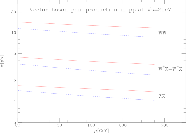
Figure 1: Scale dependence of vector boson pair production cross sections.

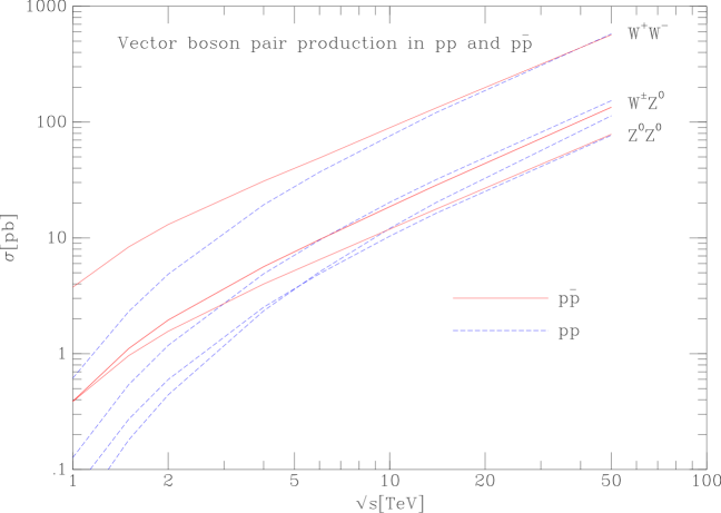
Figure 2: Energy dependence of vector boson pair production cross sections. The scale $\mu$ is taken to be the average vector boson mass.

3 Beyond the zero-width approximation

Part of the reason for re-evaluating the vector boson pair production cross sections is to estimate their importance as backgrounds for new physics processes. In this context the tails of the Breit-Wigner distributions may be important. We are therefore motivated to go beyond the zero width approximation. We consider all standard model contributions to four lepton production, rather than just those proceeding through the production of a pair of vector bosons.

In the zero width approximation $q^{2}=M_{V}^{2}$, the doubly-resonant diagrams form a gauge invariant set. If we wish to move beyond the zero-width approximation, so that we have $q^{2}\neq M_{V}^{2}$, gauge invariance requires that we include all diagrams which contribute to a given final state. This problem has been extensively studied in the $e^{+}e^{-}$ environment where similar diagrams contribute to $W$-pair production [14].

In practice this means that in addition to the diagrams containing two resonant propagators, we must calculate diagrams containing only a single resonant propagator. For the case of $W$-pair production, examples of such doubly and singly resonant diagrams are shown in Figure 3.

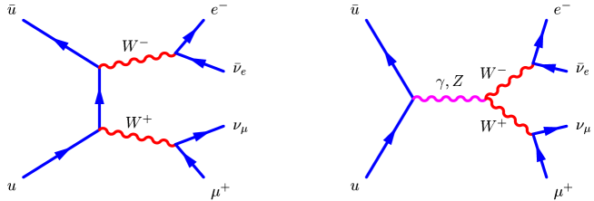
(a)

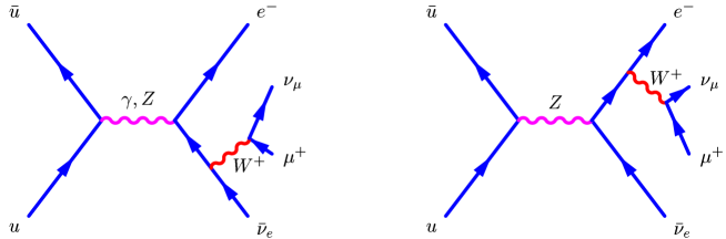
(b)

Figure 3: Doubly (a) and singly (b) resonant diagrams contributing to the parton-level process $q{\bar{q}}\to W^{+}W^{-}\to e^{-}{\bar{\nu}_{e}}\nu_{\mu}\mu^{+}$.

To illustrate the gauge-dependence of the individual sets of diagrams one may work in an axial gauge, taking care to include both the mixed propagators and additional vertices that arise in these gauges.

Even when we include all the diagrams, a second problem arises when we introduce a width for the propagators to avoid on-shell poles. With the modification,

$$\frac{1}{q^{2}-M^{2}}\quad\longrightarrow\quad\frac{1}{q^{2}-M^{2}+iM\Gamma},$$

for each of the propagators, the amplitude is no longer gauge invariant because we now have a mix of singly and doubly resonant diagrams. The Breit-Wigner form of the propagator sums self-energy diagrams which are not separately gauge invariant. Since the resummation of all diagrams which contribute to a given process is not practical, several models have been proposed which allow the introduction of a finite width but preserve gauge invariance.

For a review of the models, the ‘pole-scheme’ [15], the ‘fermion-loop scheme’ [16] and the ‘pinch technique’ [17], see for example Ref. [14]. Here we will adopt the simple prescription whereby we use $1/(q^{2}-M^{2})$ for each propagator initially and then multiply the whole amplitude by,

$$\prod_{\rm props}\,\left(\frac{q^{2}-M^{2}}{q^{2}-M^{2}+iM\Gamma}\right),$$

which clearly maintains gauge invariance [18]. This is the correct treatment for the doubly-resonant piece, but mistreats the singly-resonant diagrams, primarily in the region $q^{2}\sim M^{2}$ where the doubly resonant diagrams dominate. This is the method that we will use to produce our Monte Carlo results in the remainder of this paper. Since the introduction of the width represents an all-orders resummation of an partial set of diagrams, there is no unique way to include it at a given order.

3.1 Cross-sections to leptonic final states

We now present our results for the various leptonic final states using the prescription given above. In practice, the observed cross sections are limited by the acceptance of the detectors in rapidity and in transverse momentum. We quote cross-sections for particular channels with cuts appropriate for Run II and the LHC. Specifically, we apply cuts on the transverse momentum and rapidity of each lepton,

$$p_{T}>20~{}{\rm GeV} \qquad|\eta|<\eta_{\rm max},$$ ,

$$\eta_{\rm max}= \biggl{\{} {2\qquad{\rm Run~{}II}\atop 2.5\qquad{\rm LHC}~{}~{}}$$ (4)

and a cut on the total missing transverse energy,

$$E_{T}/~{}~{}>25~{}{\rm GeV}.$$ (5)

This suffices for $WW$ production; for the other cases we perform a mass cut $75<M_{l^{+}l^{-}}<105~{}{\rm GeV}$. For a more detailed study, one might tailor the cuts individually for each process and include detector resolution effects.

Using the same input as the previous section, but now with the inclusion of the singly-resonant diagrams, our full next-to-leading order results with these cuts are summarized in Tables 5 and 6.

Run II	$W^{-}W^{+}\to e^{-}{\bar{\nu}}e^{+}\nu$		$ZW^{\pm}\to e^{-}e^{+}\bar{\nu}e^{\pm}$		$ZZ\to e^{-}e^{+}\mu^{-}\mu^{+}$		$ZZ\to e^{-}e^{+}(\nu\bar{\nu}\times 3)$
	MRS98	CTEQ5	MRS98	CTEQ5	MRS98	CTEQ5	MRS98	CTEQ5
$\sigma_{\rm cuts}^{\rm NLO}$ [fb]	$70.9$	$73.5$	$2.89$	$2.99$	$1.64$	$1.70$	$10.7$	$11.0$

Table 5: Cross sections (in fb) for various channels at the Tevatron Run II with the cuts of (4) and (5).

LHC	$W^{-}W^{+}\to e^{-}{\bar{\nu}}e^{+}\nu$		$ZW^{+}\to e^{-}e^{+}\nu e^{+}$		$ZW^{-}\to e^{-}e^{+}{\bar{\nu}}e^{-}$		$ZZ\to e^{-}e^{+}\mu^{-}\mu^{+}$
	MRS98	CTEQ5	MRS98	CTEQ5	MRS98	CTEQ5	MRS98	CTEQ5
$\sigma_{\rm cuts}^{\rm NLO}$ [fb]	$514$	$549$	$34.0$	$36.2$	$22.9$	$24.6$	$12.0$	$12.7$

Table 6: Cross sections (in fb) for various channels at the LHC with the cuts of (4) and (5).

4 Examples

In this section we present two examples to demonstrate the use of the $\tt MCFM$ Monte Carlo.

4.1 Tri-lepton production at Run II

One of the ‘gold-plated’ supersymmetry discovery modes at Run II is gaugino pair-production resulting in a tri-lepton signal,

$$p\bar{p}\rightarrow\chi_{1}^{-}(\rightarrow l^{\prime-}\nu\chi_{1}^{0})\,\chi^{0}_{2}(\rightarrow l^{+}l^{-}\chi_{1}^{0}),$$ (6)

where $\chi_{1}^{0}$ is the lightest supersymmetric particle. In order to obtain a clean signal, it is imperative to have a good understanding of the Standard Model background, which is predominantly from leptonic decay of a $WZ$ pair. There have been many previous studies of this background (see [20] and references therein), primarily performed using the ISAJET [21] and PYTHIA [22] event generators. Whilst event generators can have advantages over a fixed order calculation, as presently written ISAJET and PYTHIA do not include the $\gamma^{*}$ contribution or the interference between the photon and the $Z$ in $WZ/\gamma^{*}$ production.

In the recent paper [20], a set of cuts was proposed to further isolate the trilepton signal. However, this study was based on a PYTHIA analysis which includes only the $WZ$ process and not $W\gamma^{*}$ process in assessing the standard model four lepton background.

Following [20], we apply the cuts,

$${\rm central~{}lepton:} p_{T}>11~{}{\rm GeV},\qquad|\eta|<1,$$

$${\rm remaining~{}leptons:} p_{T}>7~{}{\rm GeV~{}and~{}}p_{T}>5~{}{\rm GeV},$$ (7)

$$E_{T}/~{}~{} > 25~{}{\rm GeV},$$

and examine the invariant mass distribution of opposite-sign, same-flavour lepton pairs. This differential cross-section (using the MRS98 structure functions at $\sqrt{s}=2$ TeV) is shown in Figure 4.

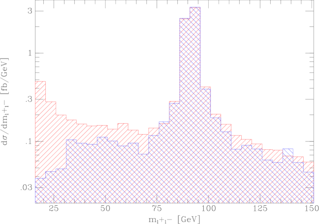
Figure 4: The lepton invariant mass with the full $Z/\gamma^{*}$ interference (single hatched) and with the $Z$ only (double hatched). Each generated event is binned once for each opposite-sign, same-flavour lepton pair. Events which give rise to two entries are binned with half the event weight. The total cross-sections in the plot are $49.4$ fb and $42.6$ fb respectively.

We see that as the invariant mass of deviates from the $Z$-peak, the contribution from the off-shell photon dominates. For the case presented in ref. [20] we have $m_{\chi}\approx 122$ GeV which gives a signal region $10<M_{l^{+}l^{-}}<60$ GeV. Studies using PYTHIA therefore underestimate the standard model background.

4.2 Higgs production via gluon-gluon fusion

At the Tevatron the dominant production mode for a (Standard Model or similar) Higgs boson is via gluon fusion, $gg\to H$ via heavy quark loops. A natural decay mode for $140<M_{H}<180$ GeV is then $H\to W^{(*)}W^{(*)}\to$ leptons/jets, which has been extensively discussed in the literature [23, 24]. The most recent of these studies [24], performed using PYTHIA, optimized a set of cuts to suppress the SM backgrounds for the di-lepton plus missing energy channel and for the like-sign lepton plus jets channel.

Here we perform a parton-level analysis for the di-lepton + missing energy signal. The signal is calculated using the heavy-top effective $ggH$ vertex [25] and we have applied cuts (10)-(16) of [24] which we now describe. In addition to a standard set of cuts,

$$p_{T}(e)>10\ {\rm GeV},\ \ |\eta_{e}|<1.5,$$

$$p_{T}(\mu_{1})>10\ {\rm GeV},\ \ p_{T}(\mu_{2})>5\ {\rm GeV},\ \ |\eta_{\mu}|<1.5,$$

$$m(\ell\ell)>10\ {\rm GeV},\ \ \Delta R(\ell j)>0.4,\ \ \hbox to0.0pt{\hbox to7.95831pt{\hfil/\hfil}\hss}E_{T}>10\ {\rm GeV},$$ (8)

there are further cuts to reduce the various background processes. First we apply,

$$\phi(\ell\ell)<160^{\circ},\ \ \theta(\ell\ell)<160^{\circ}.$$ (9)

where $\phi(\ell\ell)$ is the azimuthal angle in the transverse plane and $\theta(\ell\ell)$ the three-dimensional opening-angle between the two leptons. We also impose,

$$p_{T}(\ell\ell)>20\ {\rm GeV},\ \ \cos\theta_{\ell\ell-\hbox to0.0pt{\hbox to5.57082pt{\hfil/\hfil}\hss}E_{T}}<0.5,\ \ M_{T}(\ell\hbox to0.0pt{\hbox to7.95831pt{\hfil/\hfil}\hss}E_{T})>20\ {\rm GeV},$$ (10)

where $\theta_{\ell\ell-\hbox to0.0pt{\hbox to5.57082pt{\hfil/\hfil}\hss}E_{T}}$ is the relative angle between the lepton pair transverse momentum and the missing transverse momentum and the two-body transverse-mass is defined for each lepton and the missing energy as,

$$M_{T}^{2}(\ell\hbox to0.0pt{\hbox to7.95831pt{\hfil/\hfil}\hss}E_{T})=2p_{T}(\ell)\hbox to0.0pt{\hbox to7.95831pt{\hfil/\hfil}\hss}E_{T}(1-\cos\theta_{\ell-\hbox to0.0pt{\hbox to5.57082pt{\hfil/\hfil}\hss}E_{T}}).$$ (11)

Further di-lepton mass cuts are,

$$m(\ell\ell) < 78\ {\rm GeV}\ \ {\rm for}\ e^{+}e^{-},\mu^{+}\mu^{-},$$

$$m(\ell\ell) < 110\ {\rm GeV}\ \ {\rm for}\ e\mu,$$ (12)

and we also cut on the Dittmar-Dreiner angle $\theta^{*}_{\ell_{1}}$ for each lepton $\ell_{1}$,

$$-0.3<\cos\theta^{*}_{\ell_{1}}<0.8.$$ (13)

Finally, we introduce a jet veto,

$${\rm veto\ if}\ \ p_{T}^{j_{1}}>95\ {\rm GeV},\ \ |\eta_{j}|<3,$$

$${\rm veto\ if}\ \ p_{T}^{j_{2}}>50\ {\rm GeV},\ \ |\eta_{j}|<3,$$ (14)

and reject events where either jet is $b$-tagged with an efficiency,

$$\epsilon_{b}=1.1\times 57\%\ {\rm tanh}({\eta_{b}\over 36.05}).$$ (15)

The results of our analysis ($\sigma_{\rm cuts}$) at $\sqrt{s}=2$ TeV for $140<m_{H}<190$ are shown in Table 7, where we have employed the structure function set MRS98. Also shown in Table 7 are the total cross sections for the various channels which serve as normalizations of our results. The primary background in this channel is from $W^{+}W^{-}$ with smaller backgrounds from top pair production, $WZ$ and $ZZ$ production. For the signal, we choose the renormalization scale $\mu=m_{H}$; for the di-boson backgrounds we again use the mean boson mass. In the case of the $t{\bar{t}}$ background we set $\mu=100$ GeV; order $\alpha_{s}^{3}$ corrections to the total top pair production cross-section are small at this scale [26].

Our analysis confirms that the $WW$ process is the principal background for Higgs production in the region $140<m_{H}<190$. Note that we have not included the decay $W(\rightarrow\tau\nu\rightarrow l+X)$ in our calculations. The comparison with ref. [24] (where these effects are included) is therefore not exact. The effects of $\tau$ decays are stated to be small in ref. [24].

We find that all the backgrounds due to the di-boson processes are larger than in ref. [24], primarily because we have normalized to the $O(\alpha_{s})$ cross-sections which are about $30\%$ bigger than the Born cross-sections, (c.f. Table 3). Note however that our signal cross sections are also larger than Ref. [24] by about $20\%$, so the net effect on $S/\sqrt{B}$ may be small. In addition, we find that the background from the $WZ$-class of events is about twice as big as ref. [24] because of our inclusion of the $W\gamma^{*}$ contribution, which was left out in ref. [24]. Our estimate of the $t\bar{t}$ background is smaller than in Ref. [24], perhaps because we do not include leptons from $b$-decay.

Signal ($m_{H}$)	140	150		160	170	180		190
$\sigma_{\rm cuts}$ (fb)	$4.36$	$5.32$		$6.12$	$5.15$	$3.90$		$2.47$
$\sigma_{\rm total}$ (pb)	$0.181$	$0.206$		$0.215$	$0.180$	$0.143$		$0.0976$
Background	$WW$		$t{\bar{t}}$		$ZZ$		$WZ$
$\sigma_{\rm cuts}$ (fb)	$185$		$9.55$		$2.48$		$10.4$
$\sigma_{\rm total}$ (pb)	$13.0$		$6.82$		$1.56$		$3.96$

Table 7: Signal and background cross-sections for a Higgs search with di-lepton final states. The $\tau^{+}\tau^{-}$ background is negligible with these cuts. For comparison, the total cross sections (without leptonic decays from the vector bosons) are also shown.

5 Conclusions

We have presented a Monte Carlo program for vector-boson pair production at hadron colliders, including for the first time the complete ${\cal O}(\alpha_{s})$ corrections with leptonic decay correlations.

We have employed this program to calculate the total di-boson cross-sections, first as a cross-check with existing results in the literature and secondly in order to provide an update of predictions for Run II at the Tevatron and for the LHC, including the latest structure functions and strong coupling. The cross sections are larger than previous estimates in the literature.

The advantage of this Monte Carlo is only realized when cuts are applied to the final-state leptons. This is primarily of importance when estimating Standard Model backgrounds to new physics, which is especially crucial at the Tevatron. For this reason we have provided two examples of such uses in Run II, tri-lepton production as a SUSY signal and a di-lepton analysis for an intermediate-mass Higgs search.

Appendix A Appendix: Amplitudes for four fermion processes

We first introduce a separation of the total $n$-particle tree-level amplitude into its doubly- and singly-resonant components,

$${\cal A}_{n}^{\rm tree}={\cal C}^{\rm coup}\left({\cal A}_{n,{\rm DR}}^{\rm tree}+{\cal A}_{n,{\rm SR}}^{\rm tree}\right),$$ (16)

where ${\cal C}^{\rm coup}$ is an overall coupling factor depending on the di-boson process under consideration. The contributions ${\cal A}_{n,{\rm DR}}^{\rm tree}$ were first calculated in [19] although we will closely follow the more recent notation and approach of [1]. In particular, the amplitudes are presented in terms of particle momenta $p_{i}$ that are all outgoing, so that momentum conservation implies $\sum_{i}p_{i}=0$.

A.1 $W^{+}W^{-}$ final states

For this process we label the particles as,

$$0\to q_{1}{\bar{q}}_{2}\,W^{-}\left(\to\ell_{3}{\bar{\nu}}_{4}\right)\,W^{+}\left(\to{\bar{\ell}}_{5}\nu_{6}\right),$$

where the leptons are not necessarily of the same flavour, and we write the process in this manner to remind the reader that $q_{1}$ represents an outgoing quark (so that when we cross to obtain the desired result, it becomes an incoming anti-quark). Then from [1] we see that the non-vanishing doubly-resonant helicity amplitudes for up-quark annihilation are (with labels suppressed where possible),

$${\cal A}_{6,{\rm DR}}^{\rm tree}(u_{1}^{L},{\bar{u}}_{2}^{R}) = \left(A_{6}^{{\rm tree},a}(1,2,3,4,5,6)+C_{L,u}A_{6}^{{\rm tree},b}(1,2,3,4,5,6)\right){\cal P}_{34}{\cal P}_{56},$$

$${\cal A}_{6,{\rm DR}}^{\rm tree}(u_{1}^{R},{\bar{u}}_{2}^{L}) = C_{R,u}A_{6}^{{\rm tree},b}(2,1,3,4,5,6)\,{\cal P}_{34}{\cal P}_{56},$$ (17)

with the sub-amplitudes $A_{6}^{{\rm tree}}$ given by equations (2.8) and (2.9) of [1]. The ${\cal P}_{ij}$ are propagator factors given by,

$${\cal P}_{ij}=\frac{s_{ij}}{s_{ij}-M_{ij}^{2}},$$ (18)

with $M_{12}=M_{Z}$ and $M_{34}=M_{56}=M_{W}$. The couplings that appear in these amplitudes are,

$${\cal C}^{\rm coup} = \left(\frac{e^{2}}{\sin^{2}\theta_{W}}\right)^{2},$$ (19)

$$C_{L,\{{u\atop d}\}} = \pm 2Q_{\{{u\atop d}\}}\sin^{2}\theta_{W}+(1\mp 2Q_{\{{u\atop d}\}}\sin^{2}\theta_{W}){\cal P}_{12},$$ (20)

$$C_{R,\{{u\atop d}\}} = \pm 2Q_{\{{u\atop d}\}}\sin^{2}\theta_{W}\left(1-{\cal P}_{12}\right),$$ (21)

where $Q_{i}$ is the electric charge in units of the positron charge. For the additional singly-resonant diagrams we find,

$${\cal A}_{6,{\rm SR}}^{\rm tree}(u_{1}^{L},{\bar{u}}_{2}^{R})=2\sin^{2}\theta_{W}\times\Bigl{\{}$$

$$\left({\cal P}_{56}A_{6}^{{\rm tree},a}(3,4,6,5,2,1)+{\cal P}_{34}A_{6}^{{\rm tree},a}(6,5,1,2,4,3)\right)v_{L,n}v_{L,u}{\cal P}_{12}$$

$$+ \left({\cal P}_{56}A_{6}^{{\rm tree},a}(3,4,1,2,5,6)+{\cal P}_{34}A_{6}^{{\rm tree},a}(6,5,3,4,2,1)\right)\left(Q_{u}Q_{e}+v_{L,e}v_{L,u}{\cal P}_{12}\right)\Bigr{\}},$$

$${\cal A}_{6,{\rm SR}}^{\rm tree}(u_{R},{\bar{u}}_{L})={\cal A}_{6,{\rm SR}}^{\rm tree}(u_{L},{\bar{u}}_{R})\left(L\leftrightarrow R,1\leftrightarrow 2\right),$$ (22)

where we have introduced a further set of scaled couplings [1],

$$v_{L,e}={-1-2Q_{e}\sin^{2}\theta_{W}\over\sin 2\theta_{W}}, \qquad v_{R,e}=-{2Q_{e}\sin^{2}\theta_{W}\over\sin 2\theta_{W}},$$ (23)

$$v_{L,q}={\pm 1-2Q_{q}\sin^{2}\theta_{W}\over\sin 2\theta_{W}}, \qquad v_{R,q}=-{2Q_{q}\sin^{2}\theta_{W}\over\sin 2\theta_{W}},$$ (24)

$$v_{L,n}={1\over\sin 2\theta_{W}}.$$ (25)

Note that here the sub-amplitudes needed for the singly-resonant diagrams are exactly those introduced in [1] to describe the doubly-resonant diagrams. This is because the diagrams are topologically equivalent and (modulo couplings) we can obtain the singly resonant amplitudes by simply re-labelling the external legs. The down-quark amplitudes may be obtained simply by symmetry,

$${\cal A}_{6,{\rm DR}}^{\rm tree}(d,{\bar{d}}) = {\cal A}_{6,{\rm DR}}^{\rm tree}(u,{\bar{u}})\left(u\leftrightarrow d,3\leftrightarrow 6,4\leftrightarrow 5\right),$$

$${\cal A}_{6,{\rm SR}}^{\rm tree}(d,{\bar{d}}) = {\cal A}_{6,{\rm SR}}^{\rm tree}(u,{\bar{u}})\left(u\leftrightarrow d\right).$$ (26)

As described in [1], the doubly-resonant amplitudes for the process with an additional gluon radiated from the quark line are exactly analogous to (17) and require the introduction of functions ${\cal A}_{7,{\rm tree}}$. However, unlike the 6-particle amplitudes, these functions are not sufficient to describe the singly-resonant diagrams. In this case, initial state gluon radiation in the singly-resonant diagrams would correspond to final-state radiation in the equivalent doubly-resonant diagrams and thus we need to introduce a new set of sub-amplitudes. For a positive helicity gluon of momentum $p_{7}$ we find,

$${\cal A}_{7,{\rm SR}}^{\rm tree}(u^{L}_{1},{\bar{u}}^{R}_{2},g_{7}^{+})=2\sin^{2}\theta_{W}\times\Bigl{\{}$$

$$\left({\cal P}_{56}B_{7}^{{\rm tree},a}(1,2,3,4,5,6,7)+{\cal P}_{34}B_{7}^{{\rm tree},b}(2,1,3,4,5,6,7)\right)v_{L,n}v_{L,u}{\cal P}_{127}$$

$$+ \left({\cal P}_{56}B_{7}^{{\rm tree},b}(2,1,6,5,4,3,7)+{\cal P}_{34}B_{7}^{{\rm tree},a}(1,2,6,5,4,3,7)\right)\left(Q_{u}Q_{e}+v_{L,e}v_{L,u}{\cal P}_{127}\right)\Bigr{\}},$$

where the new functions are defined by,

$$B_{7}^{{\rm tree},a} = {i\,\left\langle 3\hskip 0.42677pt6\right\rangle\langle\mskip-1.0mu{1}|(2+7)|{4}\mskip-1.0mu\rangle\langle\mskip-1.0mu{1}|(3+6)|{5}\mskip-1.0mu\rangle\over{\left\langle 1\hskip 0.42677pt7\right\rangle\left\langle 2\hskip 0.42677pt7\right\rangle s_{56}\;t_{127}\ t_{356}}},$$ (28)

and,

$$B_{7}^{{\rm tree},b} = {-i\,\left\langle 2\hskip 0.42677pt6\right\rangle\left[4\hskip 0.42677pt5\right]\left[\left\langle 1\hskip 0.42677pt2\right\rangle\langle\mskip-1.0mu{3}|(5+4)|{1}\mskip-1.0mu\rangle-\left\langle 2\hskip 0.42677pt7\right\rangle\langle\mskip-1.0mu{3}|(5+4)|{7}\mskip-1.0mu\rangle\right]\over{\left\langle 1\hskip 0.42677pt7\right\rangle\left\langle 2\hskip 0.42677pt7\right\rangle s_{34}t_{127}t_{345}}}.$$ (29)

Our definition of the spinor products follows ref. [1]. The remaining amplitudes are obtained as above, with the additional (negative helicity) gluon corresponding, as in the doubly-resonant case, to the operation $-{\rm flip}_{1}$ defined in [1]. As will be the case for all the amplitudes in this appendix, the loop contributions for the singly-resonant diagrams may be simply obtained by following the prescription (3.20) of [1].

A.2 $W^{\pm}Z$ final states

Here we label the two processes slightly differently,

$$0 \to q_{1}{\bar{q}}_{2}\,W^{-}\left(\to\ell_{3}{\bar{\nu}}_{4}\right)\,Z\left(\to{\bar{\ell}}_{5}\ell_{6}\right),$$

$$0 \to q_{1}{\bar{q}}_{2}\,W^{+}\left(\to\nu_{3}{\bar{\ell}}_{4}\right)\,Z\left(\to{\bar{\ell}}_{5}\ell_{6}\right),$$ (30)

in order to simplify the form of the amplitudes and the overall coupling (c.f. ref. 16) is,

$${\cal C}^{\rm coup}=\left(\frac{e^{2}}{\sin\theta_{W}}\right)^{2}.\\$$

The doubly-resonant amplitude for a left-handed decay of the $Z$ is,

$${\cal A}_{6,{\rm DR}}^{\rm tree}(q_{1},{\bar{q}}_{2},\ell_{6}^{L}) = A_{6}^{{\rm tree},a}(1,2,3,4,5,6)\left(v_{L,q_{2}}v_{L,e}{\cal P}_{56}+Q_{q_{2}}Q_{e}\right){\cal P}_{34}$$ (31)

$$+ A_{6}^{{\rm tree},a}(1,2,6,5,4,3)\left(v_{L,q_{1}}v_{L,e}{\cal P}_{56}+Q_{q_{1}}Q_{e}\right){\cal P}_{34}$$

$$\pm A_{6}^{{\rm tree},b}(1,2,3,4,5,6)\left(v_{L,e}\cot\theta_{W}{\cal P}_{56}+Q_{e}\right){\cal P}_{12}{\cal P}_{34},$$

where the masses in the propagators are now $M_{12}=M_{34}=M_{W}$ and $M_{56}=M_{Z}$. For $W^{+}$ production we have $q_{1}=d$, $q_{2}=u$ and the third line has a positive contribution, whilst $W^{-}$ corresponds to $q_{1}=u$, $q_{2}=d$ and a negative sign. This reduces to the form given in [1] if we set $Q_{e}=0$ to neglect the virtual photon diagrams. The right-handed amplitude is obtained by a symmetry transformation,

$${\cal A}_{6,{\rm DR}}^{\rm tree}(q_{1},{\bar{q}}_{2},\ell_{6}^{R})={\cal A}_{6,{\rm DR}}^{\rm tree}(q_{1},{\bar{q}}_{2},\ell_{6}^{L})\left(v_{L,e}\leftrightarrow v_{R,e},5\leftrightarrow 6\right).$$ (32)

The singly resonant diagrams are somewhat more complicated. With a $Z$ propagator we can couple both electrons and neutrinos, while $\gamma^{*}$ may only couple directly to the electrons. In addition, if the final state electrons are both left-handed, there is a contribution from a diagram containing two $W$ propagators. In total we obtain,

$${\cal A}_{6,{\rm SR}}^{\rm tree}(q_{1},{\bar{q}}_{2},\ell_{6}^{L}) = \left(v_{L,1}A_{6}^{{\rm tree},a}(3,4,6,5,2,1)+v_{L,2}A_{6}^{{\rm tree},a}(3,4,1,2,5,6)\right){\cal P}_{56}{\cal P}_{12}v_{L,e}$$ (33)

$$+ \left(c_{1}A_{6}^{{\rm tree},a}(3,4,6,5,2,1)+c_{2}A_{6}^{{\rm tree},a}(3,4,1,2,5,6)\right){\cal P}_{12}Q_{e}^{2}$$

$$+ \left(c_{1}A_{6}^{{\rm tree},a}(6,5,1,2,4,3)+c_{2}A_{6}^{{\rm tree},a}(6,5,3,4,2,1)\right)\frac{{\cal P}_{12}{\cal P}_{34}}{2\sin^{2}\theta_{W}},$$

where the newly introduced couplings $v_{L,i}$ and $c_{i}$ depend upon the process under consideration and are given by,

$$W^{+} : c_{1}=0,\qquad c_{2}=1,\qquad v_{L,1}=v_{L,n},\qquad v_{L,2}=v_{L,e},$$

$$W^{-} : c_{1}=1,\qquad c_{2}=0,\qquad v_{L,1}=v_{L,e},\qquad v_{L,2}=v_{L,n}.$$ (34)

The right-handed contribution is similar, but does not contain the corresponding final term,

$${\cal A}_{6,{\rm SR}}^{\rm tree}(q_{1},{\bar{q}}_{2},\ell_{6}^{R}) = \left(v_{L,1}A_{6}^{{\rm tree},a}(3,4,5,6,2,1)+v_{L,2}A_{6}^{{\rm tree},a}(3,4,1,2,6,5)\right){\cal P}_{56}{\cal P}_{12}v_{R,e}$$ (35)

$$+ \left(c_{1}A_{6}^{{\rm tree},a}(3,4,5,6,2,1)+c_{2}A_{6}^{{\rm tree},a}(3,4,1,2,6,5)\right){\cal P}_{12}Q_{e}^{2}.$$

We now turn to the graphs including gluon radiation. For the doubly resonant contribution with a positive helicity gluon we find a similar structure,

$${\cal A}_{7,{\rm DR}}^{\rm tree}(q_{1},{\bar{q}}_{2},\ell_{6}^{L},g_{7}^{+}) = A_{7}^{{\rm tree},a}(1,2,3,4,5,6,7)\left(v_{L,q_{2}}v_{L,e}{\cal P}_{56}+Q_{q_{2}}Q_{e}\right){\cal P}_{34}$$ (36)

$$+ A_{7}^{{\rm tree},a}(1,2,6,5,4,3,7)\left(v_{L,q_{1}}v_{L,e}{\cal P}_{56}+Q_{q_{1}}Q_{e}\right){\cal P}_{34}$$

$$\pm A_{7}^{{\rm tree},b}(1,2,3,4,5,6,7)\left(v_{L,e}\cot\theta_{W}{\cal P}_{56}+Q_{e}\right){\cal P}_{127}{\cal P}_{34},$$

whilst the singly resonant pieces again require the new amplitudes,

$${\cal A}_{7,{\rm SR}}^{\rm tree}(q_{1},{\bar{q}}_{2},\ell_{6}^{L},g_{7}^{+}) = \left(v_{L,1}B_{7}^{{\rm tree},a}(1,2,3,4,5,6,7)+v_{L,2}B_{7}^{{\rm tree},b}(2,1,6,5,4,3,7)\right){\cal P}_{56}{\cal P}_{127}v_{L,e}$$ (37)

$$+ \left(c_{1}B_{7}^{{\rm tree},a}(1,2,3,4,5,6,7)+c_{2}B_{7}^{{\rm tree},b}(2,1,6,5,4,3,7)\right){\cal P}_{127}Q_{e}^{2}$$

$$+ \left(c_{1}B_{7}^{{\rm tree},b}(2,1,3,4,5,6,7)+c_{2}B_{7}^{{\rm tree},a}(1,2,6,5,4,3,7)\right)\frac{{\cal P}_{127}{\cal P}_{34}}{2\sin^{2}\theta_{W}},$$

$${\cal A}_{7,{\rm SR}}^{\rm tree}(q_{1},{\bar{q}}_{2},\ell_{6}^{R},g_{7}^{+}) = \left(v_{L,1}B_{7}^{{\rm tree},a}(1,2,3,4,6,5,7)+v_{L,2}B_{7}^{{\rm tree},b}(2,1,5,6,4,3,7)\right){\cal P}_{56}{\cal P}_{127}v_{R,e}$$ (38)

$$+ \left(c_{1}B_{7}^{{\rm tree},a}(1,2,3,4,6,5,7)+c_{2}B_{7}^{{\rm tree},b}(2,1,5,6,4,3,7)\right){\cal P}_{127}Q_{e}^{2}.$$

The remaining amplitudes, with the helicity of the gluon reversed, can be obtained by the transformation,

$${\cal A}_{7,{\rm SR}}^{\rm tree}(q_{1},{\bar{q}}_{2},\ell_{6},g_{7}^{-})=-{\cal A}_{7,{\rm SR}}^{\rm tree}(q_{1},{\bar{q}}_{2},\ell_{6},g_{7}^{+})\left(4\leftrightarrow 6,3\leftrightarrow 5,\langle ab\rangle\leftrightarrow[ab],B_{7}^{{\rm tree},a}\leftrightarrow B_{7}^{{\rm tree},b}\right).$$ (39)

References

- [1] L. Dixon, Z. Kunszt and A. Signer, Nucl. Phys. B531 (1998) 3.
- [2] B. Mele, P. Nason and G. Ridolfi, Nucl. Phys. B357 (1991) 409.
- [3] S. Frixione, P. Nason and G. Ridolfi, Nucl. Phys. B383 (1992) 3.
- [4] S. Frixione, Nucl. Phys. B410 (1993) 280.
- [5] J. Ohnemus and J. F. Owens, Phys. Rev. D43 (1991) 3626.
-
[6]
J. Ohnemus, Phys. Rev. D44 (1991) 1403;
J. Ohnemus, Phys. Rev. D44 (1991) 3477. - [7] J. Ohnemus, Phys. Rev. D50 (1994) 1931.
- [8] S. Catani and M.H. Seymour, Nucl.Phys. B485 (1997) 291 Erratum-ibid. B510(1997) 503.
- [9] R.K. Ellis, D.A. Ross, A.E. Terrano, Nucl.Phys. B178 (1981) 421.
- [10] A. D. Martin, R. G. Roberts, W. J. Stirling, R. S. Thorne, Eur. Phys. J. C4 (1998) 463.
- [11] CTEQ collaboration, H. L. Lai et al., MSU-HEP-903100, hep-ph/9903282.
- [12] P. N. Harriman, A. D. Martin, R. G. Roberts and W. J. Stirling, Phys. Rev. D42 (1990) 798.
- [13] C. Caso et al., Eur. Phys. J. C3 (1998) 1.
- [14] ‘WW cross-sections and distributions’, in Physics at LEP 2, vol. 1, ed. G. Altarelli, T. Sjöstrand and F. Zwirner, CERN Yellow Report 96-01.
-
[15]
M. Veltman, Physica 29 (1963) 186;
R. G. Stuart, Phys. Lett. B262 (1991) 113;
A. Aeppli, G. J. van Oldenborgh and D. Wyler, Nucl. Phys. B428 (1994) 126. -
[16]
U. Baur and D. Zeppenfeld, Phys. Rev. Lett. 75 (1995) 1002;
C. G. Papadopoulos, Phys. Lett. B352 (1995) 144;
E. N. Argyres et al., Phys. Lett. B358 (1995) 339. - [17] J. Papavassiliou and A. Pilaftsis, Phys. Rev. D53 (1996) 2128.
-
[18]
U. Baur, J. A. M. Vermaseren and D. Zeppenfeld, Nucl. Phys. B375 (1992) 3;
Y. Kurihara, D. Perret-Gallix and Y. Shimizu, Phys. Lett. B349 (1995) 367. - [19] J. F. Gunion and Z. Kunszt, Phys. Rev. D33 (1986) 665.
- [20] K. T. Matchev and D. M. Pierce, FERMILAB-PUB-99/078-T, hep-ph/9904282.
- [21] F.E. Paige and S.D. Protopopescu, in Proc. UCLA Workshop, eds. H.-U. Bengtsson et al., World Scientific, Singapore (1986).
-
[22]
H.-U. Bengtsson and T. Sjöstrand,
Comp. Phys. Comm. 46 (1987) 43
T. Sjöstrand, Comp. Phys. Comm. 82 (1994) 74. -
[23]
E. W. N.. Glover, J. Ohnemus and S. S. D. Willenbrock, Phys. Rev. D37
(1988) 3193;
V. Barger, G. Bhattacharya, T. Han and B. A. Kniehl, Phys. Rev. D43 (1991) 779;
J. Gunion and T. Han, Phys. Rev. D51 (1995) 1051;
M. Dittmar and H. Dreiner, Phys. Rev. D55 (1997) 167;
T. Han and R.-J. Zhang, Phys. Rev. Lett. 82 (1999) 25. - [24] T. Han, A. S. Turcot and R.-J. Zhang, Phys. Rev. D59 (1999) 093001.
-
[25]
S. Dawson, Nucl. Phys. B359 (1991) 283;
A. Djouadi, M. Spira, P.M. Zerwas, Phys. Lett. B264 (1991) 440. - [26] see, for example, R.K. Ellis, W.J. Stirling and B.R. Webber, QCD and Collider Physics, Cambridge University Press, (1996).