On Multiphoton Bremsstrahlung

Abstract

Kinetic equations for the process of multiphoton bremsstrahlung of electron in a matter have been used to derive the equations for the moments of distributions of electrons over the number of emitted photons and over the energy loss. The equations for the moments have been solved in continuous slowing down approximation. It has been shown that the moments of multiphoton distributions can be expressed in terms of the moments of macroscopic differential cross section of the process. The results of analytical calculations have been compared with the data of Monte Carlo simulation.

Tomsk Polytechnic University, 634034, Tomsk, Russia

1 Introduction

The bremsstrahlung of electrons passing through a matter is an example of stochastic process where the number of emitted photons as well as their energies are random. The importance of multiphoton effects was underlined in [1] where the problems of experimental study of bremsstrahlung cross section were discussed. The summary energy of emitted photons, as a rule, is measured in such experiments and the distribution of electrons over energy loss differs from the energy distribution of radiated photons [2]. Kinetic equations for the distribution of electrons over the number of emitted photons and for the distribution over the radiation energy loss are given in the paper. They are used to get the equations for the moments of the distributions. Qualitative analysis of the path and energy dependences of the moments is given in continuous slowing down approximation with simple relativistic Bethe-Heitler formula for the macroscopic differential cross section of bremsstrahlung. It is shown that the moments of differential cross section can be expressed in terms of the moments of energy loss distribution which can be determined in experimental way. The results of the analysis are compared with the data of Monte Carlo simulation.

2 Kinetic equations for multiphoton bremsstrahlung

Let us consider an electron of energy $E$ traveling in a matter the path length $l$. The probability $P(n|E,l)$ to emit $n$ photons of bremsstrahlung along the pass $l$ obeys the balance equation (the Kolmogorov-Chapman equation) [3]:

$$P(n|E,l)=(1-s\Sigma(E))P(n|E,l-s)+s\Sigma(E)\int_{0}^{E}\frac{\Sigma(E_{\gamma};E)}{\Sigma(E)}P(n-1|E-E_{\gamma},l)dE_{\gamma},$$ (1)

$\Sigma(E)$ and $\Sigma(E_{\gamma};E$$)$ being the total and differential macroscopic cross sections of bremsstrahlung, $s$ is a small part of $l$ . The first term in the right side of Eq.(1) corresponds to electrons which pass small path $s$ without radiation and $1-s\Sigma(E)$ is corresponding probability. These electrons have to emit $n$ photons along the rest of the path $l-s.$ The second term corresponds to the electrons which emit the first photon passing path $s$ and $s\Sigma(E)$ is corresponding probability. These electrons have to emit $n-1$ photons after that but the energy of electrons equals to $E-E_{\gamma}$ where $E_{\gamma}$ is random energy of the first emitted photon and $\Sigma(E_{\gamma};E)/\Sigma(E)$ is the probability density function of $E_{\gamma}$ . In the limit $s\rightarrow 0$ the formula (1) gives the integro-differential equation for $P(n|E,l)$ [4]:

$$\frac{\partial}{\partial l}P(n|E,l)+\Sigma(E)P(n|E,l)-\int^{E}_{0}\Sigma(E_{\gamma};E)P(n-1|E-E_{\gamma},l)dE_{\gamma}$$ (2)

with boundary condition

$$P(n|E,l=0)=\delta_{no.}$$

In similar way one can obtain the balance equation for the probability density function $P(Q|E,l)$ describing the distribution of electrons over the energy loss $Q$ :

$$P(Q|E,l)=(1-s\Sigma(E))P(Q|E,l-s)+s\Sigma(E)\int_{0}^{E}\frac{\Sigma(E_{\gamma};E)}{\Sigma(E)}P(Q-E_{\gamma}|E-E_{\gamma},l)dE_{\gamma},$$

which leads to the equation [4]

$$\frac{\partial}{\partial l}P(Q|E,l)+\Sigma(E)P(Q|E,l)-\int^{E}_{0}\Sigma(E_{\gamma};E)P(Q-E_{\gamma}|E-E_{\gamma},l)dE_{\gamma}$$ (3)

with boundary condition

$$P(Q|E,l=0)=\delta(Q),$$

$\delta(Q)$ being the Dirac $\delta$ -function.

Multiplication of both side of Eq.(3) by $Q^{n}$ and integration over $Q$ gives the equations for the moments of the distribution $P(Q|E,l):$

$$\overline{Q^{n}}(E,l)=\int^{E}_{0}Q^{n}P(Q|E,l)dQ.$$

The equations for two first moments have the form [4]:

$$\frac{\partial}{\partial l}\overline{Q}(E,l)+\Sigma(E)\overline{Q}(E,l)-\int^{E}_{0}\Sigma(E_{\gamma};E)\overline{Q}(E-E_{\gamma},l)dE_{\gamma}=\beta(E),$$ (4)

$$\overline{Q}(E,l=0)=0,$$

$$\frac{\partial}{\partial l}\overline{Q^{2}}(E,l)+\Sigma(E)\overline{Q^{2}}(E,l)-\int^{E}_{0}\Sigma(E_{\gamma};E)\overline{Q^{2}}(E-E_{\gamma},l)dE_{\gamma}=\gamma(E)+2\int^{E}_{0}E_{\gamma}\Sigma(E_{\gamma};E)\overline{Q}(E-E_{\gamma},l)dE_{\gamma},$$ (5)

$$\overline{Q^{2}}(E,l=0)=0.$$

Quantities $\beta(E)$ and $\gamma(E)$ in (4) and (5) are the moments of differential cross section $\Sigma(Q;E):$

$$\beta(E)=\int_{0}^{E}E_{\gamma}\Sigma(E_{\gamma};E)dE_{\gamma},$$

$$\gamma(E)=\int_{0}^{E}E_{\gamma}^{2}\Sigma(E_{\gamma};E)dE_{\gamma}.$$

3 Continuous slowing down approximation

If differential cross section $\Sigma(E_{\gamma};E)$ is rapidly decreasing function of the variable $E_{\gamma}$ the collision integrals in (2), (4), (5) can be transformed by the Taylor expansion of integrands:

$$P(n-1|E-E_{\gamma},l)\approx P(n-1|E,l)-E_{\gamma}\frac{\partial}{\partial E}P(n-1|E,l),$$

$$\overline{Q}(E-E_{\gamma},l)\approx\overline{Q}(E,l)-E_{\gamma}\frac{\partial}{\partial E}\overline{Q}(E,l),$$

$$\overline{Q^{2}}(E-E_{\gamma},l)\approx\overline{Q^{2}}(E,l)-E_{\gamma}\frac{\partial}{\partial E}\overline{Q^{2}}(E,l).$$

Such transform leads to the equations:

$$\frac{\partial}{\partial l}P(n|E,l)+\Sigma(E)P(n|E,l)=\Sigma(E)P(n-1|E,l)-\beta(E)\frac{\partial}{\partial E}P(n-1|E,l),$$ (6)

$$\frac{\partial}{\partial l}\overline{Q}(E,l)+\beta(E)\frac{\partial}{\partial E}\overline{Q}(E,l)=\beta(E),$$ (7)

$$\frac{\partial}{\partial l}\overline{Q^{2}}(E,l)+\beta(E)\frac{\partial}{\partial E}\overline{Q^{2}}(E,l)=\gamma(E)+2\beta(E)\overline{Q}(E,l)-2\gamma(E)\frac{\partial}{\partial E}\overline{Q}(E,l).$$ (8)

It follows from the Eq.(6) that in $\Sigma(E)\approx const$ approximation $P(n|E,l)$ is the Poisson distribution:

$$P(n|E,l)=\exp(-l\Sigma(E))\frac{(l\Sigma(E))^{n}}{n!}$$ (9)

with the mean number (multiplicity) of emitted photons equals to

$$\overline{n}(E,l)=\Sigma^{\infty}_{n=0}nP(n|E,l)=l\Sigma(E).$$ (10)

To get the solutions of (7), (8) quantities $\beta(E)$ and $\gamma(E)$ have to be determined.

4 Numerical data for bremsstrahlung

For a qualitative analysis of the multiphoton bremsstrahlung we used the simplified relativistic Bethe-Heitler formula [2] for the differential cross section:

$$\Sigma(E_{\gamma};E)=\frac{1}{tE_{\gamma}}(\frac{4}{3}(1-\frac{E_{\gamma}}{E})+\frac{E_{\gamma}^{2}}{E^{2}}),(E^{(c)}_{\gamma}\leq E_{\gamma}\leq E),$$ (11)

where $t$ is the radiation length of the material passed by electron and $E_{\gamma}^{(c)}=\alpha E$ is the cut off energy. The cut of for the bremsstrahlung photon spectra is due to the density effect [5] which suppresses significantly the soft part of the spectrum. Parameter $\alpha$ can be estimated by the formula

$$\alpha\sim\frac{\hbar\omega_{p}}{mc^{2}},$$

where $\hbar\omega_{p}$ is the plasmon energy of the target material, $mc^{2}=511$ keV is the rest energy of an electron.

Such $\Sigma(E_{\gamma};E)$ leads to the energy independent cross section

$$\Sigma(E)\approx\frac{1}{t}(\frac{4}{3}\ln\frac{1}{\alpha}-\frac{5}{6})$$ (12)

and to the approximate formulas for $\beta$ and $\gamma:$

$$\beta(E)\approx\frac{E}{t},$$

$$\gamma(E)\approx\frac{E^{2}}{2t}.$$

One can see from (10), (12) that the photon multiplicity $\overline{n}$ doesn’t depend on the electron energy and is determined by the target thickness only.

Substitution of approximate expression for $\beta$ and $\gamma$ into (7), (8) and solution of these equations gives the formulas for the moments:

$$\overline{Q}(E,l)=E(1-\exp(-\frac{l}{t})),$$ (13)

$$\overline{Q^{2}}(E,l)=\frac{E^{2}}{4}(3-4\exp(-\frac{l}{t})+\exp(-\frac{2l}{t}))$$

and for the variance:

$$\sigma_{Q}^{2}(E,l)=\overline{Q^{2}}(E,l)-\overline{Q}^{2}(E,l)=\frac{E^{2}}{4}(4\exp(-\frac{l}{t})-3\exp(-\frac{2l}{t})-1).$$ (14)

It is seen from (13), (14), that for $\frac{l}{t}\ll 1$ the moments of bremsstrahlung differential cross section $\beta$ and $\gamma$ can be expressed in terms of the moments of the energy loss distribution $\overline{Q}$ and $\sigma_{Q}^{2}$ $:$

$$\overline{Q}(E,l)\approx l\frac{E}{t}=l\beta(E),$$

$$\sigma_{Q}^{2}\approx l\frac{E^{2}}{2t}=l\gamma(E),$$

which can be determined in experiments where the characteristics of energy loss distribution are measured.

Formulas (10), (13) and (14) were used to calculate $\overline{n,}$ $\overline{Q}$ and $\sigma_{Q}^{2}$ for 8 GeV electron bremsstrahlung in tungsten target. The results were compared with the data of Monte Carlo simulation using the GEANT code [6]. The Monte Carlo method was used for calculation of distribution of electrons over the number of emitted photons. The calculations show that the distribution strictly follows to the Poisson law (9). Mean number of photons (Fig.1) agrees with (10), (12) if $\alpha\approx 1.1\cdot 10^{-5}$. This value of $\alpha$ corresponds to the cut of energy $E^{(c)}_{\gamma}\approx 88keV.$ Fig.2 shows that the energy distribution $P(E_{\gamma};E,l)$ of emitted photons (the number of photons per unit interval of $E_{\gamma}$) really vanishes for $E_{\gamma}<E^{(c)}_{\gamma}.$

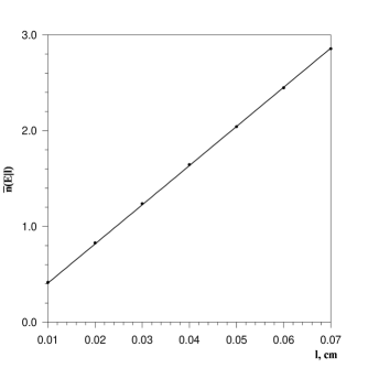
Fig. 1: Mean number of photons. solid line — Eq. (10), points — simulation.

Fig. 2: Energy distributions of emitted photons at l=0.01cm

For small $l$ when multiphoton effect can be neglected the energy distribution $P(E_{\gamma};E,l)$ can be expressed in terms of the differential cross section $\Sigma(E_{\gamma};E):$ $P(E_{\gamma};E,l)=l\Sigma(E_{\gamma};E).$ Fig.3 shows that the distribution $P(E_{\gamma};E,l)$ obtained by simulation agrees with that one calculated with using the formula (11).

Data on $\overline{Q}(E,l)$ are given in Fig.4 as well as the mean energy of emitted photons: $\overline{E_{\gamma}}=\frac{\overline{Q}}{\overline{n}}$. It is seen that $\overline{E_{\gamma}}$ slowly decreases with $l$ because of electron energy decreasing. The variance of energy loss $\sigma_{Q}^{2}(E,l)$ is shown in Fig.5. One can see that the analytical formulas (13), (14) for $\overline{Q}$ and $\sigma_{Q}^{2}$ agrees with the data of Monte Carlo simulation quite good.

The Monte Carlo code was used to calculate the probability density function $P(Q|E,l)$ describing the distribution of electrons over energy loss $Q$ and the ratio of $P(Q|E,l)$ to the energy spectra. The results are given in Fig.6 which displays the difference between radiation loss spectrum from finite thickness target and intensity spectrum of bremsstrahlung in the field of single nucleus. It is clear that multiphoton emission depresses the low energy part of the distribution and increases the high energy part. The effect rises with the target thickness increasing.

This work is supported by the Grant of the Ministry of General and Professional Education of the Russian Federation.

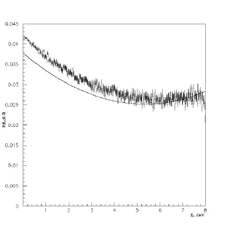
Fig. 3: Comparison of photons energy distribution corresponding to Eq. (11) (solid line) with simulation at $l=0.01cm$

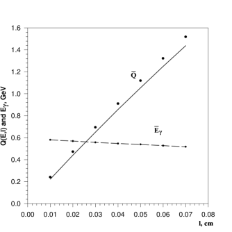
Fig. 4: Mean energy loss $\overline{Q}(E,l)$ and mean energy of emitted photons $\overline{E_{\gamma}}$. Solid line — Eq.  (13), points — simulation

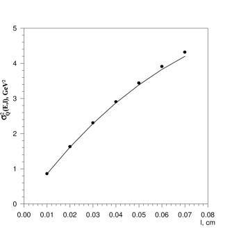
Fig. 5: Variance of energy loss. Solid line — Eq.  (14), points — simulation

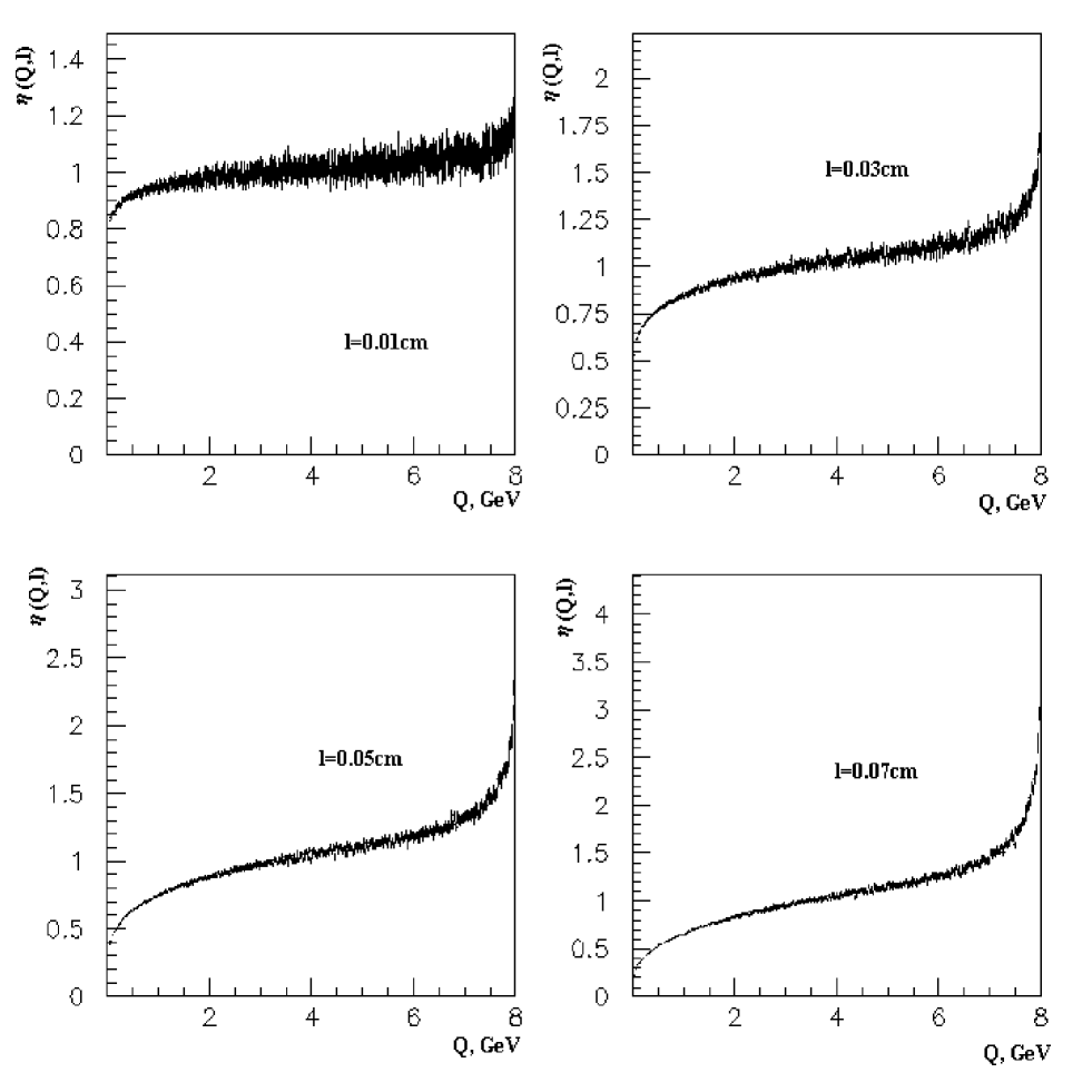
Fig. 6: The ratio $\eta(Q,l)=\frac{P(Q|E,l)}{P(E_{\gamma}=Q|E,l)}$

References

- [1] P.L.Anthony, R. Becker-Szendy, P.E.Bosted et al. Phys. Rev. Lett. 76 (1996) 3550.
- [2] V.N.Baier and V.M.Katkov Multi-Photon Effects in Energy Losses Spectra. Preprint BINP 98-24, 1998.
- [3] W. Feller. An Introduction to Probability Theory ant its Applications, v.II. John Willey&Sons, New York - London - Sydney - Toronto. 1971.
- [4] A.M.Kolchuzhkin, V.V.Uchaikin. Introduction into the Theory of Particles Penetration Through a Matter. (book in Russian) Moscow, Atomizdat, 1978.
- [5] M.L.Ter-Mikaelian. High Energy Electromagnetic Processes in Condensed Media, Whiley / Interscience, New York, 1972.
- [6] “GEANT, Detector Description and Simulation Tool”, CERN, Geneva, 1994.