Deeply virtual electroproduction of photons and mesons on the nucleon : leading order amplitudes and power corrections

Abstract

We estimate the leading order amplitudes for exclusive photon and meson electroproduction reactions at large $Q^{2}$ in the valence region in terms of skewed quark distributions. As experimental investigations can currently only be envisaged at moderate values of $Q^{2}$ , we estimate power corrections due to the intrinsic transverse momentum of the partons in the meson wavefunction and in the nucleon. To this aim the skewed parton distribution formalism is generalized so as to include the parton intrinsic transverse momentum dependence. Furthermore, for the meson electroproduction reactions, we calculate the soft overlap type contributions and compare with the leading order amplitudes. We give first estimates for these different power corrections in kinematics which are relevant for experiments in the near future.

PACS : 12.38.Bx, 13.60.Le, 13.60.Fz, 13.60.Hb

I Introduction

Much of the internal structure of the nucleon has been revealed during the last two decades through the inclusive scattering of high energy leptons on the nucleon in the Bjorken -or “Deep Inelastic Scattering” (DIS)- regime defined by $Q^{2},\nu\rightarrow\infty$ and $x_{B}=Q^{2}/2M\nu$ finite. Simple theoretical interpretations of the experimental results can be reached in the framework of QCD, when one sums over all the possible hadronic final states.
With the advent of the new generation of high-energy, high-luminosity lepton accelerators combined with large acceptance spectrometers, a wide variety of exclusive processes in the Bjorken regime are considered as experimentally accessible. In recent years, a unified theoretical description of such processes has emerged through the formalism introducing new generalized parton distributions, the so-called ‘Off-Forward Parton Distributions’ (OFPD’s), commonly also denoted as skewed parton distributions. It has been shown that these distributions, which parametrize the structure of the nucleon, allow to describe, in leading order perturbative QCD (PQCD), various exclusive processes in the near forward direction. The most promising ones are deeply Virtual Compton Scattering (DVCS) and longitudinal electroproduction of vector or pseudoscalar mesons (see Refs.[1]-[4] and references therein to other existing literature). Maybe most of the recent interest and activity in this field has been triggered by the observation of Ji [1], who showed that the second moment of these OFPD’s measures the contribution of the spin and orbital momentum of the quarks to the nucleon spin. Clearly this may shed a new light on the “spin-puzzle”.
In section II, we introduce the definitions and conventions of the skewed parton distributions. We also present the modelizations for these distributions that will be used in our cross section estimates.
In section III, the leading order PQCD amplitudes for DVCS and longitudinal electroproduction of mesons are presented in some detail. This is an extension of our previous works [5, 6].
In section IV, we investigate the power corrections to the leading order amplitudes when the virtuality of the photon is in the region $Q^{2}\approx 1-20$ GeV². The correction due to the intrinsic transverse momentum dependence is known to be important to get a successful description of the $\pi^{0}\gamma^{*}\gamma$ transition form factor, for which data exist in the range $Q^{2}\approx 1-10$ GeV². For the pion electromagnetic form factor in the transition region before asymptotia is reached, the power corrections due to both the transverse momentum dependence and the soft overlap mechanism are quantitatively important. We will therefore take these form factors as a guide to calculate the corrections due to the parton’s intrinsic transverse momentum dependence in the DVCS and hard meson electroproduction amplitudes. In addition, for the meson electroproduction amplitude, an estimate is given for the competing soft overlap mechanism, which - in contrast to the leading order perturbative mechanism - does not proceed through one-gluon exchange.
In section V, we give numerical estimates for different observables for DVCS and for the electroproduction of vector mesons $\rho^{(\pm,0)}$, $\omega$ and pseudoscalar mesons $\pi^{(\pm,0)}$, $\eta$. We give several examples of experimental opportunities to access the OFPD’s at the current high-energy lepton facilities : JLab ($E_{e}\geq$ 6 GeV) [7, 8], HERMES ($E_{e}$=27 GeV) and COMPASS ($E_{\mu}$=200 GeV).
Finally, we give our conclusions in section VI.

II Review of Skewed Parton Distributions

A Preliminary : bilocal operators and gauge invariance

In the following we often encounter bilocal products of quark fields $\psi$ at equal light-cone time of the form

$$\overline{\psi}(-y/2)\psi(y/2)\mid_{y^{+}=0}\;,$$ (1)

where $y^{+}$ is the light-cone time, with $y^{\pm}=(y^{0}\pm y^{3})/\sqrt{2}$. At leading twist one has the further restriction $\vec{y}_{\perp}=(y^{1},y^{2},0)=0$, that is the bilocal product needs only be evaluated along a light-cone segment of length $y^{-}$. For our purposes we need to consider the more general case where only $y^{+}$ is set to zero ( $y^{+}$ = 0 is understood in the remaining of this section).
The product of fields at different points is not invariant under a local color gauge transformation. To enforce gauge invariance, one replaces Eq. (1) by

$$\overline{\psi}(-y/2)L(-y/2\rightarrow y/2)\psi(y/2),$$ (2)

where the link operator $L$ is defined by

$$L(-y/2\rightarrow y/2)=P(e^{-i\int_{C}A.dl}).$$ (3)

In Eq. (3), the path ordered product is evaluated along a curve $C$ joining the points $-y/2$ and $y/2$ and $A$ is the matrix valued color gauge field. So in a general gauge, bilocal products of quark fields are not defined independently of the gauge field. To simplify the analysis it is therefore convenient to choose a curve $C$ and a gauge such that the link operator reduces to the identity.
Among the many possibilities we choose the curve shown on Fig. 1, where it is understood that $y^{+}=0$. We then split $L$ into 3 factors $L_{1},L_{2},L_{3}$ corresponding to the segments $C_{1},C_{2},C_{3}$ indicated on Fig. 1. We first go to the gauge where $A^{+}=0$ everywhere. This is always possible if one ignores the problems associated with the boundary conditions at infinity. Since we only deal with localised systems this is not a true restriction. In this gauge we have $L_{1}=L_{3}=1.$ While staying in the gauge $A^{+}=0$ we still have the freedom to make a gauge transformation which depends only on $(y^{1},y^{2}).$ This allows us to go to a gauge where $y^{1}A^{1}+y^{2}A^{2}=0$ in the plane $y^{-}=0.$ This is the 2-dimensional version of the radial, or Schwinger-Fock, gauge [9]. In this gauge we have $L_{2}=1$ which completes our argument, that is there exists a curve and a gauge such that the link operator is the identity operator. In the following it will always be understood that the bilocal quark field products (at $y^{+}=0$) are in this gauge , which is thus a convenient choice for model evaluations of the matrix elements of these operators.

B Definitions of skewed parton distributions

To set the framework of this work, we briefly review how the nonperturbative nucleon structure information enters the leading order PQCD amplitude for DVCS and hard meson electroproduction.
For DVCS, Ji [1] and Radyushkin [2] have shown that the leading order amplitude in the forward direction can be factorized in a hard scattering part (which is exactly calculable in PQCD) and a soft, nonperturbative nucleon structure part as is illustrated in Fig. 2. In these so-called “handbag” diagrams, the nucleon structure information can be parametrized, at leading order PQCD, in terms of four generalized structure functions, which conserve quark helicity. It was shown in Refs. [10, 11], that at leading twist, two more functions appear which involve a quark helicity flip. However, the authors of Ref. [12] have shown that in reactions which would involve these helicity flip distributions (such as exclusive electroproduction of transversely polarized vector mesons), this contribution vanishes due to angular momentum and chirality conservation in the hard scattering. This was argued [12] to hold at leading order in $1/Q$ and to all orders in perturbation theory. In this work, we will restrict ourselves to the four distributions which conserve quark helicity. Then, the matrix element of the bilocal quark operator, representing the lower blob in Figs. 2a and 2b, can be expressed at leading twist, in the notation of Ji, in terms of the OFPD’s $H,\tilde{H},E,\tilde{E}$ as :

$${{P^{+}}\over{2\pi}}\,\int dy^{-}e^{ixP^{+}y^{-}}\langle p^{{}^{\prime}}|\bar{\psi}_{\beta}(-{y\over 2})\psi_{\alpha}({y\over 2})|p\rangle{\Bigg{|}}_{y^{+}=\vec{y}_{\perp}=0}$$ (4)

$$={1\over 4}\left\{({\gamma^{-}})_{\alpha\beta}\left[{H^{q}(x,\xi,t)\;\bar{N}(p^{{}^{\prime}})\gamma^{+}N(p)\;+\;E^{q}(x,\xi,t)\;\bar{N}(p^{{}^{\prime}})i\sigma^{+\kappa}{{\Delta_{\kappa}}\over{2m_{N}}}N(p)}\right]\right.$$ (5)

$$\hskip 19.91684pt\left.+({\gamma_{5}\gamma^{-}})_{\alpha\beta}\left[{\tilde{H}^{q}(x,\xi,t)\;\bar{N}(p^{{}^{\prime}})\gamma^{+}\gamma_{5}N(p)\;+\;\tilde{E}^{q}(x,\xi,t)\;\bar{N}(p^{{}^{\prime}})\gamma_{5}{{\Delta^{+}}\over{2m_{N}}}N(p)}\right]\right\}\;,$$ (6)

where $\psi$ is the quark field, $N$ the nucleon spinor and $m_{N}$ the nucleon mass. In writing down Eq. (6) one uses a frame where the virtual photon momentum $q^{\mu}$ and the average nucleon momentum $P^{\mu}$ (see Fig. 2 for the kinematics) are collinear along the $z$-axis and in opposite direction. We denote the lightlike vectors along the positive and negative $z$-directions as $\tilde{p}^{\mu}=P^{+}/\sqrt{2}(1,0,0,1)$ and $n^{\mu}=1/P^{+}\cdot 1/\sqrt{2}(1,0,0,-1)$ respectively, and define light-cone components $a^{\pm}$ by $a^{\pm}\equiv(a^{0}\pm a^{3})/\sqrt{2}$. In this frame, the physical momenta have the following decomposition :

$$P^{\mu}={1\over 2}\left(p^{\mu}+p^{\prime\mu}\right)\;=\tilde{p}^{\mu}+{{\bar{m}^{2}}\over 2}\,n^{\mu}\;,$$ (7)

$$q^{\mu}=-\left(2\xi^{{}^{\prime}}\right)\,\tilde{p}^{\mu}+\left({{Q^{2}}\over{4\xi^{{}^{\prime}}}}\right)\,n^{\mu}\;,$$ (8)

$$\Delta^{\mu}\equiv p^{{}^{\prime}\mu}-p^{\mu}=-\left(2\xi\right)\,\tilde{p}^{\mu}+\left(\xi\,\bar{m}^{2}\right)\,n^{\mu}+\Delta^{\mu}_{\perp}\;,$$ (9)

$$q^{{}^{\prime}\mu}\equiv q^{\mu}-\Delta^{\mu}=-2\left(\xi^{{}^{\prime}}-\xi\right)\,\tilde{p}^{\mu}+\left({{Q^{2}}\over{4\xi^{{}^{\prime}}}}-\xi\,\bar{m}^{2}\right)\,n^{\mu}-\Delta^{\mu}_{\perp}\;,$$ (10)

where the variables $\bar{m}^{2}$, $\xi^{{}^{\prime}}$ and $\xi$ are given by

$$\bar{m}^{2}={m_{N}}^{2}-{{\Delta^{2}}\over 4}\;,$$ (11)

$$2\xi^{{}^{\prime}}={{P\cdot q}\over{\bar{m}^{2}}}\,\left[-1+\sqrt{1+{{Q^{2}\,\bar{m}^{2}}\over{(P\cdot q)^{2}}}}\right]\;\stackrel{{\scriptstyle Bj}}{{\longrightarrow}}\;\frac{x_{B}}{1-\frac{x_{B}}{2}}\;,$$ (12)

$$2\xi=2\xi^{{}^{\prime}}\,{{Q^{2}-\Delta^{2}}\over{Q^{2}+\bar{m}^{2}(2\xi^{{}^{\prime}})^{2}}}\;\stackrel{{\scriptstyle Bj}}{{\longrightarrow}}\;\frac{x_{B}}{1-\frac{x_{B}}{2}}\;.$$ (13)

In Eq. (6), the OFPD’s $H^{q},E^{q},\tilde{H}^{q},\tilde{E}^{q}$ are defined for one quark flavor ($q=u,d$ and $s$). The functions $H$ and $E$ are helicity averaged whereas $\tilde{H}$ and $\tilde{E}$ are helicity dependent functions. They depend upon three variables : $x$, $\xi$, $t$. The light-cone momentum fraction $x$ is defined by $k^{+}=xP^{+}$. The variable $\xi$ is defined by $\Delta^{+}=-2\xi\,P^{+}$, where $\Delta\equiv p^{{}^{\prime}}-p$ and $t=\Delta^{2}$. Note that $2\xi\rightarrow x_{B}/(1-x_{B}/2)$ in the Bjorken limit. The support in $x$ of the OFPD’s is $\left[-1,1\right]$ and a negative momentum fraction corresponds with the antiquark contribution.
To simplify the presentation, we will take $\xi^{{}^{\prime}}=\xi$ in the following. As shown in Eqs. (11-13), these two variables have the same value in the Bjorken limit. The kinematic variable $\xi$, which represents the longitudinal momentum fraction of the transfer $\Delta$, is bounded by

$$0<\xi<{{\sqrt{-\Delta^{2}}/2}\over{\bar{m}}}<1\;.$$ (14)

A glance at Figs. 2 a,b shows that the active quark with momentum $k-\Delta/2$ has longitudinal (+ component) momentum fraction $x+\xi$, whereas the one with momentum $k+\Delta/2$ has longitudinal momentum fraction $x-\xi$. As noted by Radyushkin [2], since negative momentum fractions correspond to antiquarks, one can identify two regions according to whether $|x|>\xi$ or $|x|<\xi$ .

• When $x>\xi$, both quark propagators represent quarks, whereas for $x<-\xi$ both represent antiquarks. In these regions, the OFPD’s are the generalizations of the usual parton distributions from DIS. Actually, in the forward direction, the OFPD’s $H$ and $\tilde{H}$ respectively reduce to the quark density distribution $q(x)$ and the quark helicity distribution $\Delta q(x)$ :

  $$H^{q}(x,0,0)\,=\,q(x)\;,\hskip 56.9055pt\tilde{H}^{q}(x,0,0)\,=\,\Delta q(x)\;,$$ (15)

  where $q$ and $\Delta q$ are defined by the Fourier integrals on the light cone [13] :

  $$q(x)\, = \,{{p^{+}}\over{4\pi}}\,\int dy^{-}e^{ixp^{+}y^{-}}\langle p|\bar{\psi}(0)\gamma.n\psi(y)|p\rangle{\Bigg{|}}_{y^{+}=\vec{y}_{\perp}=0}\;,$$ (16)

  $$\Delta q(x)\, = \,{{p^{+}}\over{4\pi}}\,\int dy^{-}e^{ixp^{+}y^{-}}\langle pS_{\|}|\bar{\psi}(0)\gamma.n\gamma_{5}\psi(y)|pS_{\|}\rangle{\Bigg{|}}_{y^{+}=\vec{y}_{\perp}=0}\;.$$ (17)

  In Eqs. (16, 17), $p$ represents the initial nucleon momentum in the DIS process and $S_{\|}$ is the longitudinal nucleon spin projection. From Eqs. (16, 17) the quark distributions for negative momentum fractions are related to the antiquark distributions as $q(-x)=-\,\bar{q}(x)$ and $\Delta q(-x)=+\,\Delta\bar{q}(x)$.

• In the region $-\xi<x<\xi$, one quark propagator represents a quark and the other one an antiquark. In this region, the OFPD’s behave like a meson distribution amplitude.

An alternative, but equivalent, parametrization of the matrix elements of the bilocal operators has been proposed by Radyushkin [2] by expressing the longitudinal momentum fractions with respect to the initial nucleon momentum $p$ instead of the average momentum $P$ of Fig. 2. In this notation, the active quark has momentum $k^{+}=Xp^{+}$ and $\Delta^{+}=-\zeta p^{+}$. The two variables $X$ and $\zeta$ are related to the previously introduced momentum fractions $x$ and $\xi$ by:

$$x\equiv{{X-\zeta/2}\over{1-\zeta/2}}\;,\hskip 14.22636pt\xi\equiv{{\zeta/2}\over{1-\zeta/2}}\;.$$ (18)

In terms of the variables $X$, $\zeta$ and $t$, so-called ‘non-forward parton distributions’ (NFPD’s) $f^{q}(X,\zeta,t)$ were introduced by Radyushkin [2]. They are equivalent to the OFPD’s and are related to them by

$$H^{q}(x,\xi,t)\, = \,{{1}\over{1+\xi}}\,\left\{\,f^{q}(X,\zeta,t)\,\right\}\;,\hskip 28.45274pt{\mathrm{f}or}\hskip 14.22636pt\xi\leq x\leq 1\;,$$ (19)

$$H^{q}(x,\xi,t)\, = \,{{1}\over{1+\xi}}\,\left\{\,f^{q}(X,\zeta,t)\;-\;f^{\bar{q}}(\zeta-X,\zeta,t)\,\right\}\;,\hskip 28.45274pt{\mathrm{f}or}\hskip 14.22636pt-\xi\leq x\leq\xi\;,$$ (20)

$$H^{q}(x,\xi,t)\, = \,{{1}\over{1+\xi}}\,\left\{\,-\,f^{\bar{q}}(\zeta-X,\zeta,t)\,\right\}\;,\hskip 28.45274pt{\mathrm{f}or}\hskip 14.22636pt-1\leq x\leq-\xi\;,$$ (21)

where $f^{q}$ are the quark and $f^{\bar{q}}$ the anti-quark NFPD’s respectively.
The “double” nature of the skewed parton distributions according to whether $0\leq x\leq\xi$ ($0\leq X\leq\zeta$) or $\xi\leq x\leq 1$ ($\zeta\leq X\leq 1$) was made more transparent by Radyushkin by expressing the quark momenta connected to the lower blob of Fig. 2 in a fraction $\tilde{x}$ of the initial nucleon momentum $p$ and a fraction $y$ of the momentum transfer $\Delta$ as shown in Fig. 3. The relation with the previously introduced momentum fraction $X$ is readily seen to be $X=\tilde{x}+\zeta y$. In terms of the variables $\tilde{x},y,t$, Radyushkin then introduced [2, 14] the so-called double distributions $F^{q}$, $K^{q}$ for quarks and $F^{\bar{q}}$, $K^{\bar{q}}$ for the anti-quarks, according to:

$$\langle p^{{}^{\prime}}|\bar{\psi}(0)\;\gamma^{+}\;\psi(z)|p\rangle{\Bigg{|}}_{z^{+}=\vec{z}_{\perp}=0}$$ (22)

$$=\bar{N}(p^{{}^{\prime}})\gamma^{+}N(p)\;\cdot\;\int_{0}^{1}d\tilde{x}\,\int_{0}^{1-\tilde{x}}dy\;\left\{e^{-i\left(\tilde{x}p^{+}\,-\,y\Delta^{+}\right)z^{-}}F^{q}(\tilde{x},y,t)\;-\;e^{i\left(\tilde{x}p^{+}\,+\,\bar{y}\Delta^{+}\right)z^{-}}F^{\bar{q}}(\tilde{x},y,t)\right\}$$ (23)

$$+\;\bar{N}(p^{{}^{\prime}})i\sigma^{+\kappa}{{\Delta_{\kappa}}\over{2m_{N}}}N(p)$$ (24)

$$\hskip 14.22636pt\times\int_{0}^{1}d\tilde{x}\,\int_{0}^{1-\tilde{x}}dy\;\left\{e^{-i\left(\tilde{x}p^{+}\,-\,y\Delta^{+}\right)z^{-}}K^{q}(\tilde{x},y,t)\;-\;e^{i\left(\tilde{x}p^{+}\,+\,\bar{y}\Delta^{+}\right)z^{-}}K^{\bar{q}}(\tilde{x},y,t)\right\}\;,$$ (25)

with both $\tilde{x}$ and $y$ positive and $\tilde{x}+y\leq 1$. The double distributions are related to the NFPD’s through integrals over $y$ [2, 14] :

$$f^{q}(X,\zeta,t)\,=\,\int_{0}^{\bar{X}/\bar{\zeta}}dy\;\;F^{q}(X-\zeta y,y,t)\;,\hskip 28.45274pt{\mathrm{f}or}\hskip 28.45274ptX\geq\zeta\;,$$ (26)

$$f^{q}(X,\zeta,t)\,=\,\int_{0}^{X/\zeta}dy\;\;F^{q}(X-\zeta y,y,t)\;,\hskip 28.45274pt{\mathrm{f}or}\hskip 28.45274ptX\leq\zeta\;,$$ (27)

with $\bar{X}\equiv 1-X$ and $\bar{\zeta}\equiv 1-\zeta$. Relations similar to Eq. (27) hold for the anti-quark distributions $f^{\bar{q}}$. Analogously to Eq. (25), one defines the helicity dependent double distributions $\tilde{F}$ and $\tilde{K}$ through the matrix element of a bilocal axial vector operator.
Besides coinciding with the quark distributions at vanishing momentum transfer, the skewed parton distributions have interesting links with other nucleon structure quantities. The first moments of the OFPD’s are related to the elastic form factors of the nucleon through model independent sum rules [1] . By integrating Eq. (6) over $x$, one gets the following relations for one quark flavor :

$$\int_{-1}^{+1}dx\;H^{q}(x,\xi,t)\,=\,F_{1}^{q}(t)\;,\hskip 14.22636pt\int_{-1}^{+1}dx\;E^{q}(x,\xi,t)\,=\,F_{2}^{q}(t)\;,$$ (28)

$$\int_{-1}^{+1}dx\;\tilde{H}^{q}(x,\xi,t)\,=\,g_{A}^{q}(t)\;,\hskip 14.22636pt\int_{-1}^{+1}dx\;\tilde{E}^{q}(x,\xi,t)\,=\,h_{A}^{q}(t)\;.$$ (29)

The elastic form factors for one quark flavor on the RHS of Eqs. (28, 29) have to be related to the physical ones. Restricting to the $u,d$ and $s$ quark flavors, the Dirac form factors are expressed as

$$F_{1}^{u/p}\,=\,2F_{1}^{p}+F_{1}^{n}+F_{1}^{s}\;,\hskip 14.22636ptF_{1}^{d/p}\,=\,2F_{1}^{n}+F_{1}^{p}+F_{1}^{s}\;,$$ (30)

where $F_{1}^{p}$ and $F_{1}^{n}$ are the proton and neutron electromagnetic form factors respectively. The strange form factor is given by $F_{1}^{s/p}\equiv F_{1}^{s}$, but since it is small and not so well known we set it to zero in the following numerical evaluations. Relations similar to Eq. (30) hold for the Pauli form factors $F_{2}^{q}$. For the axial vector form factors one uses the isospin decomposition :

$$g_{A}^{u/p}\,=\,{1\over 2}g_{A}+{1\over 2}g_{A}^{0}\;,\hskip 14.22636ptg_{A}^{d/p}\,=\,-{1\over 2}g_{A}+{1\over 2}g_{A}^{0}\;.$$ (31)

The isovector axial form factor $g_{A}$ is known from experiment, with $g_{A}(0)\approx 1.267$ [15]. For the unknown isoscalar axial form factor $g_{A}^{0}$, we use the quark model relation : $g_{A}^{0}(t)=3/5\,g_{A}(t)$. For the pseudoscalar form factor $h_{A}^{q}$, we have relations similar to Eq. (31).
The second moment of the OFPD’s is relevant for the nucleon spin structure. It was shown in Ref. [1] that there exists a (color) gauge-invariant decomposition of the nucleon spin :

$${1\over 2}\,=\,J_{q}\,+\,J_{g}\;,$$ (32)

where $J_{q}$ and $J_{g}$ are respectively the total quark and gluon angular momentum. The second moment of the unpolarized OFPD’s at $t=0$ gives

$$J_{q}\,=\,{1\over 2}\,\int_{-1}^{+1}dx\,x\,\left[H^{q}(x,\xi,t=0)+E^{q}(x,\xi,t=0)\right]\;,$$ (33)

and this relation is independent of $\xi$. The quark angular momentum $J_{q}$ decomposes as

$$J_{q}={1\over 2}\Delta\Sigma+L_{q}\;,$$ (34)

where $\Delta\Sigma/2$ and $L_{q}$ are respectively the quark spin and orbital angular momentum. As $\Delta\Sigma$ is measured through polarized DIS experiments, a measurement of the sum rule of Eq. (33) in terms of the OFPD’s, provides a model independent way to determine the quark orbital contribution to the nucleon spin and thus from Eq. (32) the gluon contribution.

C Modelization of the skewed parton distributions

Ultimately one wants to extract the skewed parton distributions from the data but, in order to evaluate electroproduction observables, we need a first guess for them. We shall restrict our considerations to the near forward direction because this kinematical domain is the closest to inclusive DIS, which we want to use as a guide. Since $E$ and $\tilde{E}$ are always multiplied by the momentum transfer, this means that the amplitudes are dominated by $H$ and $\tilde{H}$ which we discuss first.

1 $\xi$-independent ansatz for $H$ and $\tilde{H}$

The simplest ansatz, already used in our previous works [5, 6], is to write $H$ and $\tilde{H}$ as a product of a form factor and a quark distribution function, neglecting any $\xi$ dependence, which yields :

$$H^{u/p}(x,\xi,t)=u(x)\,{F_{1}^{u/p}(t)}/2\;,\hskip 14.22636ptH^{d/p}(x,\xi,t)=d(x)\,{F_{1}^{d/p}(t)}\;,\hskip 14.22636ptH^{s/p}(x,\xi,t)=0\;,$$ (35)

where $u(x),d(x)$ and $s(x)$ are the unpolarized quark distributions. Obviously the ansatz of Eq. (35) satisfies both Eq. (15) and the sum rule of Eq. (28), if one uses the valence quark distributions normalized as:

$${1\over 2}\int_{0}^{+1}dx\;u_{V}(x)=\int_{0}^{+1}dx\;d_{V}(x)=1\;.$$ (36)

For all the calculations presented in this paper, we shall use the parametrization MRST98 [17] for the quark distributions.

To model $\tilde{H}^{q}$, we need the corresponding polarized quark distributions. For this we follow the recent work of Ref.[16], where a next to leading order QCD analysis of inclusive polarized deep-inelastic lepton-nucleon scattering was performed and which yields an excellent fit of the world data. In this analysis, the input polarized densities (at a scale $Q_{0}^{2}$ = 1 GeV²) are given by :

$$\Delta u_{V}(x,Q_{0}^{2})=\eta_{u}\,A_{u}\;x^{0.250}\;u_{V}(x,Q_{0}^{2})\;,$$ (37)

$$\Delta d_{V}(x,Q_{0}^{2})=\eta_{d}\,A_{d}\;x^{0.231}\;d_{V}(x,Q_{0}^{2})\;,$$ (38)

$$\Delta\bar{q}(x,Q_{0}^{2})=\eta_{\bar{q}}\,A_{S}\;x^{0.576}\;S(x,Q_{0}^{2})\;,$$ (39)

where we assume a SU(3) symmetric sea, i.e. $\Delta\bar{q}\equiv\Delta\bar{u}$ = $\Delta\bar{d}$ = $\Delta\bar{s}$ and $S$ represents the total sea. On the rhs of Eqs. (39), the normalization factors $A_{u},A_{d},A_{S}$ are determined so that the first moments of the polarized densities are given by $\eta_{u},\eta_{d},\eta_{\bar{q}}$ respectively. For the valence quark densities, $\eta_{u}$ and $\eta_{d}$ were fixed in Ref.[16] by the octet hyperon $\beta$ decay constants which yield :

$$\eta_{u}\;=\;\int_{0}^{+1}dx\;\Delta u_{V}(x)\;\approx 0.918\;,\hskip 28.45274pt\eta_{d}\;=\;\int_{0}^{+1}dx\;\Delta d_{V}(x)\;\approx-0.339\;.$$ (40)

The first moment of the polarized sea quark density was determined by the fit of Ref.[16] which gives $\eta_{\bar{q}}\approx-0.054$.
Our ansatz for $\tilde{H}^{q}$ is to multiply the polarized quark distributions of Eq. (39) by the axial form factor, neglecting any $\xi$-dependence and sea contribution, which yields

$$\tilde{H}^{u/p}(x,\xi,t)=\Delta u_{V}(x)\,{g_{A}^{u/p}(t)}/{g_{A}^{u/p}(0)}\;,\hskip 14.22636pt\tilde{H}^{d/p}(x,\xi,t)=\Delta d_{V}(x)\,{g_{A}^{d/p}(t)}/{g_{A}^{d/p}(0)}\;.$$ (41)

One can check that Eq. (15) is verified by construction and that, using the (31) and the quark model relation to evaluate the axial form factors $g_{A}^{u/p}$ and $g_{A}^{d/p}$, the sum rule of Eq. (29) is satisfied within 10 %.

2 $\xi$-dependent ansatz for $H$ and $\tilde{H}$

To generate the dependence on $\xi$, we start from the double distributions introduced in Eq. (25). As shown in Fig. 3, the momentum flow in the double distributions is decomposed in a part along the initial nucleon momentum $p$ and a part along the momentum transfer $\Delta$ . Therefore, a reasonable guess for the helicity independent double distribution $F(\tilde{x},y,t)$ was proposed in Ref.[14], as a product of a quark distribution function $q(\tilde{x})$, describing the momentum flow along $p$, and an asymptotic “meson-like” distribution amplitude $\sim y(1-\tilde{x}-y)$, describing the momentum flow along $\Delta$. Properly normalized, this yields :

$$F^{q}(\tilde{x},y,t)\;=\;F_{1}^{q}(t)/F_{1}^{q}(0)\;q(\tilde{x})\;6\,{{y(1-\tilde{x}-y)}\over{(1-\tilde{x})^{3}}}\;,$$ (42)

where similarly to Eq. (35), the $t$-dependent part is given by the form factor $F_{1}$. Similarly for the helicity dependent double distribution, this ansatz yields :

$$\tilde{F}^{q}(\tilde{x},y,t)\;=\;g_{A}^{q}(t)/g_{A}^{q}(0)\;\Delta q(\tilde{x})\;6\,{{y(1-\tilde{x}-y)}\over{(1-\tilde{x})^{3}}}\;,$$ (43)

Starting from Eq.(42), the OFPD $H^{q}$ is then constructed by using Eqs. (21) and (27). Analogously, the OFPD $\tilde{H}^{q}$ is constructed starting from Eq. (43).

As an example, we show on Fig. 5 the dependence on $\xi$ predicted by this model for the valence $d$-quark and total $d$-quark skewed distributions.

3 The skewed distributions $E$ and $\tilde{E}$

The modelization of $E$ and $\tilde{E}$, which correspond to helicity flip amplitudes, is more difficult as we don’t have the DIS constraint for the $x$-dependence in the forward limit. However, as already pointed out, $E$ and $\tilde{E}$ are multiplied by a momentum transfer and therefore their contribution is suppressed at small $t$. Nevertheless it was argued by the authors of Ref.[18] that the pion exchange, which contributes to the region $-\xi\leq x\leq\xi$ of $\tilde{E}$, may be non negligible at small $t$ due to the proximity of the pion pole at $t=m_{\pi}^{2}$. We follow therefore the suggestion of Refs.[18, 19] and evaluate $\tilde{E}$ assuming it is entirely due to the pion pole. (By contrast we continue to neglect the contributions due to $E$ since there is no dangerous pole in this case). According to this hypothesis, since the pion exchange is isovector, we must have

$$\tilde{E}^{u/p}=-\tilde{E}^{d/p}={1\over 2}\;\tilde{E}_{\pi-pole}\;.$$ (44)

The $t$ -dependence of $\tilde{E}_{\pi-pole}(x,\xi,t)$ is fixed by the sum rule (29) pseudoscalar form factor $h_{A}(t)$ :

$$\int_{-1}^{+1}dx\;\tilde{E}^{(3)}(x,\xi,t)\,=\,h_{A}(t)\longrightarrow{{g_{A}\;\left(2M_{N}\right)^{2}}\over{-t+m_{\pi}^{2}}}\;,$$ (45)

where $\tilde{E}^{(3)}\equiv\tilde{E}^{u/p}-\tilde{E}^{d/p}$ denotes the isovector OFPD and where we have approximated the pseudoscalar form factor by its pion pole dominance expression.

In the region $-\xi\leq x\leq\xi$, the quark and antiquark couple to the pion field of the nucleon. Therefore, this coupling should be proportional to the pion distribution amplitude. For the later we take the asymptotic form, which is well supported now by experiment (see discussion in section IV A). Expressing the quark’s longitudinal momentum fraction $z$ in the pion in the symmetric range $-1\leq z\leq 1$, the asymptotic distribution amplitude $\Phi_{as}$ is given by $\Phi_{as}(z)=3/4$ $(1-z^{2})$, and is normalized as $\int_{-1}^{+1}dz\;\Phi_{as}(z)=1$. The light-cone momentum fractions of the quark and antiquark in the pion which couples to the lower blobs in Figs. 2, 4, are respectively given by $(1+x/\xi)/2$ and $(1-x/\xi)/2$. Therefore, $\tilde{E}_{\pi-pole}$ is finally modelled as

$$\tilde{E}_{\pi-pole}\;=\;\Theta\left(-\xi\leq x\leq\xi\right)\;h_{A}(t)\;{1\over\xi}\;\Phi_{as}\left({x\over\xi}\right)\;,$$ (46)

which satisfies the sum rule of Eq. (45).

As there is no dangerous pole in the case of $E$, it seems safe to neglect its contribution to the amplitude at small $t$, which of course does not mean that $E$ itself is small. In this respect it is amusing to note that, if one adopts for $E$ an ansatz similar to the one for $H$, Eq. (35), that is

$$E^{u/p}(x,\xi,t)=u(x)\,{F_{2}^{u/p}(t)}/2\;,\hskip 14.22636ptE^{d/p}(x,\xi,t)=d(x)\,{F_{2}^{d/p}(t)}\;,\hskip 14.22636ptE^{s/p}(x,\xi,t)=0\;,$$ (47)

and if one uses this ansatz to evaluate the total spin carried by the quarks through the sum rule of Eq. (33), one get the results shown in Table I. We can see that, even though there is little theoretical basis for the ansatz of Eq. (47), we get the reasonable result that 43% of the nucleon spin in carried by the quarks. This is consistent with a recent QCD sum rule estimate [23] (at a low scale) where the gluons were found to contribution to half of the nucleon spin. Note that only the information from the unpolarized parton distributions has been used to evaluate the quark contribution to the spin of the nucleon.

By using the decomposition of the total quark spin $J_{q}$ as in Eq. (34) and by using the most recent values measured at SMC [24] for the quark helicity distributions $\Delta u$, $\Delta d$ and $\Delta s$, one can extract the quark orbital angular momentum contribution to the nucleon spin. Using the factorized, $\xi$-independent ansatz, the orbital contribution is estimated in Table I to yield about 15% of the nucleon spin.

4 Other models of the skewed distributions

Some model calculations of the skewed distributions exist. A bag model evaluation of the skewed distributions [20] found (at a low scale) that they depend weakly on $\xi$. However, a calculation in the chiral quark soliton model [21] found (also at a low scale) a strong dependence on $\xi$ and exhibits in particular fast “crossovers” at $|x|=\xi$. The chiral quark soliton model is based on the large-$N_{c}$ picture of the nucleon as a heavy semiclassical system whose $N_{c}$ valence quarks are bound by a self-consistent pion field. The crossovers in this model can be interpreted as being due to meson-exchange type contributions in the region $-\xi\leq x\leq\xi$, which are not present in the bag model calculation and which are also not contained in the phenomenological ansatz of Eqs. (42, 43) for the double distributions (see Ref.[22] for a detailed discussion of these meson-exchange type contributions to the skewed quark distributions). It was noticed in Ref.[21] that this crossover behavior at $|x|=\xi$ could lead to an enhancement of observables, which will be interesting to quantify.

As a last remark, as we are mainly interested in this paper in giving estimates for electroproduction reactions in the valence region at only moderately large values of $Q^{2}$ ($1\sim 20$ GeV²), which is where experiments of exclusive electroproduction reactions can be performed currently or in the near future, we neglect here the scale dependence of the skewed distributions. At very high values of $Q^{2}$, the scale dependence should be considered. This scale dependence is described by generalized evolution equations that are under intensive investigation in the literature.

III Leading order amplitudes for DVCS and hard electroproduction of mesons

A DVCS

Factorization proofs for DVCS have been given by several authors [25, 26]. They give the theoretical underpinning which allows to express the leading order DVCS amplitude in terms of OFPD’s. Using the parametrization of Eq. (6), the leading order DVCS tensor $H^{\mu\nu}_{L.O.\,DVCS}$ follows from the two handbag diagrams of Fig. 2 as

$$H^{\mu\nu}_{L.O.\,DVCS}$$ (48)

$$= {1\over 2}\,\left[\tilde{p}^{\mu}n^{\nu}+\tilde{p}^{\nu}n^{\mu}-g^{\mu\nu}\right]\;\int_{-1}^{+1}dx\left[{1\over{x-\xi+i\epsilon}}+{1\over{x+\xi-i\epsilon}}\right]$$ (50)

$$\hskip 14.22636pt\times\left[H^{p}_{DVCS}(x,\xi,t)\;\bar{N}(p^{{}^{\prime}})\gamma.nN(p)+\;E^{p}_{DVCS}(x,\xi,t)\;\bar{N}(p^{{}^{\prime}})i\sigma^{\kappa\lambda}{{n_{\kappa}\Delta_{\lambda}}\over{2m_{N}}}N(p)\right]$$

$$+ \;{1\over 2}\,\left[-i\varepsilon^{\mu\nu\kappa\lambda}\tilde{p}_{\kappa}n_{\lambda}\right]\;\int_{-1}^{+1}dx\left[{1\over{x-\xi+i\epsilon}}-{1\over{x+\xi-i\epsilon}}\right]$$ (52)

$$\hskip 14.22636pt\times\left[\tilde{H}^{p}_{DVCS}(x,\xi,t)\bar{N}(p^{{}^{\prime}})\gamma.n\gamma_{5}N(p)+\tilde{E}^{p}_{DVCS}(x,\xi,t)\bar{N}(p^{{}^{\prime}})\gamma_{5}{{\Delta\cdot n}\over{2m_{N}}}N(p)\right]\;,$$

with $\varepsilon_{0123}=+1$. We refer to Ref.[6] for the formalism to calculate DVCS observables starting from the DVCS tensor of Eq. (52).
In the DVCS on the proton, the OFPD’s enter in the combination

$$H^{p}_{DVCS}(x,\xi,t)\,=\,{4\over 9}H^{u/p}\,+\,{1\over 9}H^{d/p}\,+\,{1\over 9}H^{s/p}\;,$$ (53)

and similarly for $\tilde{H}$, $E$ and $\tilde{E}$.
For the $\pi^{0}$ pole contribution to the DVCS amplitude, which contributes to the function $\tilde{E}^{p}_{DVCS}$, the convolution integral in Eq. (52) can be worked out analytically. By using Eqs. (44, 46) one obtains :

$$\int_{-1}^{+1}dx\left[{1\over{x-\xi+i\epsilon}}-{1\over{x+\xi-i\epsilon}}\right]\;\tilde{E}^{p}_{DVCS}(x,\xi,t)\;=\;-\,{1\over{2\xi}}\;h_{A}(t)\;.$$ (54)

The leading order DVCS amplitude of Eq. (52), is exactly gauge invariant with respect to the virtual photon, i.e. $q_{\nu}\,H^{\mu\nu}_{L.O.\,DVCS}=0$. However, electromagnetic gauge invariance is violated by the real photon except in the forward direction. In fact $q^{{}^{\prime}}_{\mu}\,H^{\mu\nu}_{L.O.DVCS}\sim\Delta_{\perp}$. This violation of gauge invariance is a higher twist effect of order $1/Q^{2}$ compared to the leading order term $H^{\mu\nu}_{L.O.\,DVCS}$. So in the limit $Q^{2}\rightarrow\infty$ it is innocuous but for actual experiments it matters. Actually for any cross section estimate one needs to choose a gauge and this explicit gauge dependence for nonzero angles is unpleasant. In the absence of a dynamical gauge invariant higher twist calculation of the DVCS amplitude, we propose to restore gauge invariance in a heuristic way based on physical considerations. We propose to introduce the gauge invariant tensor $H^{\mu\nu}_{DVCS}$ :

$$H^{\mu\nu}_{DVCS}\,=\,H^{\mu\nu}_{L.O.\,DVCS}\,-\,{{a^{\mu}}\over{\left(a\cdot q^{{}^{\prime}}\right)}}\;\left(q^{{}^{\prime}}_{\lambda}\,H^{\lambda\nu}_{L.O.\,DVCS}\right)\;,$$ (55)

where $a^{\mu}$ is a four-vector specified below. Obviously $H^{\mu\nu}_{DVCS}$ respects gauge invariance for both the virtual and the real photon :

$$q_{\nu}\,H^{\mu\nu}_{DVCS}=0\;,\hskip 28.45274ptq^{{}^{\prime}}_{\mu}\,H^{\mu\nu}_{DVCS}=0\;.$$ (56)

Furthermore, as

$$q^{{}^{\prime}}_{\lambda}\,H^{\lambda\nu}_{L.O.\,DVCS}=-\left(\Delta_{\perp}\right)_{\lambda}H^{\lambda\nu}_{L.O.\,DVCS}\;,$$ (57)

the gauge restoring term gives zero in the forward direction ($\Delta_{\perp}=0$) which is natural. We choose $a^{\mu}=\tilde{p}^{\mu}$ because $\tilde{p}\cdot q^{{}^{\prime}}$ is of order $Q^{2}$, which gives automatically a gauge restoring term of order $O\left(1/Q^{2}\right)$. This choice for $a^{\mu}$ is furthermore motivated by the fact that in the derivation of the leading order amplitude of Eq. (52), only the $\tilde{p}^{\mu}$ components at the electromagnetic vertices are retained [1]. The above arguments lead to the following DVCS amplitude:

$$H^{\mu\nu}_{DVCS}\,=\,H^{\mu\nu}_{L.O.\,DVCS}\,+\,{{\tilde{p}^{\mu}}\over{\left(\tilde{p}\cdot q^{{}^{\prime}}\right)}}\;\left(\Delta_{\perp}\right)_{\lambda}\,H^{\lambda\nu}_{L.O.\,DVCS}\;,$$ (58)

which is now gauge invariant with respect to both the virtual and real photons. We will illustrate the influence of this gauge invariance prescription, by comparing DVCS observables calculated with Eq. (58) and with the leading order formula of Eq. (52).

B Hard electroproduction of mesons

The OFPD’s reflect the structure of the nucleon independently of the reaction which probes the nucleon. In this sense, they are universal quantities and can also be accessed, in different flavor combinations, through the hard exclusive electroproduction of mesons - $\pi^{0,\pm},\eta,...,\rho^{0,\pm},\omega,\phi,...$ - (see Fig. 4) for which a QCD factorization proof was given in Refs. [3, 4]. According to Ref. [4], the factorization applies when the virtual photon is longitudinally polarized because in this case, the end-point contributions in the meson wave function are power suppressed. Furthermore, it was shown that the cross section for a transversely polarized photon is suppressed by 1/$Q^{2}$ compared to a longitudinally polarized photon.
Collins et al. [4] also showed that leading order PQCD predicts that the longitudinally polarized vector meson channels ($\rho^{0,\pm}_{L}$, $\omega_{L}$, $\phi_{L}$) are sensitive only to the unpolarized OFPD’s ($H$ and $E$) whereas the pseudo-scalar channels ($\pi^{0,\pm},\eta,...$) are sensitive only to the polarized OFPD’s ($\tilde{H}$ and $\tilde{E}$). It was shown in Ref.[12] that the leading twist contribution to exclusive electroproduction of transversely polarized vectors mesons vanishes at all orders in perturbation theory. In comparison to meson electroproduction reactions, we recall that DVCS depends at the same time on both the unpolarized ($H$ and $E$) and polarized ($\tilde{H}$ and $\tilde{E}$) OFPD’s.
According to the above discussion, we give predictions only for the meson electroproduction cross section by a longitudinal virtual photon. The longitudinal $\gamma^{*}_{L}+p\rightarrow M+p$ two-body cross section $d\sigma_{L}/dt$ is

$${{d\sigma_{L}}\over{dt}}={1\over{16\pi\left(s-m_{N}^{2}\right)\Lambda(s,-Q^{2},m_{N}^{2})}}\;{1\over 2}\sum_{h_{N}}\sum_{h^{{}^{\prime}}_{N}}|{\mathcal{M}}^{L}(\lambda_{M}=0,h^{{}^{\prime}}_{N};h_{N})|^{2}\;,$$ (59)

where $h_{N}$, $h^{{}^{\prime}}_{N}$ are the initial and final nucleon helicities and where the standard kinematic function $\Lambda(x,y,z)$ is defined by

$$\Lambda(x,y,z)=\sqrt{x^{2}+y^{2}+z^{2}-2xy-2xz-2yz}\;.$$ (60)

which gives $\Lambda(s,-Q^{2},m_{N}^{2})=2m_{N}|\vec{q}_{L}|$, where $|\vec{q}_{L}|$ is the virtual photon momentum in the lab system. As the way to extract $d\sigma_{L}/dt$ from the fivefold electroproduction cross section is a matter of convention, all results for $d\sigma_{L}/dt$ in this paper are given with the choice of the flux factor of Eq. (59).
In Eq. (59), ${\mathcal{M}}^{L}$ is the amplitude for the production of a meson with $\lambda_{M}=0$ by a longitudinal photon. In the valence region, the leading order amplitude is given by the hard scattering diagrams of Fig. 6 ($T_{H}$ part in Fig. 4). The amplitudes ${\mathcal{M}}^{L}$ for $\rho^{0}_{L}$ and $\pi^{0}$ electroproduction were calculated in Refs. [5] (see also Ref. [27]) for which the following gauge invariant expressions were found :

$${\mathcal{M}}^{L}_{\rho^{0}_{L}}=\;-ie\,{4\over 9}\,{1\over{Q}}\;\left[\,\int_{0}^{1}dz{{\Phi_{\rho}(z)}\over z}\right]\,{1\over 2}\,\int_{-1}^{+1}dx\left[{1\over{x-\xi+i\epsilon}}+{1\over{x+\xi-i\epsilon}}\right]$$ (61)

$$\hskip 56.9055pt\times(4\pi\alpha_{s})\;\left\{H^{p}_{\rho^{0}_{L}}(x,\xi,t)\bar{N}(p^{{}^{\prime}})\gamma.nN(p)+E^{p}_{\rho^{0}_{L}}(x,\xi,t)\bar{N}(p^{{}^{\prime}})i\sigma^{\kappa\lambda}{{n_{\kappa}\Delta_{\lambda}}\over{2m_{N}}}N(p)\right\},$$ (62)

$${\mathcal{M}}^{L}_{\pi^{0}}=\;-ie\,{4\over 9}\,{1\over{Q}}\;\left[\int_{0}^{1}dz{{\Phi_{\pi}(z)}\over z}\right]\,{1\over 2}\,\int_{-1}^{+1}dx\left[{1\over{x-\xi+i\epsilon}}+{1\over{x+\xi-i\epsilon}}\right]$$ (63)

$$\hskip 56.9055pt\times(4\pi\alpha_{s})\;\left\{\tilde{H}^{p}_{\pi^{0}}(x,\xi,t)\bar{N}(p^{{}^{\prime}})\gamma.n\gamma_{5}N(p)+\tilde{E}^{p}_{\pi^{0}}(x,\xi,t)\bar{N}(p^{{}^{\prime}})\gamma_{5}{{\Delta\cdot n}\over{2m_{N}}}N(p)\right\},$$ (64)

where $\Phi_{\rho}(z)$ and $\Phi_{\pi}(z)$ are the $\rho$ and $\pi$ distribution amplitudes (DA) respectively. The factor 4/9 is a color factor corresponding with one-gluon exchange. From Eqs. (62, 64), one sees that the leading order longitudinal amplitude for meson electroproduction behaves as $1/Q$. As the phase space factor in the cross section Eq. (59) behaves as $1/Q^{4}$ at fixed $x_{B}$ and fixed $t$, this leads to a $1/Q^{6}$ behavior of $d\sigma_{L}/dt$ at large $Q^{2}$ and at fixed $x_{B}$ and fixed $t$.
According to the considered reaction, the proton OFPD’s enter in different combinations due to the charges and isospin factors. For the electroproduction of $\rho^{0}$, which corresponds to the quark state (with spin $S=1$)

$$|\rho^{0}\rangle\;=\;{1\over\sqrt{2}}\left\{|u\bar{u}\rangle\;-\;|d\bar{d}\rangle\right\}\;,$$ (65)

the corresponding skewed distribution is given by:

$$H^{p}_{\rho^{0}_{L}}(x,\xi,t)\;=\;{1\over{\sqrt{2}}}\left\{{2\over 3}H^{u/p}\,+\,{1\over 3}H^{d/p}\right\}\;.$$ (66)

For the longitudinal electroproduction of the $\omega_{L}$ and $\phi_{L}$ vector mesons, the amplitudes have an expression analogous to Eq. (62) in terms of $H^{p}_{\omega_{L}}$ and $H^{p}_{\phi_{L}}$. By considering the $\omega$ and $\phi$ mesons as pure quark states (with $S=1$)

$$|\omega\rangle\;=\;{1\over\sqrt{2}}\left\{|u\bar{u}\rangle\;+\;|d\bar{d}\rangle\right\}\;,\hskip 28.45274pt|\phi\rangle\;=\;|s\bar{s}\rangle\;,$$ (67)

one then obtains for the corresponding OFPD’s :

$$H^{p}_{\omega_{L}}(x,\xi,t)\; = \;{1\over{\sqrt{2}}}\left\{{2\over 3}H^{u/p}\,-\,{1\over 3}H^{d/p}\right\}\;,$$ (68)

$$H^{p}_{\phi_{L}}(x,\xi,t)\; = \;-\;{1\over 3}H^{s/p}\;.$$ (69)

Besides the longitudinal electroproduction amplitude Eq. (64) for $\pi^{0}$, one again has analogous expressions for other neutral pseudoscalar mesons such as the $\eta$. Starting from the quark states (with spin S = 0) for pseudoscalar mesons and neglecting any mixing for the $\eta$ :

$$|\pi^{0}\rangle\; = \;{1\over\sqrt{2}}\left\{|u\bar{u}\rangle\;-\;|d\bar{d}\rangle\right\}\;,$$ (70)

$$|\eta\rangle\; = \;{1\over\sqrt{6}}\left\{|u\bar{u}\rangle\;+\;|d\bar{d}\rangle\;-\;2\;|s\bar{s}\rangle\right\}\;,$$ (71)

one obtains for the polarized OFPD’s :

$$\tilde{H}^{p}_{\pi^{0}}(x,\xi,t)\; = \;{1\over{\sqrt{2}}}\left\{{2\over 3}\tilde{H}^{u/p}\,+\,{1\over 3}\tilde{H}^{d/p}\right\}\;,$$ (72)

$$\tilde{H}^{p}_{\eta}(x,\xi,t)\; = \;{1\over{\sqrt{6}}}\left\{{2\over 3}\tilde{H}^{u/p}\,-\,{1\over 3}\tilde{H}^{d/p}\,+\,{2\over 3}\tilde{H}^{s/p}\right\}\;.$$ (73)

For the charged meson channels $\rho^{\pm}$ and $\pi^{\pm}$, we obtain from $|\rho^{+}>=-|u\bar{d}>$ and $|\rho^{-}>=|d\bar{u}>$ for the corresponding longitudinal electroproduction amplitudes (which have been given previously for the $\rho^{\pm}$ in Ref.[28] and for the $\pi^{\pm}$ in Refs.[29, 19]) :

$${\mathcal{M}}^{L}_{\rho^{\pm}}=\;-ie\,{4\over 9}\,{1\over{Q}}\;\left[\,\int_{0}^{1}dz{{\Phi_{\rho}(z)}\over z}\right]\,$$ (74)

$$\hskip 42.67912pt\times{1\over 2}\,\int_{-1}^{+1}dx\left[\left\{\begin{array}[]{c}-2/3\\ -1/3\end{array}\right\}{1\over{x-\xi+i\epsilon}}+\left\{\begin{array}[]{c}1/3\\ 2/3\end{array}\right\}{1\over{x+\xi-i\epsilon}}\right]$$ (79)

$$\hskip 42.67912pt\times(4\pi\alpha_{s})\;\left\{H^{(3)}(x,\xi,t)\bar{N}(p^{{}^{\prime}})\gamma.nN(p)+E^{(3)}(x,\xi,t)\bar{N}(p^{{}^{\prime}})i\sigma^{\kappa\lambda}{{n_{\kappa}\Delta_{\lambda}}\over{2m_{N}}}N(p)\right\}\;,$$ (80)

$${\mathcal{M}}^{L}_{\pi^{\pm}}=\;-ie\,{4\over 9}\,{1\over{Q}}\;\left[\int_{0}^{1}dz{{\Phi_{\pi}(z)}\over z}\right]\,$$ (81)

$$\hskip 42.67912pt\times{1\over 2}\,\int_{-1}^{+1}dx\left[\left\{\begin{array}[]{c}-2/3\\ -1/3\end{array}\right\}{1\over{x-\xi+i\epsilon}}+\left\{\begin{array}[]{c}1/3\\ 2/3\end{array}\right\}{1\over{x+\xi-i\epsilon}}\right]$$ (86)

$$\hskip 42.67912pt\times(4\pi\alpha_{s})\;\left\{\tilde{H}^{(3)}(x,\xi,t)\bar{N}(p^{{}^{\prime}})\gamma.n\gamma_{5}N(p)+\tilde{E}^{(3)}(x,\xi,t)\bar{N}(p^{{}^{\prime}})\gamma_{5}{{\Delta\cdot n}\over{2m_{N}}}N(p)\right\}\;,$$ (87)

where the $u$- and $d$-quark charges appear in front of the direct and crossed terms and where the following isovector forms for the corresponding OFPD’s enter :

$$H^{(3)}(x,\xi,t)\; = \;H^{u/p}\,-\,H^{d/p}\;,$$ (88)

$$\tilde{H}^{(3)}(x,\xi,t)\; = \;\tilde{H}^{u/p}\,-\,\tilde{H}^{d/p}\;.$$ (89)

In all of the above we have only given the expressions for the OFPD’s $H$ and $\tilde{H}$, but exactly the same isospin relations are valid for the OFPD’s $E$ and $\tilde{E}$. In particular, the isovector OFPD $\tilde{E}^{(3)}$ provides a prominent contribution to the charged pion electroproduction amplitude because it contains the $t$-channel pion pole contribution, given by Eq. (46). As seen before for the $\pi^{0}$ pole contribution in case of the DVCS, the convolution integral for the charged pion pole contribution in Eq. (87) can also be worked out analytically. In the case of the $\pi^{+}$ electroproduction amplitude, one has :

$$\int_{-1}^{+1}dx\left[{{-e_{u}}\over{x-\xi+i\epsilon}}+{{-e_{d}}\over{x+\xi-i\epsilon}}\right]\;\tilde{E}_{\pi-pole}(x,\xi,t)\;=\;{3\over{2\xi}}\,\left(e_{u}-e_{d}\right)\;h_{A}(t)\;.$$ (90)

In the amplitudes for longitudinal meson electroproduction Eqs.(80, 87), the meson distribution amplitudes $\Phi$ enter. For the pion, recent data [30] for the $\pi^{0}\gamma^{*}\gamma$ transition form factor up to $Q^{2}$ = 9 GeV², which will be briefly discussed in section IV A, support the asymptotic form :

$$\Phi_{\pi}(z)=\sqrt{2}f_{\pi}\;6z(1-z)\;,$$ (91)

with $f_{\pi}$ = 0.0924 GeV from the pion weak decay. With this asymptotic DA for the pion, the charged pion pole contribution to the amplitude ${\mathcal{M}}^{L}_{\pi^{\pm}}$ can be worked out by using Eq. (90), where we insert the pion pole formula of Eq. (45) for the induced pseudoscalar FF $h_{A}(t)$. By using the PCAC relation $g_{A}/f_{\pi}=g_{\pi NN}/m_{N}$, where $g_{\pi NN}$ is the $\pi NN$ coupling constant, we finally obtain for the pion pole part of the amplitude ${\mathcal{M}}^{L}_{\pi^{\pm}}$ :

$${\mathcal{M}}^{L}_{\pi^{+}}\left(\pi^{+}-{\mathrm{p}ole}\right)\;=\;ie\,\sqrt{2}\,Q\,F_{\pi}\left(Q^{2}\right)\;{{g_{\pi NN}}\over{-t+m_{\pi}^{2}}}\;\bar{N}(p^{{}^{\prime}})\gamma_{5}N(p)\;,$$ (92)

where $F_{\pi}$ represents the pion electromagnetic FF. The leading order pion pole amplitude is obtained by using in Eq. (92) the asymptotic pion FF $F_{\pi}^{as}$, which is given by (see also section IV B) :

$$F_{\pi}^{as}\left(Q^{2}\right)\;=\;{{16\pi\alpha_{s}\,f_{\pi}^{2}}\over{Q^{2}}}\;.$$ (93)

For the $\eta$, the transition form factor has also been measured in Ref.[30], which also supports an asymptotic shape for the $\eta$ distribution amplitude :

$$\Phi_{\eta}(z)=f_{\eta}\;6z(1-z)\;.$$ (94)

For the normalization, we adopt the value used in Ref.[30], which in the notation of Eq. (94) is given by : $f_{\eta}\approx$ 0.138 GeV.
For the vector mesons, no experimental determination of the DA exists besides its normalization. Both recent updated QCD sum rule analyses [31, 32] and a calculation in the instanton model of the QCD vacuum [33] favor a DA for the longitudinally polarized $\rho$ meson that is rather close to its asymptotic form. The calculations in both models differ however in the deviations from the asymptotic form. In all calculations for vector meson electroproduction shown below, we will also use the asymptotic DA for the vector mesons  :

$$\Phi_{V}(z)=f_{V}\;6z(1-z)\;,$$ (95)

with $f_{\rho}\approx$ 0.216 GeV, $f_{\omega}\approx$ 0.195 GeV and $f_{\phi}\approx$ 0.237 GeV determined from the electromagnetic decay $V\rightarrow e^{+}e^{-}$.
When evaluating the leading order meson electroproduction amplitudes at relatively low scales, we use the value of the strong coupling which was also used in the QCD sum rule analysis of the vector meson distribution amplitudes of Ref.[31] : $\alpha_{s}(\mu$ = 1 GeV) $\approx$ 0.56. At high values of $Q^{2}$, the running of the coupling has to be considered. However, the average virtuality of the exchanged gluon in the leading order meson electroproduction amplitudes can be considerably less than the external $Q^{2}$, which is therefore not the “optimal” choice for the renormalization scale. In the next section, we will study the inclusion of the transverse momentum dependence in the considered hard scattering processes and will then be able to adapt the renormalization scale to the average gluon virtuality. The corresponding strong coupling constant will then be calculated within the convolution integral, through an IR finite expression, which reduces to the standard running coupling at larger scales.

IV Corrections to leading order amplitude : intrinsic transverse momentum dependence and soft overlap contribution

A systematic study of higher twist corrections to hard exclusive processes is beyond the scope of the present work. Our limited goal is to model here two important mechanisms which give rise to power corrections to the leading amplitude.

First, we will consider the intrinsic (or primordial) transverse momentum dependence of hard exclusive processes. When one neglects the intrinsic transverse momentum of the active quark, the hard exclusive electroproduction amplitudes can be written as a one-dimensional convolution of a hard scattering operator and a non-perturbative soft quantity which depends only on the longitudinal momentum fractions of the quark. This neglect of the parton intrinsic transverse momentum is exact only up to corrections of order $1/Q^{2}$.

Second, for the meson electroproduction reactions, which contain a one-gluon exchange, soft ‘overlap’ mechanisms can compete with the leading order amplitude at lower $Q^{2}$ values. In the case of meson form factors (FF) both corrections have been studied in details by several groups. It turns out that including these corrections allows a quantitative interpretation of the available data for the FF at $Q^{2}$ values down to a few GeV². We will briefly review these corrections for the $\pi^{0}\gamma^{*}\gamma$ transition FF and the pion electromagnetic FF for $Q^{2}$ values in the range $1\sim 20$ GeV². Our aim is to introduce the notations and to set the stage to calculate these corrections for the hard electroproduction. We will see that the DVCS is analogous to the $\pi^{0}\gamma^{*}\gamma$ FF because the leading order diagrams involve no gluon exchange. The leading order diagrams for meson electroproduction, which proceed through a one-gluon exchange mechanism, are analogous to those for the pion electromagnetic FF.

A Intrinsic transverse momentum dependence in $\pi^{0}\gamma^{*}\gamma$ FF and in DVCS

The calculation of the $\pi^{0}\gamma^{*}\gamma$ transition FF will serve as our starting point to calculate the corrections due to intrinsic transverse momentum dependence for the case of DVCS. The leading order contribution to the $\pi^{0}\gamma^{*}\gamma$ transition FF is given by the diagrams of Fig. 7 which involve a one-dimensional convolution integral over the quark’s longitudinal momentum fraction $z$. The corrections to the leading order amplitude have been estimated by various groups (see Ref.[34] for a recent comparative discussion). We start here from the method used in in Refs.[35] which is based on the modified factorization approach of Refs.[36] and which we will extend to the case of hard electroproduction reactions.
In this modified factorization approach, the amplitude corresponding to the two diagrams of Fig. 7 is expressed as a three-fold convolution integral over the quark’s longitudinal momentum fraction $z$ and its relative transverse momentum $\vec{k}_{\perp}$of the hard scattering operator $T_{H}$ and the pion light-cone wavefunction $\Psi_{\pi}(z,\vec{k}_{\perp})$ :

$$F_{\pi^{0}\gamma^{*}\gamma}(Q^{2})\;=\;\int_{0}^{1}\,dz\,\int\,{{d^{2}\vec{k}_{\perp}}\over{16\pi^{3}}}\;\Psi_{\pi}(z,\vec{k}_{\perp})\;T_{H}(z,\vec{k}_{\perp};Q^{2})\;.$$ (96)

The pion wavefunction $\Psi_{\pi}(z,\vec{k}_{\perp})$ represents the amplitude to find a pion in a valence $q\bar{q}$ state, where one quark has longitudinal momentum fraction $z$ and relative transverse momentum $\vec{k}_{\perp}$.The pion light-cone wavefunction is defined by the following bilocal quark matrix element at equal light-cone time $(y^{+}=0)$ :

$$\Psi_{\pi}(z,\vec{k}_{\perp})\;=\;{1\over{\sqrt{6}}}\;\int dy^{-}\,e^{i\left(zp_{\pi}^{+}\right)y^{-}}\,\int d^{2}\vec{y}_{\perp}\,e^{-i\vec{k}_{\perp}\cdot\vec{y}_{\perp}}\;\langle 0|\bar{d}(0)\,\gamma^{+}\gamma^{5}\,u(y)|\pi^{+}\left(p_{\pi}\right)\rangle{\Bigg{|}}_{y^{+}=0}\;,$$ (97)

where we have written the isospin structure for a positively charged pion moving with large momentum $p_{\pi}$ and where the normalization factor $1/\sqrt{6}=1/\sqrt{2N_{c}}$ corresponds to the Brodsky-Lepage convention [37]. The hard scattering operator $T_{H}$ in Eq. (96) is calculated from the diagrams of Fig. 7 by keeping the $\vec{k}_{\perp}$ dependence in the intermediate quark propagators. Its evaluation yields :

$$T_{H}(z,\vec{k}_{\perp};Q^{2})\;=\;\left({1\over{3\,\sqrt{2}}}\right)\;2\sqrt{6}\;\left\{{1\over{zQ^{2}\,+\,\vec{k}_{\perp}^{2}}}\;+\;{1\over{\bar{z}Q^{2}\,+\,\vec{k}_{\perp}^{2}}}\right\}\;,$$ (98)

where the factor $1/(3\sqrt{2})$ is due to the squared quark charges in the $\pi^{0}$ state (Eq. (70)). When the $\vec{k}_{\perp}$ dependence is neglected in $T_{H}$ the transverse momentum integral in Eq. (96) acts only on $\Psi_{\pi}(z,\vec{k}_{\perp})$ and one finds back the usual expression for the $\pi^{0}\gamma^{*}\gamma$ FF in terms of the pion distribution amplitude $\Phi_{\pi}(z)$, which depends only on $z$ :

$$F_{\pi^{0}\gamma^{*}\gamma}(Q^{2})\;\stackrel{{\scriptstyle Q^{2}\rightarrow\infty}}{{\longrightarrow}}\;\int_{0}^{1}\,dz\;{{\Phi_{\pi}(z)}\over{2\sqrt{6}}}\;T_{H}(z;Q^{2})\;.$$ (99)

The pion distribution amplitude $\Phi_{\pi}$ is defined as

$$\int^{\mu_{F}}{{d^{2}\vec{k}_{\perp}}\over{16\pi^{3}}}\;\Psi_{\pi}(z,\vec{k}_{\perp})\;=\;{1\over{2\sqrt{6}}}\;\Phi_{\pi}(z,\mu_{F})\;,$$ (100)

where we have indicated explicitely the factorization scale $\mu_{F}$. For $\mu_{F}$ much larger than the average value of the quark transverse momentum, $\Phi_{\pi}$ depends only weakly on $\mu_{F}$ and we will neglect this dependence in the following. Using the asymptotic DA Eq. (91) for $\Phi_{\pi}$, one obtains from Eq. (99) the well known leading order PQCD result:

$$F_{\pi^{0}\gamma^{*}\gamma}(Q^{2})\;\stackrel{{\scriptstyle Q^{2}\rightarrow\infty}}{{\longrightarrow}}\;{{2\,f_{\pi}}\over{Q^{2}}}\;.$$ (101)

To investigate the corrections to the $\pi^{0}\gamma^{*}\gamma$ FF when $Q^{2}$ is not asymptotically large, one needs an ansatz for the non-perturbative wavefunction $\Psi_{\pi}(z,\vec{k}_{\perp})$ in order to perform the integral of Eq. (96) over both $z$ and $\vec{k}_{\perp}$. For the soft meson wavefunction, we follow Ref.[35] and adopt a gaussian form for the dependence on $\vec{k}_{\perp}$ :

$$\Psi_{\pi}(z,\vec{k}_{\perp})\;=\;{{\Phi_{\pi}(z)}\over{2\sqrt{6}}}\;{{8\pi^{2}}\over{\sigma\,z\bar{z}}}\;\exp{\left\{-{1\over 2}\;{{\vec{k}_{\perp}^{2}}\over{\sigma\,z\bar{z}}}\right\}}\;,$$ (102)

which satisfies Eq. (100). The parameter $\sigma$ in Eq. (102) is related to the average squared transverse momentum $\langle\vec{k}_{\perp}^{2}\rangle$ of the quarks in the meson. For the pion, this free parameter has been fixed in Ref.[38] through the axial anomaly which leads to the condition

$$\int_{0}^{1}\,dz\,\Psi_{\pi}(z,\vec{k}_{\perp}=0)\;=\;{{\sqrt{3}}\over{f_{\pi}}}\;.$$ (103)

Using the asymptotic DA for $\Phi_{\pi}$ in the gaussian ansatz Eq. (102) for $\Psi_{\pi}$, the condition Eq. (103) yields

$$\sigma\;=\;8\,\pi^{2}\,f_{\pi}^{2}\;\approx\;0.67\;{\mathrm{G}eV}^{2}\;.$$ (104)

Furthermore using the gaussian ansatz for $\Psi_{\pi}$ with an asymptotic DA, one finds that the probability $P_{q\bar{q}}$ of the valence quark Fock state of the meson, which is defined as

$$P_{q\bar{q}}\;=\;\int_{0}^{1}\,dz\,\int\,{{d^{2}\vec{k}_{\perp}}\over{16\pi^{3}}}\;\arrowvert\Psi(z,\vec{k}_{\perp})\arrowvert^{2}\;,$$ (105)

is given by $P^{\pi}_{q\bar{q}}=2\pi^{2}f_{\pi}^{2}/\sigma$ = 1/4. For the average squared transverse momentum defined by

$$\langle\vec{k}_{\perp}^{2}\rangle\;=\;{1\over{P_{q\bar{q}}}}\;\int_{0}^{1}\,dz\,\int\,{{d^{2}\vec{k}_{\perp}}\over{16\pi^{3}}}\;\vec{k}_{\perp}^{2}\;\arrowvert\Psi(z,\vec{k}_{\perp})\arrowvert^{2}\;,$$ (106)

one obtains an average quark transverse momentum of $\sqrt{\langle\vec{k}_{\perp}^{2}\rangle}$ = $\sqrt{\sigma/5}\approx$ 0.366 GeV.
In Fig. 8 we show the $Q^{2}$ dependence of the $\pi^{0}\gamma^{*}\gamma$ FF evaluated with the asymptotic DA for the pion. The CLEO data [30] which extend to the highest $Q^{2}$ values $(\sim$ 9 GeV${}^{2})$, clearly approach the leading order PQCD result of Eq. (101). The correction to the 1/$Q^{2}$ scaling behavior in the range 1 - 10 GeV² is rather well described - as found in Refs. [35] - by the calculation including the intrinsic $\vec{k}_{\perp}$ dependence and using the gaussian ansatz of Eq. (102) for the pion wavefunction. This $\vec{k}_{\perp}$ dependence results in a reduction of the $\pi^{0}\gamma^{*}\gamma$ FF compared to the leading order result when $Q^{2}$ decreases. At a value $Q^{2}\approx$ 3 GeV², this reduction is about 20 %.
We now study the intrinsic transverse momentum dependence for DVCS, which is a higher twist correction to the leading order DVCS amplitude of Eq. (52). Our strategy is to evaluate the power corrections due to the intrinsic transverse momentum dependence only for the leading twist terms in Eq. (52) proportional to $H,\tilde{H},E$ and $\tilde{E}$. Guided by the leading order DVCS amplitude, we expect the contribution from these four OFPD’s to be dominant and do not consider other higher twist OFPD’s in this work. Starting from the handbag diagrams of Fig. 2 for DVCS, we evaluate the amplitude by keeping the transverse momentum dependence of the quarks propagating between the two electromagnetic vertices, as was discussed above for the $\pi^{0}\gamma^{*}\gamma$ FF. In analogy to Eq. (96) for the $\pi^{0}\gamma^{*}\gamma$ FF, the calculation of the DVCS amplitude leads to a three-fold convolution integral over the longitudinal and transverse components of $k$ (see Fig. 2 for the definition).
Let us first consider the generalization of Eq. (6) - representing the lower blob in Fig. 2 - when the momentum $k$ in Fig. 2 has both a longitudinal component $(k^{+}=xP^{+})$ and a transverse component $(\vec{k}_{\perp})$. We parametrize the bilocal quark operators matrix element at equal light-cone time $(y^{+}=0)$ as

$${P^{+}}\,\int dy^{-}\,e^{i\left(xP^{+}\right)y^{-}}\,\int d^{2}\vec{y}_{\perp}\,e^{-i\vec{k}_{\perp}\cdot\vec{y}_{\perp}}\;\langle p^{{}^{\prime}}|\bar{\psi}(-{y\over 2})\,\gamma^{+}\,\psi({y\over 2})|p\rangle{\Bigg{|}}_{y^{+}=0}$$ (107)

$$=\;H^{q}(x,\vec{k}_{\perp},\xi,t)\;\bar{N}(p^{{}^{\prime}})\gamma^{+}N(p)\;+\;E^{q}\;{\mathrm{t}erm}\;,$$ (108)

and

$${P^{+}}\,\int dy^{-}e^{i\left(xP^{+}\right)y^{-}}\,\int d^{2}\vec{y}_{\perp}\,e^{-i\vec{k}_{\perp}\cdot\vec{y}_{\perp}}\;\langle p^{{}^{\prime}}|\bar{\psi}(-{y\over 2})\,\gamma^{+}\gamma_{5}\,\psi({y\over 2})|p\rangle{\Bigg{|}}_{y^{+}=0}$$ (109)

$$=\;\tilde{H}^{q}(x,\vec{k}_{\perp},\xi,t)\;\bar{N}(p^{{}^{\prime}})\gamma^{+}\gamma_{5}N(p)\;+\;\tilde{E}^{q}\;{\mathrm{t}erm}\;,$$ (110)

where we have introduced $\vec{k}_{\perp}$-dependent OFPD’s $H^{q}(x,\vec{k}_{\perp},\xi,t),E^{q},\tilde{H}^{q}$ and $\tilde{E}^{q}$. Remark that in writing down Eqs. (108, 110), we use a gauge as discussed in section II A, for which the gauge link between the quark fields is equal to one.
Similarily to Eq. (100), where integrating the meson wavefunction over $\vec{k}_{\perp}$ leads to the meson distribution amplitude, we find back the OFPD $H(x,\xi,t)$ introduced in Eq. (6) by integrating the $\vec{k}_{\perp}$-dependent distributions $H(x,\vec{k}_{\perp},\xi,t)$, that is

$$H^{q}(x,\xi,t)\;=\;\int\,{{d^{2}\vec{k}_{\perp}}\over{8\pi^{3}}}\;H^{q}(x,\vec{k}_{\perp},\xi,t)\;,$$ (111)

and similarly for $E,\tilde{H}$ and $\tilde{E}$. Indeed, one readily verifies that by integrating both sides of Eqs. (108, 110) over $\vec{k}_{\perp}$ and by using Eq.(111), one finds back the leading twist parametrization of Eq. (6) for the lower blob in Fig. 2.
Next we must evaluate the hard scattering operator for the handbag diagrams of Fig. 2. We keep the $\vec{k}_{\perp}$ dependence only in the denominators of the (massless) quark propagators where it is most important. The quarks propagating between the electromagnetic vertices in Fig. 2 have four-momenta $(k+q-\Delta/2)$ in the direct diagram and $(k-q+\Delta/2)$ in the crossed diagram respectively. Therefore, the transverse momenta in the propagators are $(\vec{k}_{\perp}-\vec{\Delta}_{\perp}/2)$ for the direct diagram and $(\vec{k}_{\perp}+\vec{\Delta}_{\perp}/2)$ for the crossed diagram. This leads to the following generalization of the leading order DVCS amplitude of Eq. (52):

$$H^{\mu\nu}_{DVCS}(\vec{k}_{\perp})$$ (112)

$$=\;{1\over 2}\left[\tilde{p}^{\mu}n^{\nu}+\tilde{p}^{\nu}n^{\mu}-g^{\mu\nu}\right]\;\int_{-1}^{+1}dx\;\int\,{{d^{2}\vec{k}_{\perp}}\over{8\pi^{3}}}\;\left[H^{p}_{DVCS}(x,\vec{k}_{\perp},\xi,t)\;\bar{N}(p^{{}^{\prime}})\gamma.nN(p)\;+\;E\;{\mathrm{t}erm}\right]$$ (113)

$$\hskip 184.9429pt\times\left[{1\over{x-\xi_{-}+i\epsilon}}\;+\;{1\over{x+\xi_{+}-i\epsilon}}\right]$$ (114)

$$+\;{1\over 2}\,\left[-i\varepsilon^{\mu\nu\kappa\lambda}\tilde{p}_{\kappa}n_{\lambda}\right]\;\int_{-1}^{+1}dx\;\int\,{{d^{2}\vec{k}_{\perp}}\over{8\pi^{3}}}\;\left[\tilde{H}^{p}_{DVCS}(x,\vec{k}_{\perp},\xi,t)\;\bar{N}(p^{{}^{\prime}})\gamma.n\gamma_{5}N(p)\;+\;\tilde{E}\;{\mathrm{t}erm}\right]$$ (115)

$$\hskip 184.9429pt\times\left[{1\over{x-\xi_{-}+i\epsilon}}\;-\;{1\over{x+\xi_{+}-i\epsilon}}\right],$$ (116)

with

$$\xi_{\pm}\;=\;\xi\;+\;{{2\xi}\over{Q^{2}}}\left(\vec{k}_{\perp}\pm{{\vec{\Delta}_{\perp}}\over 2}\right)^{2}\;.$$ (117)

One readily sees from Eqs. (116, 117) that by neglecting the transverse momenta in the quark denominators compared to $Q^{2}$ and by using Eq. (111), one finds back the leading order DVCS amplitude of Eq. (52).
In order to estimate the DVCS amplitude of Eq. (116), one needs to model the $\vec{k}_{\perp}$-dependent OFPD’s. We will model here only the OFPD’s $H(x,\vec{k}_{\perp},\xi,t)$ and $\tilde{H}$, as they give the dominant contribution to the DVCS amplitude in the near forward direction. Therefore we will neglect the contribution from the OFPD’s $E$ and $\tilde{E}$.

To generate the $\vec{k}_{\perp}$-dependent OFPD’s, we start from the double distributions which we model in the near forward direction by a gaussian ansatz by analogy with what was done in Eq. (102) for the pion wavefunction. This yields for the helicity independent double distribution $F^{q}$ :

$$F^{q}(\tilde{x},y,\vec{k}_{\perp},t)\;=\;F^{q}_{1}(t)/F^{q}_{1}(0)\;q(\tilde{x})\; 6\,{{y(1-\tilde{x}-y)}\over{(1-\tilde{x})^{3}}}\;$$ (119)

$$\times\,\left[{{4\pi^{2}}\over{\sigma\,y(1-\tilde{x}-y)}}\;\exp{\left\{-{1\over 2}\;{{\vec{k}_{\perp}^{2}}\over{\sigma\,y(1-\tilde{x}-y)}}\right\}}\right]\;.$$

For the helicity dependent double distribution $\tilde{F}^{q}$, our ansatz yields

$$\tilde{F}^{q}(\tilde{x},y,\vec{k}_{\perp},t)\;=\;g_{A}^{q}(t)/g_{A}^{q}(0)\;\Delta q(\tilde{x})\; 6\,{{y(1-\tilde{x}-y)}\over{(1-\tilde{x})^{3}}}\;$$ (121)

$$\times\,\left[{{4\pi^{2}}\over{\sigma\,y(1-\tilde{x}-y)}}\;\exp{\left\{-{1\over 2}\;{{\vec{k}_{\perp}^{2}}\over{\sigma\,y(1-\tilde{x}-y)}}\right\}}\right]\;.$$

When integrating Eq. (119) over $\vec{k}_{\perp}$, one finds back the double distribution $F^{q}$ of Eq. (42), i.e. Eq. (119) satisfies the normalization

$$F^{q}(\tilde{x},y,t)\;=\;\int\,{{d^{2}\vec{k}_{\perp}}\over{8\pi^{3}}}\;F^{q}(\tilde{x},y,\vec{k}_{\perp},t)\;.$$ (122)

In the same way, when integrating Eq. (121) over $\vec{k}_{\perp}$, one finds back the helicity dependent double distribution $\tilde{F}^{q}$ of Eq. (43).

The gaussian ansatz of Eqs. (119, 121) depends upon one free parameter $\sigma$ which is related to the average squared transverse momentum of the quarks in the nucleon. We take here the same value as determined for the pion in Eq. (104). Having modelled the $\vec{k}_{\perp}$-dependent double distributions, the $\vec{k}_{\perp}$-dependent OFPD’s $H$ and $\tilde{H}$ are then obtained from Eq. (119) using the $\vec{k}_{\perp}$ dependent analogues of Eqs. (21) and (27).
When calculating the $\vec{k}_{\perp}$-dependence for the hard meson electroproduction reactions in section IV B, we will find it convenient to introduce the OFPD’s in impact parameter space. They are obtained by taking the Fourier transform of the $\vec{k}_{\perp}$-dependent OFPD’s with respect to $\vec{k}_{\perp}$ :

$$H^{q}(x,\vec{b},\xi,t)\;=\;\int\,{{d^{2}\vec{k}_{\perp}}\over{\left(2\pi\right)^{2}}}\;e^{i\vec{k}_{\perp}\cdot\vec{b}}\;H^{q}(x,\vec{k}_{\perp},\xi,t)\;,$$ (123)

where $\vec{b}$ plays the role of a transverse distance between the active quarks. Using Eq. (111), one readily verifies that the ordinary OFPD’s correspond to a zero transverse distance :

$${1\over{2\pi}}\;H^{q}(x,\vec{b}=0,\xi,t)\;=\;H^{q}(x,\xi,t)\;.$$ (124)

We show in Fig. 9 the impact parameter dependence for the valence down quark OFPD $H^{d}_{V}$ using the ansatz of Eq. (119). Note that the values at the origin ($b=0$) in Fig. 9 can be directly read off from the corresponding ordinary OFPD displayed in Fig. 5.

B Intrinsic transverse momentum dependence in pion electromagnetic FF and in hard meson electroproduction reactions

Having discussed the intrinsic transverse momentum dependence of the DVCS amplitude, we now turn to the hard meson electroproduction reactions. As before, where we have made the parallel between the $\pi^{0}\gamma^{*}\gamma$ FF and DVCS, we will find it very instructive to study the intrinsic transverse momentum dependence of the hard meson electroproduction amplitudes by comparison with the charged pion electromagnetic FF. In contrast to the $\pi^{0}\gamma^{*}\gamma$ FF, the leading order contribution to the pion electromagnetic FF proceeds through one-gluon exchange as shown in Figs. 10 a, b.

To calculate the form factor, we consider the process in a frame (e.g. Breit frame) where the initial (final) pion moves with large momentum along the positive (negative) $z$-direction and where the momentum transfered by the virtual photon points along the negative $z$-direction. We denote the longitudinal momentum fractions of the quarks in the initial (final) pion by $x$ ($y$) and their relative transverse momenta by $\vec{k}_{\perp}$ ($\vec{l}_{\perp}$). The expression of the pion electromagnetic form factor including the transverse momentum dependencies is given by the six-fold convolution integral :

$$F_{\pi}(Q^{2})\;=\;\int_{0}^{1}\,dy\,\int\,{{d^{2}\vec{l}_{\perp}}\over{16\pi^{3}}}\;\int_{0}^{1}\,dx\,\int\,{{d^{2}\vec{k}_{\perp}}\over{16\pi^{3}}}\;\Psi_{\pi}(y,\vec{l}_{\perp})\;T_{H}(y,\vec{l}_{\perp},x,\vec{k}_{\perp};Q^{2})\;\Psi_{\pi}(x,\vec{k}_{\perp})\;.$$ (125)

The hard scattering operator in Eq. (125) can be easily calculated by the diagrams of Figs. 10 a, b and two other diagrams where the virtual photon couples to the lower quark line. It has been shown in Ref.[40] that the most important transverse momentum dependence in $T_{H}$ comes from the gluon propagator. The reason is that if one neglects the transverse momentum dependence, the gluon virtuality then depends quadratically on the quark longitudinal momentum fractions ($x$ and $y$). In contrast, the virtuality of intermediate quark lines depends only linearly upon the longitudinal momentum fractions. Therefore the gluon propagator weights most heavily the end-point regions and it is important in these regions to include the transverse momentum dependence to get a consistent PQCD calculation. We keep therefore the transverse momentum dependence of $T_{H}$ only in the gluon propagator, which simplifies considerably the integral of Eq. (125). Using the symmetry of the integrand in Eq. (125) under $x\leftrightarrow\bar{x}$ and $y\leftrightarrow\bar{y}$, this yields for $T_{H}$ :

$$T_{H}(y,\vec{l}_{\perp},x,\vec{k}_{\perp};Q^{2})\;=\;{4\over 9}\;(4\pi\alpha_{s})\;{{\left(2\sqrt{6}\right)^{2}}\over 2}\;{1\over{xyQ^{2}\;+\;(\vec{k}_{\perp}-\vec{l}_{\perp})^{2}}}\;,$$ (126)

where the factor (4/9) is a color factor due to one-gluon exchange. Neglecting the transverse momenta dependence in $T_{H}$ and using asymptotic DA’s, one obtains the well known leading order PQCD result for $F_{\pi}$ :

$$F_{\pi}(Q^{2})\;\stackrel{{\scriptstyle Q^{2}\rightarrow\infty}}{{\longrightarrow}}\;{{16\pi\,\alpha_{s}\left(Q^{2}\right)\,f_{\pi}^{2}}\over{Q^{2}}}\;.$$ (127)

The calculation of the full six-fold convolution integral of Eq. (125) can be simplified by noting that the hard scattering operator $T_{H}$ of Eq. (126) depends only on the transverse momentum difference $\vec{m}_{\perp}\equiv\vec{k}_{\perp}-\vec{l}_{\perp}$. Therefore, one has advantage to express Eq. (125) in impact parameter space. The pion wavefunction in impact parameter space is obtained from $\Psi_{\pi}(x,\vec{k}_{\perp})$ by the Fourier transform

$$\Psi_{\pi}(x,\vec{b})\;=\;\int\,{{d^{2}\vec{k}_{\perp}}\over{(2\pi)^{2}}}\;e^{i\,\vec{k}_{\perp}\cdot\vec{b}}\;\Psi_{\pi}(x,\vec{k}_{\perp})\;,$$ (128)

where $\vec{b}$ represents the transverse separation between the quarks in the pion. For the gaussian ansatz of Eq. (102), $\Psi_{\pi}(x,\vec{b})$ is given by :

$$\Psi_{\pi}(x,\vec{b})\;=\;4\pi\;{{\Phi_{\pi}(x)}\over{2\sqrt{6}}}\;\exp{\left\{-{1\over 2}\;\sigma\,b^{2}\,x\bar{x}\right\}}\;.$$ (129)

The hard scattering operator in impact parameter space is given by

$$T_{H}(x,y,\vec{b};Q^{2})\; = \;\int\,{{d^{2}\vec{m}_{\perp}}\over{(2\pi)^{2}}}\;e^{i\,\vec{m}_{\perp}\cdot\vec{b}}\;T_{H}(x,y,\vec{m}_{\perp};Q^{2})$$ (130)

$$= \;{4\over 3}\;\left(16\pi\alpha_{s}(\mu_{R}^{2})\right)\;{1\over{2\pi}}\;K_{0}(\sqrt{xy}\,b\,Q)\;,$$ (131)

where the strong coupling is evaluated at the renormalization scale $\mu_{R}$ to be specified shortly, and where the modified Bessel function $K_{0}$ in Eq. (131) is obtained by Fourier transforming the gluon propagator (in Eq. (126)) with spacelike four-momentum. As $\Psi_{\pi}$ and $T_{H}$ depend only on the magnitude ($b$) of $\vec{b}$, Eq. (125) for the pion FF reduces to a three-fold convolution integral :

$$F_{\pi}(Q^{2})\;=\;\int_{0}^{1}\,dx\,\int_{0}^{1}\,dy\,\int_{0}^{\infty}\,{{db\;b}\over{8\pi}}\;\Psi_{\pi}(x,b)\;T_{H}(x,y,b;Q^{2})\;\Psi_{\pi}(y,b)\;.$$ (132)

To calculate the hard scattering operator of Eq. (131), one has to specify the renormalization scale $\mu_{R}$ in the strong coupling constant. Here we follow the recent work of Ref.[41] and take it as $\mu_{R}^{2}={{xy}\over 2}Q^{2}$, which represents in a sense the average gluon virtuality in the leading order diagrams for the pion FF. Near the endpoints, where the quark longitudinal momenta vanish ($x\approx 0$ or $y\approx 0$), the gluon virtuality becomes very small and one leaves the region where the PQCD result for the running coupling can be used. An often used practise is to freeze the coupling at low gluon virtuality at some finite value ($\sim 0.5$). Instead of this ad-hoc procedure, the pion FF was evaluated in Ref. [41] using the infrared (IR) finite analytic model for $\alpha_{s}$ of Refs. [42, 43]. In Ref.[42], Shirkov and Solovtsov have deduced from the asymptotic freedom expression for $\alpha_{s}$ and by imposing $Q^{2}$ analyticity, the following IR finite result for the (one-loop) strong coupling :

$$\alpha_{s}^{an}(Q^{2})\;=\;{{4\pi}\over{\beta_{0}}}\;\left[{1\over{\ln Q^{2}/\Lambda_{QCD}^{2}}}\;+\;{{\Lambda_{QCD}^{2}}\over{\Lambda_{QCD}^{2}-Q^{2}}}\right]\;,$$ (133)

where $\beta_{0}=11-2/3N_{f}$ and $\Lambda_{QCD}$ is the QCD scale parameter. The first term in Eq. (133) is the standard (one-loop) asymptotic freedom expression and the second term ensures that the coupling has no ghost pole at $Q^{2}=\Lambda_{QCD}^{2}$. At $Q^{2}=0$, the coupling constant takes on the finite value $\alpha_{s}(Q^{2}=0)=4\pi/\beta_{0}$ ($\approx$ 1.40 for $N_{f}$ = 3), which depends only upon group symmetry factors. Therefore, Eq. (133) provides a coupling that can be used from low to high values of $Q^{2}$ without any adjustable parameters other than $\Lambda_{QCD}$. The value of $\Lambda_{QCD}$ in the one-loop case can be fixed from $\alpha_{s}(M_{\tau}^{2})\approx 0.34$ and results in $\Lambda_{QCD}^{an}\approx 280$ MeV [42] - where the superscript refers to the analytic model of Eq. (133) (it was noted in Ref.[42] that this value of $\Lambda_{QCD}^{an}$ corresponds with $\Lambda^{\overline{MS}}_{QCD}\approx$ 230 MeV when using the $\overline{MS}$ scheme in the usual renormalization group solution). As an example one obtains from Eq. (133) $\alpha_{s}^{an}(1$ GeV²) $\approx$ 0.43. Having fixed $\Lambda_{QCD}$, the convolution integral of Eq. (132) for the pion form factor can now be evaluated with the IR finite strong coupling of Eq. (133), as proposed recently in Ref.[41].
The result is shown in Fig. 11, where the leading order PQCD expression of Eq. (127) for the pion form factor (dotted line) is compared with the result including the intrinsic transverse momentum dependence (dashed-dotted line). As is seen from Fig. 11, the leading order PQCD result is approached only at very large $Q^{2}$. The correction including the transverse momentum dependence gives a substantial suppression at lower $Q^{2}$ (about a factor of two around $Q^{2}\approx$ 5 GeV²). At these lower $Q^{2}$ values, the inclusion of the transverse momentum dependence renders the PQCD calculation internally consistent in the sense that the dominant contributions come from regions in which the coupling is relatively small. In addition to the reduction due to the transverse momentum dependence there is an additional suppression due to the Sudakov effect which ensures that at large $Q^{2}$, soft gluon exchange between quarks is suppressed due to gluonic radiative corrections. At the intermediate values of $Q^{2}$ shown in Fig. 11, the exponential reduction due to the Sudakov form factor was calculated and found to be small provided one has already taken into account the intrinsic transverse momentum dependence, as was also noted in Ref.[35]. Only at very large values of $Q^{2}$, the Sudakov form factor takes over and yields an additional reduction compared with the one due to the intrinsic transverse momentum dependence. As we give in this paper only predictions for low and intermediate $Q^{2}$ values, we will not consider the Sudakov effect.
We now transpose the result for the pion electromagnetic FF and study the transverse momentum dependence in hard meson electroproduction amplitudes. Keeping the transverse momentum dependence of the hard scattering operator only in the gluon propagators, we obtain for the longitudinal electroproduction amplitude of $\rho^{0}_{L}$ :

$${\mathcal{M}}^{L}_{\rho^{0}_{L}}(\vec{k}_{\perp})$$ (134)

$$=\;-ie\,{4\over 9}\,{1\over{Q}}\;\left({{Q^{2}}\over{2\xi}}\right)\int_{0}^{1}dz\;\int\,{{d^{2}\vec{l}_{\perp}}\over{16\pi^{3}}}\;(2\sqrt{6})\;\Psi_{\rho}(z,\,\vec{l}_{\perp}\,+\,z\,\vec{\Delta}_{\perp})$$ (135)

$$\times\int_{-1}^{+1}dx\;\int\,{{d^{2}\vec{k}_{\perp}}\over{8\pi^{3}}}\;\left[H^{p}_{\rho^{0}_{L}}(x,\vec{k}_{\perp},\xi,t)\;\bar{N}(p^{{}^{\prime}})\gamma.nN(p)\;+\;E\;{\mathrm{t}erm}\right]\;\left(4\pi\alpha_{s}(\mu_{R}^{2})\right)$$ (136)

$$\times{1\over 2}\,\left[{1\over{\bar{z}\left(x-\xi\right){{Q^{2}}\over{2\xi}}\,-\,\left(\vec{k}_{\perp}-\vec{l}_{\perp}-{{\vec{\Delta}_{\perp}}\over 2}\right)^{2}+i\epsilon}}\,+\,{1\over{z\left(x+\xi\right){{Q^{2}}\over{2\xi}}\,+\,\left(\vec{k}_{\perp}-\vec{l}_{\perp}-{{\vec{\Delta}_{\perp}}\over 2}\right)^{2}-i\epsilon}}\right]\,.$$ (137)

When neglecting the transverse momenta dependencies $\vec{k}_{\perp}$ and $\vec{l}_{\perp}$ in the gluon propagators in Eq. (137) and by using the normalization conditions for the $\rho$ wavefunction (analogous as Eq. (100) for the pion) and the normalization condition for the OFPD’s (Eq. (111)), we find back the leading order $\rho^{0}_{L}$ electroproduction amplitude of Eq. (62).
The evaluation of Eq. (137) requires to perform a six-fold convolution integral in analogy with Eq. (125) for the pion electromagnetic FF. To make the calculation tractable, we will limit ourselves here to the forward direction where $\vec{\Delta}_{\perp}=0$. In this case, the gluon propagators depend only on the transverse momentum difference $\vec{k}_{\perp}-\vec{l}_{\perp}$ and one can use the impact parameter space, as for the pion form factor. Using Eq. (128) for the wavefunction and Eq. (123) for the OFPD, Eq. (137) for the hard $\rho^{0}_{L}$ electroproduction amplitude becomes in the forward direction ($\vec{\Delta}_{\perp}=0$) :

$${\mathcal{M}}^{L}_{\rho^{0}_{L}}(\vec{k}_{\perp})$$ (138)

$$=\;-ie\,{4\over 9}\,{1\over{Q}}\,\left({{Q^{2}}\over{2\xi}}\right)\;\int_{0}^{1}dz\;\int_{0}^{\infty}\,{{db\;b}\over{4\pi}}\;(2\sqrt{6})\;\Psi_{\rho}(z,\,b)$$ (139)

$$\hskip 14.22636pt\times\int_{-1}^{+1}dx\;\left[H^{p}_{\rho^{0}_{L}}(x,b,\xi,t)\;\bar{N}(p^{{}^{\prime}})\gamma.nN(p)\,+\,E\;{\mathrm{t}erm}\right]\,\left(4\pi\alpha_{s}(\mu_{R}^{2})\right)\,{1\over 2}\,T_{H}(x,\xi,z,b;Q^{2})\;,$$ (140)

where $T_{H}(x,\xi,z,b;Q^{2})$ represents the hard gluon propagators in impact parameter space. It is given by

$$T_{H}(x,\xi,z,b;Q^{2})$$ (141)

$$=\;{1\over{2\pi}}\int_{0}^{\infty}dm_{\perp}\;m_{\perp}\,J_{0}(b\,m_{\perp})\;\left[{1\over{z\left(x-\xi\right){{Q^{2}}\over{2\xi}}\,-\,m_{\perp}^{2}+i\epsilon}}\;+\;{1\over{z\left(x+\xi\right){{Q^{2}}\over{2\xi}}\,+\,m_{\perp}^{2}-i\epsilon}}\right]$$ (142)

$$=\;{1\over{2\pi}}\,\left\{-i{\pi\over 2}\,H_{0}^{(1)}\left(\sqrt{z\,(x-\xi)/(2\xi)}\,Q\,b\right)\;+\;K_{0}\left(\sqrt{z\,(x+\xi)/(2\xi)}\,Q\,b\right)\right\}\,,\hskip 7.11317pt{\mathrm{f}or}\hskip 7.11317ptx\geq\xi\;,$$ (143)

$$=\;{1\over{2\pi}}\,\left\{-\;K_{0}\left(\sqrt{z\,(\xi-x)/(2\xi)}\,Q\,b\right)\;+\;K_{0}\left(\sqrt{z\,(x+\xi)/(2\xi)}\,Q\,b\right)\right\}\,,\hskip 7.11317pt{\mathrm{f}or}\hskip 7.11317pt0<x<\xi\;,$$ (144)

where the analytical results are obtained through a contour integration in the complex plane. The modified Bessel function $K_{0}$ originates from Fourier transforming a gluon propagator with spacelike momentum which appears in the direct diagram when $0<x<\xi$ and in the crossed diagram. The Hankel function $H_{0}^{(1)}$ in Eq. (143) originates from Fourier transforming a gluon propagator with timelike momentum, which appears in the direct diagram when $x>\xi$. In Eqs. (143, 144), the analytical expressions of $T_{H}$ are given for positive values of $x$. The expression of $T_{H}$ for negative values of $x$ is directly seen to be minus the expression for positive values of $x$.
For the estimates of meson electroproduction, which include the transverse momentum dependence, we use the IR finite strong coupling of Eq. (133), as in the case of the pion form factor. The scale $\mu_{R}$ at which the strong coupling $\alpha_{s}$ in Eq. (140) is evaluated, is given by the largest mass scale in the hard scattering, which we can take as

$$\mu_{R}^{2}={\mathrm{m}ax}\left(|x-\xi|\,z\,{{Q^{2}}\over{2\xi}},\;{1\over{b^{2}}}\right)\;,$$ (145)

for the direct diagram and

$$\mu_{R}^{2}={\mathrm{m}ax}\left(|x+\xi|\,z\,{{Q^{2}}\over{2\xi}},\;{1\over{b^{2}}}\right)\;,$$ (146)

for the crossed diagram.

C Soft overlap mechanism for pion electromagnetic FF and for meson electroproduction reactions

For hard exclusive reactions that proceed through one-gluon exchange at leading order, soft ‘overlap’ mechanisms can compete with the leading order amplitude at intermediate values of $Q^{2}$. We will estimate the soft overlap contribution to meson electroproduction by analogy with the soft overlap to the pion electromagnetic FF.
The overlap contribution to the pion electromagnetic FF is shown in Fig. 10c. Its calculation is most easily performed in the frame where the spacelike virtual photon has only a transversal momentum $\vec{q}_{\perp}$ (i.e. $q^{+}=0$ and $Q^{2}=\vec{q}_{\perp}^{\,2}$). Although the final result for the FF cannot depend on the reference frame in which one performs the calculations, the calculation however in a frame where $q^{+}\neq 0$ is more complicated due to additional $Z$-graph contributions (see e.g. Ref. [46] for a comprehensive discussion).
Indeed, in a frame where $q^{+}\neq 0$, one obtains two types of contributions to the FF. The first corresponds to the light-cone time ordering in the diagram of Fig. 10c, where the initial pion consists of partons with light-cone momenta $k^{+}$ and $(p_{\pi}^{+}-k^{+})$ before the interaction, and where the final pion consists of an active parton with momentum $(k^{+}+q^{+})$ and a spectator parton of momentum $(p_{\pi}^{+}-k^{+})$. In this case, the non-perturbative objects at both meson sides are the pion light-cone wavefunctions $\Psi_{\pi}$ as defined before.
The second type of contribution corresponds to the situation where the virtual photon creates a quark-antiquark pair with light-cone momenta $(q^{+}-k^{+})$ and $k^{+}$ prior (in light-cone time) to the interaction with the bound state. In contrast to the first type of contribution, these so-called $Z$-graph contribution cannot be expressed as the product of two pion light-cone wavefunctions. Indeed, it involves the amplitude for a parton to split into a meson and another parton, which is a different non-perturbative object than a meson light-cone wavefunction. However, as pair creation from a photon with zero momentum $q^{+}$ = 0 is not possible for light-cone time ordered diagrams, these pair creation or $Z$-graph contributions vanish when $q^{+}=0$. Therefore, it is very convenient to estimate the soft overlap contribution to the pion FF in the frame $q^{+}=0$ where only the first contribution survives, and which is given by the Drell-Yan formula [47] as a product of two meson light-cone wavefunctions :

$$F_{\pi}^{soft}(Q^{2})\;=\;\int_{0}^{1}\,dz\,\int\,{{d^{2}\vec{k}_{\perp}}\over{16\pi^{3}}}\;\Psi_{\pi}\left(z,\vec{k}_{\perp}+\bar{z}\vec{q}\right)\;\Psi_{\pi}\left(z,\vec{k}_{\perp}\right)\;.$$ (147)

In the arguments of the soft meson wavefunctions in Eq. (147), the relative transverse momenta enter. Using the gaussian ansatz of Eq. (102) for the soft pion wave function $\Psi_{\pi}$ in Eq. (147), one obtains :

$$F_{\pi}^{soft}(Q^{2})\;=\;{{4\pi^{2}}\over\sigma}\;\int_{0}^{1}\,dz\,\left({{\Phi_{\pi}(z)}\over{2\sqrt{6}}}\right)^{2}\,{1\over{z\bar{z}}}\;\exp\left\{-{{Q^{2}\,\bar{z}^{2}}\over{4\sigma z\bar{z}}}\right\}\;.$$ (148)

The soft overlap contribution of Eq. (148) to the pion electromagnetic FF is shown in Fig. 11, calculated with the asymptotic distribution amplitude for $\Phi_{\pi}$. It is seen from Fig. 11 that although the soft overlap contribution drops faster than $1/Q^{2}$, one has to go to rather large values of $Q^{2}$ before the perturbative one-gluon exchange contribution dominates. In the intermediate $Q^{2}$ range shown in Fig. 11, the soft overlap contribution makes up more than half of the total form factor. One also sees from Fig. 11 that the sum of the soft overlap and the perturbative one-gluon exchange contributions, corrected for transverse momentum dependence, is compatible with the existing data. When comparing to the reported data for the pion electromagnetic FF, one has to be aware however that these sparse data are rather imprecise at the larger $Q^{2}$ values, as they are obtained indirectly from pion electroproduction experiments through a (model-dependent) extrapolation to the pion pole.
We now calculate the soft overlap contribution to longitudinal electroproduction of mesons, which is shown in Fig. 12. As we are interested in this paper in the study of meson electroproduction reactions at a non-zero transfer $\Delta$, the choice of frame to suppress $Z$-graph contributions completely is not as obvious as in the form factor case. Among the natural choices, one has now the possibility to choose a frame where $q^{+}$ = 0 or a frame where $\Delta^{+}$ = 0. As we are concerned in this work with the kinematical regime of large $Q^{2}$ and small momentum transfer $t=\Delta^{2}$, it seems natural to estimate the overlap contribution in a frame where $q^{+}$ = 0, which will suppress $Z$-graph contributions at the virtual photon vertex. Remark that the choice of frame $q^{+}=0$ is different from the one used before in the calculation of the leading order amplitude for hard meson electroproduction. We will use this different choice of frame only to provide an estimate for the soft overlap contribution and will therefore show the results for the leading order and overlap amplitudes separately. To add the leading order and overlap amplitudes coherently, one would have to perform a Lorentz boost.
Making the choice $q^{+}$ = 0, we show in Fig. 12 the leading $(+,\perp)$ components of the external and quark momenta in the overlap diagram, where the + components refer here to the initial nucleon momentum, to keep a close analogy to the overlap calculation for the pion FF. In the present work, we will only evaluate the contribution from the region $0\leq x\leq\zeta$ in Fig. 12, in which case the meson vertex can be parametrized by the usual meson wavefunction. In order to estimate also the contribution outside this region, when $x>\zeta$, we would again need to know how to parametrize the nonperturbative object where a quark splits into a quark and a meson. We postpone to future work the investigation of this problem.
In the region $0\leq x\leq\zeta$ we can parametrize the valence quark state of a longitudinally polarised vector meson as:

$$|V_{L}\rangle\;=\;{1\over\sqrt{3}}\,\int_{0}^{1}dz\;\int\,{{d^{2}\vec{k}_{\perp}}\over{16\pi^{3}\;\sqrt{z\bar{z}}}}\;\Psi_{V_{L}}\left({z,\vec{k}_{\perp}}\right)\;{1\over\sqrt{2}}\,|\;q_{\uparrow}\,\bar{q}_{\downarrow}\;+\;q_{\downarrow}\,\bar{q}_{\uparrow}\;\rangle\;,$$ (149)

where $1/\sqrt{3}$ is a color normalization factor and $q_{\uparrow\downarrow}$ and $\bar{q}_{\uparrow\downarrow}$ are the quark and antiquark states in Fig. 12 with helicities $\lambda=+1/2$ $(\uparrow)$ and $\lambda=-1/2$ $(\downarrow)$. The quark states are normalized as [37]

$$\langle\,q_{\lambda^{\prime}}(k^{{}^{\prime}\,+},\vec{k}^{\,{}^{\prime}}_{\perp})\,\arrowvert\,q_{\lambda}(k^{+},\vec{k}_{\perp})\,\rangle\;=\;2\,k^{+}\,(2\pi)^{3}\,\delta\left(k^{{}^{\prime}\,+}-k^{+}\right)\,\delta^{2}\left(\vec{k}^{\,{}^{\prime}}_{\perp}-\vec{k}_{\perp}\right)\,\delta_{\lambda^{\prime}\lambda}\;.$$ (150)

The light-cone valence wavefunction $\Psi_{V_{L}}$ in Eq. (149), depends upon the quark relative light-cone momentum fraction ($z$) and the quark relative transverse momentum ($\vec{k}_{\perp}$) in the meson. This valence wavefunction $\Psi_{V_{L}}$ is given, in analogy with Eq. (97) for the pion, and for a meson with $\vec{p}_{V\perp}=0$, by the bilocal quark matrix element at equal light-cone time $(y^{+}=0)$ :

$$\Psi_{V_{L}}(z,\vec{k}_{\perp})\;=\;{1\over{\sqrt{6}}}\;\int dy^{-}\,e^{i\left(zp_{V}^{+}\right)y^{-}}\,\int d^{2}\vec{y}_{\perp}\,e^{-i\vec{k}_{\perp}\cdot\vec{y}_{\perp}}\;\langle 0|\bar{q}(0)\,\gamma^{+}\,q(y)|V_{L}\left(p_{V}\right)\rangle\;{\Bigg{|}}_{y^{+}=0}\;.$$ (151)

The flavor structure for different vector mesons ($\rho^{0},\rho^{\pm},\omega,\phi$) is understood implicitely in Eqs. (149, 151).
We next have to evaluate the lower blob in the overlap diagram of Fig. 12. As we restrict ourselves to the contribution from the region $0\leq x\leq\zeta$, this lower blob corresponds to the amplitude to find a $q\bar{q}$ state at the nucleon side. In the calculation of the leading order meson electroproduction amplitude, when using a frame where the initial nucleon’s transversal momentum is zero, this amplitude is parametrized by the ‘meson-like’ part of the NFPD’s. In the $q^{+}=0$ frame with non-zero transversal momentum $\vec{q}_{\perp}$, the relative quark transverse momentum will appear as an argument in the $\vec{k}_{\perp}$-dependent NFPD. Therefore, in the $0\leq x\leq\zeta$ region the lower blob in Fig. 12 is :

$$\bar{N}(p^{{}^{\prime}})\gamma^{+}N(p)\,\cdot\,\int_{0}^{\zeta}dx\;\int\,{{d^{2}\vec{k}_{\perp}}\over{8\pi^{3}}}\;f(x,\vec{k}_{\perp}+{x\over 2\zeta}\vec{q}_{\perp},\zeta,t)\;{1\over 4}{1\over{\sqrt{x\,(\zeta-x)}\;p^{+}}}\;\arrowvert q_{\uparrow}\bar{q}_{\downarrow}\,+\,q_{\downarrow}\bar{q}_{\uparrow}\rangle\,.$$ (152)

In Eq. (152), $f$ is the $\vec{k}_{\perp}$-dependent unpolarized NFPD (as we are interested to calculate longitudinally polarized vector meson electroproduction), which is related to the ordinary NFPD as in Eq. (111). The term corresponding with the OFPD $E$ is neglected here. Remark that in the infinite momentum limit, where one neglects the quark transverse momentum compared with its longitudinal momentum, Eq. (152) yields the Lorentz structure ${1\over 4}\,\left(\gamma^{-}\right)$ that appears in the leading order amplitude of Eq. (6).
We can now calculate the amplitude of the soft overlap mechanism by taking the matrix element of the electromagnetic current $J^{\mu}$ between the vector meson state $|V_{L}\rangle$ and the $|q\bar{q}\rangle$ state at the nucleon side of Eq. (152). This yields :

$${\mathcal{M}}_{V_{L},\,soft}\;=\;(-i\,e)\;\bar{N}(p^{{}^{\prime}})\gamma^{+}N(p)$$ (153)

$$\hskip 22.76228pt\times\,\int_{0}^{\zeta}dx\,\int\,{{d^{2}\vec{k}_{\perp}}\over{8\pi^{3}}}\;f(x,\vec{k}_{\perp}+{x\over 2\zeta}\vec{q}_{\perp},\zeta,t)\;{1\over 4}{1\over{\sqrt{x\,(\zeta-x)}\;p^{+}}}\;\langle\,V_{L}\,\arrowvert\,J\cdot\epsilon\,\arrowvert\,q_{\uparrow}\bar{q}_{\downarrow}\,+\,q_{\downarrow}\bar{q}_{\uparrow}\,\rangle\,,$$ (154)

where $\epsilon$ is the photon polarization vector. By using the vector meson state of Eq. (149), Eq. (154) can be worked out as

$${\mathcal{M}}_{V_{L},\,soft} \;=\;(-i\,e)\;\bar{N}(p^{{}^{\prime}})\gamma^{+}N(p)$$ (158)

$$\times\,\int_{0}^{\zeta}dx\;\int\,{{d^{2}\vec{k}_{\perp}}\over{8\pi^{3}}}\;f(x,\vec{k}_{\perp}+{x\over 2\zeta}\vec{q}_{\perp},\zeta,t)\;{1\over\sqrt{6}}\;\Psi_{V_{L}}\left(z={x\over\zeta},\vec{k}_{\perp}+(1-{x\over{2\zeta}})\,\vec{q}_{\perp}\right)\;$$

$$\times\,{1\over{4\,x\,p^{+}}}\,\left\{\langle\,q_{\uparrow}(xp^{+},\vec{k}_{\perp}+\vec{q}_{\perp})\,\arrowvert\,J\cdot\epsilon\,\arrowvert\,q_{\uparrow}(xp^{+},\vec{k}_{\perp})\rangle\right.$$

$$\left.\hskip 42.67912pt\,+\,\langle\,q_{\downarrow}(xp^{+},\vec{k}_{\perp}+\vec{q}_{\perp})\,\arrowvert\,J\cdot\epsilon\,\arrowvert\,q_{\downarrow}(xp^{+},\vec{k}_{\perp})\rangle\right\}\;,$$

where the relative quark momentum arguments enter in the vector meson valence wavefunction and in the NFPD. As we only give predictions in this work for the longitudinal electroproduction amplitude, we only keep the good current component $J^{+}$, i.e. $J\cdot\epsilon_{L}$ = $J^{+}\cdot\epsilon_{L}^{-}$ (where $\epsilon_{L}$ is the polarization vector for a longitudinal photon). For the current operator $J^{+}$, the quark matrix elements in Eq. (158) yield :

$$\langle\,q_{\lambda^{\prime}}(xp^{+},\vec{k}_{\perp}+\vec{q}_{\perp})\,\arrowvert\;J^{+}\;\arrowvert\,q_{\lambda}(xp^{+},\vec{k}_{\perp})\rangle$$ (159)

$$= \;\bar{u}(xp^{+},\vec{k}_{\perp}+\vec{q}_{\perp};\lambda^{\prime})\,\gamma^{+}\,u(xp^{+},\vec{k}_{\perp};\lambda)\;=\;\left(2\,x\,p^{+}\right)\,\delta_{\lambda\,\lambda^{\prime}}\;.$$ (160)

With Eq. (160), the soft overlap amplitude for production of a longitudinally polarized vector meson by a longitudinal photon can finally be written as :

$${\mathcal{M}}^{L}_{V_{L}\,,soft} \;=\,(-i\,e)\;\epsilon_{L}^{-}\;\bar{N}(p^{{}^{\prime}})\gamma^{+}N(p)\;$$ (162)

$$\times\,{1\over\sqrt{6}}\,\int_{0}^{\zeta}dx\,\int{{d^{2}\vec{k}_{\perp}}\over{8\pi^{3}}}\;f(x,\vec{k}_{\perp}+{{x}\over{2\zeta}}\vec{q}_{\perp},\zeta,t)\;\Psi_{V_{L}}\left(z={x\over{\zeta}},\,\vec{k}_{\perp}+(1-{{x}\over{2\zeta}})\,\vec{q}_{\perp}\right)\,.$$

In the frame $q^{+}=0$ considered here, $q^{\mu}=(0,\vec{q}_{\perp},0)$ and $\epsilon_{L}^{\mu}=(1,0,0,0)$, which yields $\epsilon_{L}^{-}=1/\sqrt{2}$.
To evaluate the soft overlap formula Eq. (162) for meson electroproduction, we need to model the $\vec{k}_{\perp}$-dependent NFPD for $x\leq\zeta$. We do that by analogy with the gaussian ansatz of Eq. (102) for the soft part of the meson wavefunction, that is:

$$f(x,\vec{k}^{\,{}^{\prime}}_{\perp},\zeta,t)\;=\;f(x,\zeta,t)\;{{4\pi^{2}}\over{\sigma_{N}\,{x\over\zeta}\,\left(1-{x\over\zeta}\right)}}\;\exp\left\{-\,{{\left(\vec{k}^{\,{}^{\prime}}_{\perp}\right)^{2}}\over{2\,\sigma_{N}\,{x\over\zeta}\,\left(1-{x\over\zeta}\right)}}\;\right\}\,,\;\;\;x\leq\zeta\,,$$ (163)

where $\sigma_{N}$ is now related to the average squared transverse momentum of the quarks in the meson state at the nucleon side. The ordinary unpolarized NFPD $f(x,\zeta,t)$ entering in Eq. (163) is modelled as discussed before through its definition Eq. (27) in terms of the double distribution and through the ansatz of Eq. (42) for the double distributions. With the ansatz of Eq. (163) for the NFPD and Eq. (102) for the soft meson wavefunction (with parameter $\sigma_{V_{L}}$ for the longitudinally polarized vector meson), the integral over transverse momentum in the soft overlap formula of Eq. (162) can be worked out analytically as :

$${\mathcal{M}}^{L}_{V_{L}\;,soft}\;= \;(-ie)\,{1\over\sqrt{2}}\;\bar{N}(p^{{}^{\prime}})\gamma^{+}N(p)\;$$ (165)

$$\times\;f_{V_{L}}\;{{4\pi^{2}}\over{\sigma_{N}+\sigma_{V_{L}}}}\;\int_{0}^{\zeta}dx\;f^{p}\left({x,\zeta,t}\right)\;\exp\left\{-\,{{Q^{2}}\over{2(\sigma_{N}+\sigma_{V_{L}})}}\,{{(1-x/\zeta)}\over{x/\zeta}}\right\}\;,$$

where $f_{V_{L}}$ appears in the asymptotic meson distribution amplitude as given before in Eq. (95). Remark that Eq. (165) is a generalization of the overlap formula of Eq. (148) for the pion FF using a gaussian ansatz for the transverse momentum dependence. Note also that the overlap amplitude is purely real. In contrast, the leading order meson electroproduction amplitude, including corrections for the intrinsic transverse momentum dependence, is complex and is furthermore dominated by its imaginary part. Therefore, one can expect to find qualitative differences with respect to the case of the form factor.
In the actual calculations of this work, we use as first guess for $\sigma_{V_{L}}$ and $\sigma_{N}$, the same value as found before (Eq. (104)) for the pion : $\sigma_{V_{L}}\approx\sigma_{N}\approx 0.67$ GeV². In principle, the parameter $\sigma_{N}$ could be fixed independently however, if data are available.

V Results and discussion

In this section we present results for several observables for meson electroproduction and DVCS. We will show the leading order predictions and the effects of the power corrections discussed in the previous section. In our previous work [5, 6], we gave predictions for the leading order amplitudes using a simple $\xi$-independent factorized ansatz for the OFPD’s. Therefore, the $\xi$-dependent ansatz used here allows to study quantitatively the dependence on the skewedness in the OFPD’s.
We first show in Fig. 13 the angular and energy dependence of the leading order meson electroproduction and DVCS differential cross sections in kinematics accessible at JLab, HERMES and COMPASS. For the electroproduction of photons, one cannot disentangle the DVCS from the Bethe-Heitler (BH) process where the photon is radiated from an electron line. In our calculations we add coherently the BH and DVCS amplitudes. From a phenomenological point of view, it is clear that the best situation to study DVCS occurs when the BH process is negligible. For fixed $Q^{2}$ and $x_{B}$, the only way to favor the DVCS over the BH is to increase the virtual photon flux and this amounts to increase the beam energy. This is seen on Fig. 13 where we compare separately the BH, the DVCS and the coherent cross section for different beam energies. According to our estimate, the unpolarized $(l,l^{{}^{\prime}}\gamma)$ cross section in the forward region is dominated by the BH process in the few GeV region. To get a clear dominance of the DVCS process one needs a beam energy in the 100 GeV range. In the valence region ($x_{B}\approx 0.3$) and for a $Q^{2}$ value of $Q^{2}\approx$ 2.5 GeV², one sees that at $E_{\mu}$ = 200 GeV, the DVCS cross section is about two orders of magnitude larger than the BH in the forward direction. By going to smaller $x_{B}$, the BH cross section increases. This is due to the fact that in the BH process the exchanged photon has 4-momentum $(q-q^{\prime})$ which gives a $1/t$ behaviour to the amplitude. The value of $t$ in the forward direction ($t_{min}$) becomes very small for small $x_{B}$ values. The resulting sharp rise of the BH process in the forward direction at small $x_{B}$ puts therefore a limit on the region where the DVCS can be studied experimentally. At COMPASS kinematics, $x_{B}\simeq 0.1$ seems to be the lower limit. Although the BH is not a limiting factor at high $x_{B}$, one cannot go too close to $x_{B}=1$ in order to stay well above the resonance region.
In Fig. 13, the leading order predictions for the $\rho^{0}_{L}$ and $\pi^{+}$ fivefold differential electroproduction cross sections are also compared in the same kinematics and one again observes that the virtual photon flux boosts the cross sections as one goes to higher beam energies. In the valence region ($x_{B}\approx 0.3$), the $\rho^{0}_{L}$ cross section, is about an order of magnitude larger than the DVCS cross section. For the $\pi^{+}$ electroproduction cross section, one remarks the prominent contribution of the charged pion pole (OFPD $\tilde{E}$), which gives a flatter $t$-dependence than the contribution of the OFPD $\tilde{H}$, because the $\tilde{E}$ contribution comes with a momentum transfer in the amplitude.
In Fig. 14 we compare in COMPASS kinematics, the leading order predictions for $\rho^{0}_{L}$ electroproduction using the $\xi$-dependent ansatz and a $\xi$-independent ansatz which we used in our previous work [5, 6]. Both calculations in Fig. 14 use the MRST98 parton distributions [17] as input and thus the OFPD’s in both cases reduce to the same quark distributions in the forward limit and satisfy the first sum rule. One sees that the cross sections differ by a factor of two, which indicates that the skewedness of the OFPD’s a priori cannot be neglected in the analysis.
Although it is clear from Fig. 13 that a high energy beam such as planned at COMPASS is preferable, one can try to undertake a preliminary study of the hard electroproduction reactions using the existing facilities such as HERMES or JLab, despite their lower energy. Concerning JLab, the high luminosity available compensates for the low cross section, and its good energy and angular resolution permits to identify in a clean way exclusive reactions. To make a preliminary exploration of the reaction mechanisms in the few GeV regions and to test the onset of the scaling, the measurement of the $\rho^{0}_{L}$ leptoproduction through its decay into charged pions seems the easiest from the experimental point of view as the count rates are the highest. An experiment to explore the $\rho^{0}_{L}$ electroproduction at JLab at 6 GeV with the CLAS detector has been proposed [7].
For the $\gamma$ leptoproduction at low energies, we suggest that an exploration of DVCS might be possible if the beam is polarized. The electron single spin asymmetry (SSA) does not vanish out of plane due to the interference between the purely real BH process and the imaginary part of the DVCS amplitude. Therefore, even if the cross section is dominated by the BH process, the SSA is linear in the OFPD’s. To illustrate the point, we show on Fig. 15 the unpolarized cross section for a 6 GeV beam and the SSA at an azimuthal angle $\phi$ = 120⁰. When the angle between the real and virtual photons is in the $0^{0}$ - $5^{0}$ region, a rather large asymmetry is predicted, even though the cross section is dominated by the BH process. We also show on Fig. 15 the effect of the $\pi^{0}$ pole in the OFPD $\tilde{E}$ to the DVCS. One sees that at small angles (small $t$), the effect of the $\pi^{0}$ pole is quite modest and increases at larger angles.
We furthermore illustrate the effect of the gauge restoring term for the DVCS amplitude in Eq. (58). We have plotted in Fig. 15 the SSA both for the gauge invariant and non gauge invariant amplitudes. For the non gauge invariant amplitude of Eq. (52), the SSA is shown both in the radiative gauge and in the Feynman gauge. As expected, all predictions are identical at small angle. At larger angles the gauge dependence clearly shows up, especially in the Feynman gauge.
As the SSA accesses the imaginary part of the DVCS amplitude, the real part of the BH-VCS interference can be accessed by reversing the charge of the lepton beam since this changes the relative sign of the BH and DVCS amplitudes. We have given in Ref. [6] an estimate for the e⁺e^- asymmetry at 27 GeV, which yields a comfortable asymmetry in the small angle region. This may offer an interesting opportunity for HERMES, although the experimental (e⁺e^-) subtraction might be delicate to perform.
Before considering the extraction of the OFPD’s from electroproduction data, it is compulsory to demonstrate that the scaling regime has been reached. In Fig. 16, we show the forward longitudinal electroproduction cross sections as a function of $Q^{2}$ and compare the L.O. predictions for different mesons. The leading order amplitude for longitudinal electroproduction of mesons was seen to behave as $1/Q$. Therefore, the leading order longitudinal cross section $d\sigma_{L}/dt$ for meson electroproduction behaves as $1/Q^{6}$. In Fig. 16, we give all predictions with a coupling constant frozen at a scale 1 GeV² as explained in section IV B. When using a running coupling evaluated at the scale $Q^{2}$, one probably underestimates the cross section in the range $Q^{2}\approx$ 1 - 10 GeV², as the average gluon virtuality in the L.O. meson electroproduction amplitudes is considerably less than $Q^{2}$. This is similar to what was observed for the pion form factor. The effect of the running of the coupling will be discussed further on when we also include the intrinsic transverse momentum dependence. This will allow us to adapt the renormalization scale entering the running coupling to the gluon virtuality, as discussed in section IV B.
By comparing the different vector meson channels in Fig. 16, one sees that the $\rho^{0}_{L}$ channel yields the largest cross section. The $\omega_{L}$ channel in the valence region ($x_{B}\approx$ 0.3) is about a factor of 5 smaller than the $\rho^{0}_{L}$ channel, which is to be compared with the ratio at small $x_{B}$ (in the diffractive regime ) where $\rho^{0}$ : $\omega$ = 9 : 1. The $\rho_{L}^{+}$ channel, which is sensitive to the isovector combination of the unpolarized OFPD’s, yields a cross section comparable to the $\omega_{L}$ channel. The $\rho_{L}^{+}$ channel is interesting as there is no competing diffractive contribution, and therefore allows to test directly the quark OFPD’s. The three vector meson channels ($\rho_{L}^{0}$, $\rho_{L}^{+}$, $\omega_{L}$) are highly complementary in order to perform a flavor separation of the unpolarized OFPD’s $H^{u}$ and $H^{d}$.
For the pseudoscalar mesons which involve the polarized OFPD’s, one again remarks in Fig. 16 the prominent contribution of the charged pion pole to the $\pi^{+}$ cross section. For the contribution proportional to the OFPD $\tilde{H}$, it is also seen that the $\pi^{0}$ channel is about a factor of 5 below the $\pi^{+}$ channel due to isospin factors. In the $\pi^{0}$ channel, the $u$- and $d$-quark polarized OFPD’s enter with the same sign, whereas in the $\pi^{+}$ channel, they enter with opposite signs. As the polarized OFPD’s are constructed here from the corresponding polarized parton distributions, the difference of our predictions for the $\pi^{0}$ and $\pi^{+}$ channels results from the fact that the polarized $d$-quark distribution is opposite in sign to the polarized $u$-quark distribution. For the $\eta$ channel, the ansatz for the OFPD $\tilde{H}$ based on the polarized quark distributions yields a prediction comparable to the $\pi^{0}$ cross section.
For the DVCS, the leading order amplitude is constant in $Q$ and is predominantly transverse. Therefore, the L.O. DVCS transverse cross section $d\sigma_{T}/dt$ shows a $1/Q^{4}$ behavior in Fig. 16. To test this scaling behavior, one needs of course a kinematical situation where the DVCS dominates over the BH. As the L.O. DVCS amplitude does involve hard gluon exchange as for meson electroproduction, it is a rather clean observable to study the onset of the scaling in $Q^{2}$. In Fig. 17, we compare the L.O. DVCS transverse cross section (multiplied with the scaling factor $Q^{4}$) with the result including the transverse momentum dependence in the handbag diagrams as described in section IV A. One observes the onset of the scaling as $Q^{2}$ runs through the range 2 - 10 GeV², similar to what was also observed for the $\pi^{0}\gamma^{*}\gamma$ FF, which is also described at leading order by handbag type diagrams (see Fig. (7)). It will therefore be interesting to measure electroproduction reactions in the range $Q^{2}\approx$ 2 - 10 GeV² to study the onset of this scaling. In addition, the preasymptotic effects (in the valence region) can teach us about the quark’s intrinsic transverse momentum dependence.
In Fig. 18, we show how the power corrections modify the L.O. prediction for the longitudinal $\rho_{L}^{0}$ electroproduction. One sees that the inclusion of the intrinsic transverse momentum dependence leads to an appreciable reduction of the cross section at the lower $Q^{2}$ values, before the scaling regime is reached. Therefore, the question arises as to how important are the other competing mechanisms in this lower/intermediate $Q^{2}$ region. We show in Fig. 18 the estimate of the soft overlap mechanism of Fig. 12, where the meson is produced without invoking a gluon exchange. As discussed in section IV C, in this work we are only able to estimate the soft overlap contribution from the region $|x|\leq\xi$ . To estimate the contribution which is neglected ($|x|\geq\xi$), we show predictions for different values of $x_{B}$, as for larger values of $x_{B}$, the region which is neglected becomes smaller (note on Fig. 18 that at larger $x_{B}$, the minimal $Q^{2}$ value which is kinematically possible in order to be above threshold, increases). One sees from Fig. 18 that the overlap contribution to the longitudinal electroproduction amplitude drops approximately as 1/$Q^{8}$, which is indeed the expected result at large $Q^{2}$ [4]. At $x_{B}$ = 0.3 and $Q^{2}\approx$ 3 GeV², our estimate for the soft overlap contribution is already more than a decade below the hard electroproduction amplitude including the transverse momentum dependence. At $x_{B}$ = 0.6, where the approximation that we make in the calculation of the soft overlap contribution is on much safer side, one still observes that the soft overlap contribution does not dominate over the hard amplitude and is more than a factor of 5 below the hard amplitude including the $\vec{k}_{\perp}$-dependence, as one approaches $Q^{2}\approx$ 10 GeV². This behavior is quite different compared with the overlap contribution to the pion electromagnetic FF. From Fig. 11, we indeed see that a similar calculation (using also a gaussian ansatz for the $\vec{k}_{\perp}$-dependence, with the same parameter $\sigma$) yields at $Q^{2}\approx$ 10 GeV² an overlap contribution to the pion electromagnetic FF which is twice as large as the leading order PQCD prediction including the $\vec{k}_{\perp}$-dependence. Our estimate for the overlap contribution indicates therefore that one is in a more favorable situation with longitudinal meson electroproduction compared with the pion electromagnetic FF case. Numerically, the main reason for this is that in the FF case, the gluon in the L.O. diagram is purely spacelike yielding a real quantity whereas in the L.O. meson electroproduction diagram, the exchanged gluon can be both spacelike or timelike according to the value of the quark’s momentum fraction $x$, yielding a complex amplitude. The form factor is therefore comparable to the real part of the hard electroproduction amplitude. As the imaginary part of the hard electroproduction amplitude is numerically by far larger than its real part in the kinematics considered here, the competing (real) soft overlap mechanism might well dominate the real part of the amplitude at the lower $Q^{2}$, without dominating the predictions calculated with the total L.O. electroproduction amplitude.
At present, no experimental data for the $\rho^{0}_{L}$ electroproduction at larger $Q^{2}$ exist in the valence region ($x_{B}\approx$ 0.3). However, at smaller values of $x_{B}$, the reaction $\gamma^{*}\,p\longrightarrow\rho^{0}_{L}\,p$ has been measured at rather large $Q^{2}$. We will therefore compare our results to see how these data approach the valence region, where one is sensitive to the quark OFPD’s. For the purpose of this discussion, we call the mechanism of Fig. 4 which proceeds through the quark OFPD’s, the Quark Exchange Mechanism (QEM). It is well known that, besides the QEM of Fig. 4, $\rho^{0}$ electroproduction (and, more generally, neutral vector meson electroproduction) can also proceed through a two-gluon exchange mechanism, where it has mostly been studied in the past. For this latter, Frankfurt, Koepf and Strikman [48] calculated longitudinal $\rho^{0}_{L}$ electroproduction at low $x_{B}$ and large $Q^{2}$ through a Perturbative Two Gluon Exchange Mechanism (PTGEM). In this PTGEM, the two quarks connecting to the lower blob in Fig. (4) are replaced by two gluon lines. We have implemented this model for the PTGEM, in which the longitudinal forward differential $\rho^{0}_{L}$ electroproduction cross section was found as [48] :

$$\frac{d\sigma^{L}_{\gamma^{*}N\rightarrow VN}}{dt}\mid_{t=0}\;= \;12\pi^{3}\Gamma_{V\rightarrow e^{+}e^{-}}M_{V}\alpha^{2}_{s}(Q)\eta^{2}_{V}\,/\,\left(\alpha_{em}Q^{6}N^{2}_{c}\right)$$ (167)

$$\times\mid(1+i\frac{\pi}{2}\frac{d}{d\,\ln x})\;x\,G_{T}(x,Q^{2})\mid^{2}\;T(Q^{2})\;,$$

where $G_{T}(x,Q^{2})$ is the unpolarized gluon distribution and

$$\eta_{V}\equiv\frac{1}{2}\;\frac{\int dz\,d^{2}\vec{k}_{\perp}\;\Psi_{V}(z,\vec{k}_{\perp})\,/\,\left(z(1-z)\right)}{\int dz\,d^{2}\vec{k}_{\perp}\;\Psi_{V}(z,\vec{k}_{\perp})}\;,$$ (168)

is equal to 3 if one uses the normalization of Eq. (100) for the vector meson wavefuntion $\Psi_{V}(z,\vec{k}_{\perp})$ with the asymptotic distribution amplitude. The factor $T(Q^{2})$ in Eq. (167) accounts for preasymptotic effects and was calculated in Ref. [48] as :

$$T(Q^{2})=\left(\frac{\int_{0}^{1}dz\,\int_{0}^{Q^{2}}d^{2}\vec{k}_{\perp}\;\Psi_{V}(z,\vec{k}_{\perp})(-\frac{1}{4}{\Delta}_{\perp})\;A(z,\vec{k}_{\perp},Q^{2})}{\int_{0}^{1}dz\,\int_{0}^{Q^{2}}d^{2}\vec{k}_{\perp}\;\Psi_{V}(z,\vec{k}_{\perp})\,/\,\left(z(1-z)\right)}\right)^{2}\;,$$ (169)

where $\Delta_{\perp}$ is the two-dimensional Laplacian operator in transverse momentum space, and where we introduced the notation

$$A(z,\vec{k}_{\perp},Q^{2})\;=\;\frac{Q^{4}}{Q^{2}\,+\,\left(\vec{k}_{\perp}^{2}+m^{2}\right)\,/\,\left(z(1-z)\right)}\;.$$ (170)

The correction of Eq. (169) is due to the Fermi motion of the quarks in the vector meson and is equivalent to the intrinsic transverse momentum degree of freedom that we introduced in section IV. Likewise, it results in a significant suppression of the cross section as $Q^{2}$ decreases ($T(Q^{2})\rightarrow 1$ as $Q^{2}\rightarrow\infty$).
Intuitively, it is clear that the PTGEM should dominate at high c.m. energies, that is small $x_{B}$, where the $gluon$ distribution dominates. The QEM mechanism, which is proportional to the $quark$ distributions will dominate in the valence region. Due to the $sea$ $quark$ distribution, it also contributes and rises in the large W region but quite less than the PTGEM. In Fig. 19, the forward differential longitudinal $\rho^{0}_{L}$ electroproduction cross section is shown as a function of the c.m. energy $W$ for three values of $Q^{2}$ (5.6, 9 and 27 GeV²). The figure shows the contributions of both mechanisms. The PTGEM and QEM cross sections are both calculated with the MRST98 parton distribution parametrizations [17], including their evolution. For the QEM, we include the $\vec{k}_{\perp}$-dependence effects as discussed in section IV. One sees from Fig. 19 that the PTGEM explains well the fast increase at high energy of the cross section but it is clear that it substantially underestimates the data at lower energies (around $W\approx$ 10 GeV). This is where the QEM is expected to contribute since $x_{B}$ is then in the valence region. The QEM describes well the change of behavior of the data (like a plateau) at lower W. The incoherent sum of both mechanisms is also indicated. Fig. 20 shows this incoherent sum of the two mechanisms for other $Q^{2}$ values, up to the largest $Q^{2}$ value of 27 GeV², measured at ZEUS. It is seen that both $W$ and $Q^{2}$ dependences are rather well reproduced. This provides a good indication that the deviation from the PTGEM of the data at lower energies can be attributed to the onset of the QEM. The present calculation strengthens our previous conclusion [5] about the onset of the QEM at lower $W$ and at large $Q^{2}$. The calculation uses now a phenomenological $\xi$-dependent ansatz for the OFPD’s based on the most recent MRST98 parametrization for the parton distributions. Furthermore, the calculation also includes the power corrections due the intrinsic transverse momentum dependence both in the QEM as discussed in section IV, and in the PTGEM using the formalism (Eq. (167)) of Ref. [48].
Finally we show in Fig. 21 how our calculations for $\gamma^{*}_{L}\,p\rightarrow\pi^{+}\,n$ compare with the few data at larger $Q^{2}$. For the sake of comparison with the calculations of Ref. [29], we also show the L.O. predictions for $\tilde{H}$ and for the pion pole using a running coupling constant (extrapolated to the lower $Q^{2}$ values) with $\Lambda_{QCD}$ = 0.2 GeV. Our results are compatible with those of Ref. [29] where it was also found that in the valence region, the pion pole dominates the $\gamma^{*}_{L}\,p\rightarrow\pi^{+}\,n$ cross section. We furthermore show in Fig. 21 our predictions including the power corrections. For the power corrections to the pion pole contribution we use Eq. (92), where we include in the pion electromagnetic FF the transverse momentum dependence and the soft overlap contribution as shown in Fig. 11. It is seen that in the forward kinematics of Fig. 21, these power corrections enhance the leading order predictions for the cross sections substantially, which is also indicated by the sparse data. It will be most valuable to have more accurate data for the longitudinal cross sections for pion electroproduction to check the consistency of the power correction calculations. Of particular interest should be the ratio of $\pi^{+}$ versus $\pi^{0}$, because the $\pi^{+}$ process, which is dominated by the pion pole contribution, has an amplitude with a large real part in contrast to the $\pi^{0}$ channel, where the pion pole contribution is absent.

VI Conclusion

We have given in this work predictions for leading order observables for DVCS and various meson electroproduction reactions in the valence region at large $Q^{2}$, using a $\xi$-dependent ansatz for the OFPD’s. We have indicated some observables and kinematical conditions where experiments are already planned or can be performed. As these exclusive experiments can currently only be performed at not too high values of $Q^{2}$, we have estimated the power corrections due to the intrinsic transverse momentum dependence of the partons in the DVCS and meson electroproduction amplitudes. We have taken the $\pi^{0}\gamma^{*}\gamma$ transition FF and the pion electromagnetic FF as our guidance to estimate these power corrections to both DVCS and hard meson electroproduction reactions respectively. In this way, we have generalized the skewed parton distribution formalism to include the parton intrinsic transverse momentum dependence. For the meson electroproduction amplitude, we have estimated, in addition, the competing soft overlap mechanism, which - in contrast to the leading order perturbative mechanism - does not proceed through one-gluon exchange. The soft overlap contribution is found not to be dominant in contrast to the pion FF case. Our estimates for these different power corrections show that by measuring exclusive electroproduction reactions in the range $Q^{2}\approx$ 2 - 10 GeV², one will be able to study the onset of the predicted scaling. In addition, the preasymptotic effects (in the valence region) can teach us about the quark’s intrinsic transverse momentum dependence in the nucleon.
In conclusion, we believe that a broad new physics program, i.e. the study of exclusive reactions at large $Q^{2}$ in the valence region, where the quark exchange mechanism dominates, opens up. Although these exclusive experiments at large $Q^{2}$ are quite demanding, we think that both the scaling region and the onset of the scaling region promise to be sufficiently rich to motivate an extensive experimental investigation at different facilities.

	$\int_{-1}^{1}dx\,x\,H$	$\int_{-1}^{1}dx\,x\,(H+E)$	SMC	$L_{q}$
$u_{v}$	.28	.51	$\Delta u_{v}=.77\pm.10\pm.08$	-.13
$d_{v}$	.11	-.12	$\Delta d_{v}=-.52\pm.14\pm.09$	.20
$u_{v}+d_{v}$	.39	.51	$\Delta u_{v}+\Delta d_{v}$=.25	.07
$u+\bar{u}$	.34	.62	$\Delta u_{v}+2\Delta\bar{u}$=.79	-.09
$d+\bar{d}$	.18	-.19	$\Delta d_{v}+2\Delta\bar{d}$=-.50	.16
($u+\bar{u}$)+($d+\bar{d}$)	.52	.43	$\sum$=.29	.07

TABLE I.: The evaluation of the spin sum rule using the $\xi$-independent factorized ansatz for the OFPD’s as described in the text. The column denoted by SMC contains the experimentally determined [24] contributions of the different quark flavors to the nucleon spin, measured through semi-inclusive spin asymmetries. Remark that the model calculation implies a fraction of 0.57 for the gluon contribution to the nucleon spin.

FIG. 1.: Path chosen for the gauge invariant definition of a bilocal product of quark fields. Remark that the segment $C_{2}$ lies in the plane $y^{-}=0$.

FIG. 2.: “Handbag” diagrams for DVCS.

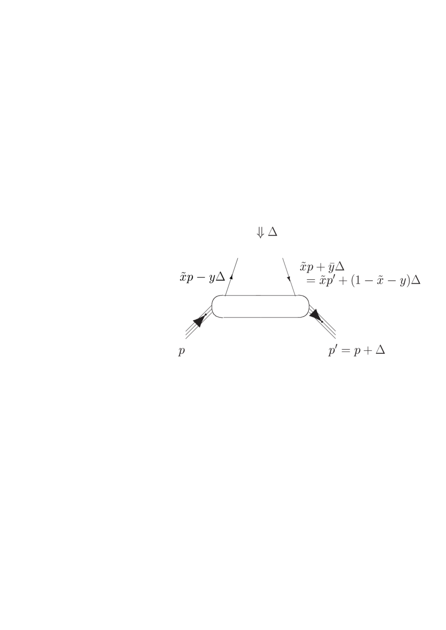
FIG. 3.: Diagram to denote the arguments $\tilde{x}$, $y$ and $\Delta^{2}$ of the double distributions.

FIG. 4.: Factorization for the leading order hard meson electroproduction amplitude.

FIG. 5.: $\xi$ dependence of the OFPD $H^{d}$ at $t=0$ using the ansatz (based on the MRST98 [17] quark distributions) as described in the text. Upper panel : valence down quark OFPD, lower panel : total down quark OFPD. The thin lines ($\xi=0$) correspond with the ordinary $d$-quark distributions (MRST98 parametrization at $Q^{2}$ = 2 GeV²).

FIG. 6.: Leading order diagrams to hard meson electroproduction.

FIG. 7.: Leading order direct (a) and crossed (b) diagrams to the $\pi^{0}\gamma^{*}\gamma$ transition form factor.

FIG. 8.: Results for the $\pi^{0}\gamma^{*}\gamma$ transition form factor of the leading order PQCD prediction (dashed-dotted line) compared with the prediction including transverse momentum dependence (full line). Data are from CELLO [39] and CLEO [30].

FIG. 9.: Impact parameter (b) dependence of the OFPD $H^{d}_{V}$ for the valence down quark, using the model ansatz (based on the MRST98 quark distributions) as described in the text.

FIG. 10.: Leading order direct (a) and crossed (b) diagrams to the $\pi$ electromagnetic form factor involving one-gluon exchange. Soft overlap contribution (c) to the $\pi$ form factor. There are analogous diagrams where the virtual photon couples to the lower quark line, which are not shown here.

FIG. 11.: Results for the $\pi$ electromagnetic form factor of the leading order PQCD prediction without (dotted line) and with (dashed-dotted line ) inclusion of the corrections due to intrinsic transverse momentum dependence. The dashed curve shows the result for the soft overlap contribution of Fig. 10c and the total result (full line) is the sum of the dashed and dashed-dotted lines. The “data” points from Refs.[44] (CEA) and [45] (Cornell) were obtained indirectly from pion electroproduction.

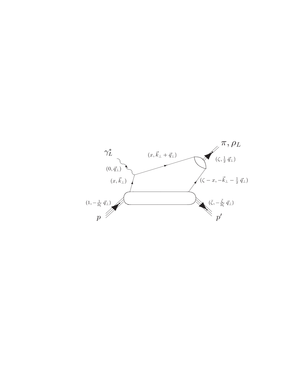
FIG. 12.: Soft overlap contribution to the meson electroproduction amplitude.

FIG. 13.: Comparison between the angular dependence of the leading order predictions for the $\rho^{0}_{L}$ (full lines), $\pi^{+}$ (thick, upper dashed lines) leptoproduction and DVCS (thick dotted lines) in-plane cross sections at $Q^{2}$ = 2.5 GeV², $x_{B}$ = 0.3 and for different beam energies : $E_{\mu^{+}}$ = 200 GeV (COMPASS), $E_{e^{+}}$ = 27 GeV (HERMES), $E_{e^{-}}$ = 6 GeV (JLab). The BH (thin dotted lines) and total $\gamma$ (dashed-dotted lines) cross sections are also shown. For the $\pi^{+}$, the result excluding the pion pole is also shown (thin, lower dashed lines).

FIG. 14.: Angular dependence of the leading order amplitudes for $\rho^{0}_{L}$ leptoproduction at $E_{\mu}$ = 200 GeV, $Q^{2}$ = 2.5 GeV², and for different values of $x_{B}$. The prediction with a $\xi$-dependent ansatz for the OFPD’s (full lines) are compared with a $\xi$-independent ansatz for the OFPD’s (dashed-dotted lines).

FIG. 15.: DVCS at JLab for out-of-plane kinematics ($\phi=120^{o}$). Upper part shows the differential cross section : DVCS including the $\pi^{0}$ pole contribution (dashed line), BH (dotted line), total $\gamma$ excluding the $\pi^{0}$ pole contribution (dashed-dotted line) and total $\gamma$ including the $\pi^{0}$ pole contribution (full line). In the lower part, the electron single spin asymmetry is shown for the L.O. DVCS amplitude (calculated in radiative gauge) excluding the $\pi^{0}$ pole (dashed line) and including the $\pi^{0}$ pole (full line). We also show the result for the gauge invariant DVCS amplitude, excluding the $\pi^{0}$ pole (dashed-dotted line).

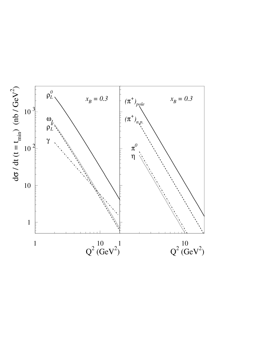
FIG. 16.: Scaling behavior of the leading order predictions for the forward differential electroproduction cross section $d\sigma_{L}/dt$ on the proton, for vector mesons (left panel) and pseudoscalar mesons (right panel) using a coupling constant frozen at a scale 1 GeV². For the $\pi^{+}$ channel, the pion pole contribution (full line, $(\pi^{+})_{pole}$) is shown separately from the $\tilde{H}$ contribution (dashed line, $(\pi^{+})_{n.p.}$). Also shown is the scaling behavior of the forward transverse cross section $d\sigma_{T}/dt$ for the leading order DVCS cross section (dashed-dotted line in left panel).

FIG. 17.: DVCS transverse cross section $d\sigma_{T}/dt$ (multiplied with the scaling factor $Q^{4}$) in the forward direction ($t=t_{min}$). The leading order result is given by the dashed-dotted line and the result including the intrinsic transverse momentum dependence is given by the full line.

FIG. 18.: Longitudinal differential cross section $d\sigma_{L}/dt$ in the forward direction ($t=t_{min}$) for for $\gamma^{*}_{L}p\longrightarrow\rho^{0}_{L}p$ . The leading order result is given by the dashed line and the result including the intrinsic transverse momentum dependence is given by the full line. The calculation of the soft overlap contribution is given by the dashed-dotted line.

FIG. 19.: Longitudinal forward differential cross section for $\rho^{0}_{L}$ electroproduction. Calculations compare the quark exchange mechanism (dotted lines) with the two-gluon exchange mechanism (dashed lines) and the sum of both (full lines). Both calculations include the corrections due to intrinsic transverse momentum dependence as described in the text. The data are from NMC (triangles) [49], E665 (solid circles) [50], ZEUS 93 (open circles) [51] and ZEUS 95 (open squares) [52].

FIG. 20.: Longitudinal forward differential cross section for $\rho^{0}_{L}$ electroproduction. Calculations show the sum of the quark exchange and two-gluon exchange mechanisms for different values of $Q^{2}$ (in GeV²) as indicated on the curves. The data are from NMC [49], E665 [50], ZEUS 93 [51] and ZEUS 95 [52].

FIG. 21.: $Q^{2}$-dependence for the longitudinal forward differential electroproduction cross section $d\sigma_{L}/dt$ for $\gamma^{*}p\rightarrow\pi^{+}n$ at $x_{B}=0.24$. The leading order pion pole contribution (dotted line) and $\tilde{H}$ contribution (dashed-dotted line) are shown using a running coupling constant with $\Lambda_{QCD}$ = 0.2 GeV. Also shown (dashed line) is the calculation including the power corrections to the pion pole contribution (intrinsic transverse momentum dependence and overlap contribution to the pion FF), as well as the sum of the pion pole and $\tilde{H}$ contribution including the power corrections (full line). The data are from Ref. [45] : the points at $Q^{2}$ = 1.2 and 2.0 GeV² correspond with $x_{B}\approx 0.24$, whereas the point at $Q^{2}$ = 3.3 GeV² corresponds with $x_{B}\approx 0.35$.

REFERENCES

- [1] X. Ji, Phys. Rev. Lett. 78, 610 (1997); Phys. Rev. D 55, 7114 (1997).
- [2] A.V. Radyushkin, Phys. Lett. B 380, 417 (1996); Phys. Rev. D 56, 5524 (1997).
- [3] A.V. Radyushkin, Phys. Lett. B 385, 333 (1996).
- [4] J.C. Collins, L. Frankfurt and M. Strikman, Phys. Rev. D 56, 2982 (1997).
- [5] M. Vanderhaeghen, P.A.M. Guichon and M. Guidal, Phys. Rev. Lett. 80, 5064 (1998).
- [6] P.A.M. Guichon and M. Vanderhaeghen, Prog. Part. Nucl. Phys. 41, 125 (1998).
- [7] JLab experiment E98-107 : “Deeply Virtual Electroproduction of Vector Mesons”; spokespersons M. Guidal, C. Marchand and E. Smith.
- [8] P.Y. Bertin, C. Hyde-Wright and Y. Roblin, Proceedings of the conference “Nuclear and Particle Physics with CEBAF at JLAB”, Dubrovnik, 1998.
- [9] G. Leibbrandt, Rev. Mod. Phys. 59, 1067 (1987).
- [10] P. Hoodbhoy and X. Ji, Phys. Rev. D 58, 054006 (1998).
- [11] X. Ji, J. Phys. G 24, 1181 (1998).
- [12] M. Diehl, T. Gousset and B. Pire, Phys. Rev. D 59, 034023 (1999).
- [13] R.L. Jaffe, “Spin, Twist and Hadron Structure in Deep Inelastic Processes, Lectures presented at the 1995 Erice Summer School on the Spin Structure of the Nucleon”, in Lectures on QCD, 178-249, Ed. F.Lenz.
- [14] A.V. Radyushkin, Phys. Rev. D 59, 014030 (1999); Phys. Lett. B 449, 81 (1999).
- [15] Particle Data Group, C. Caso et al., Eur. Phys. J. C 3, 1 (1998).
- [16] E. Leader, A.V. Sidorov and D.B. Stamenov, Phys. Rev. D 58, 114028 (1998).
- [17] A.D. Martin, R.G. Roberts, W.J. Stirling, R.S. Thorne, Eur. Phys. J. C 4, 463 (1998).
- [18] L.L. Frankfurt, M.V. Polyakov and M. Strikman, hep-ph/9808449, in Proceedings of the Workshop “Jefferson Lab Physics and Instrumentation with 6-12-GeV Beams”; Eds. S. Dytman, H. Fenker and P. Roos (Newport News, 1998).
- [19] L.L. Frankfurt, P.V. Pobylitsa, M.V. Polyakov and M. Strikman, hep-ph/9901429.
- [20] X. Ji, W. Melnitchouk and X. Song, Phys. Rev. D 56, 5511 (1997).
- [21] V. Petrov, P. Pobylitsa, M. Polyakov, I. Börnig, K. Goeke, C. Weiss, Phys. Rev. D 57, 4325 (1998).
- [22] M.V. Polyakov and C. Weiss, hep-ph/9902451.
- [23] I.I. Balitsky and X. Ji, Phys. Rev. Lett. 79, 1225 (1997).
- [24] B. Adeva et al. (SMC Collaboration), Phys. Lett. B 420, 180 (1998).
- [25] X. Ji and J. Osborne, Phys. Rev. D 58, 094018 (1998).
- [26] J.C. Collins and A. Freund, Phys. Rev. D 59, 074009 (1999).
- [27] L. Mankiewicz, G. Piller, T. Weigl, Eur. Phys. J. C 5, 119 (1998);
- [28] L. Mankiewicz, G. Piller, T. Weigl, Phys. Rev. D 59, 017501 (1999).
- [29] L. Mankiewicz, G. Piller and A. Radyushkin, hep-ph/9812467.
- [30] J. Gronberg et al. (CLEO Collaboration), Phys. Rev. D 57, 33 (1998).
- [31] P. Ball and V.M. Braun, Phys. Rev. D 54, 2182 (1996); hep-ph/9808229.
- [32] A.P. Bakulev and S.V. Mikhailov, Phys. Lett. B 436, 351 (1998).
- [33] M. Polyakov, hep-ph/9809483.
- [34] I.V. Musatov and A.V. Radyushkin, Phys. Rev. D 56, 2713 (1997).
- [35] R. Jakob, P. Kroll and M. Raulfs, J. Phys. G 22, 45 (1996); P. Kroll and M. Raulfs, Phys. Lett. B 387, 848 (1996).
- [36] J. Botts and G. Sterman, Nucl. Phys. B 325, 62 (1989); H.N. Li and G. Sterman, Nucl. Phys. B 381, 129 (1992).
- [37] S.J. Brodsky and G.P. Lepage in Perturbative QCD, edited by A.H. Mueller (World Scientific, Singapore, 1989).
- [38] S.J. Brodsky, T. Huang and G.P. Lepage, in Particles and Fields 2, Proceedings of the Banff Summer Institute, Banff, Canada, 1981; eds. A. Capri and A. Kamal (Plenum, New York, 1983), p.143.
- [39] H.-J. Behrend et al. (CELLO Collaboration), Z. Phys. C 49, 401 (1991).
- [40] H.N. Li, Phys. Rev. D 48, 4243 (1994).
- [41] N.G. Stefanis and W. Schroers, H.-Ch. Kim, Phys. Lett. B 449, 299 (1999); hep-ph/9812280.
- [42] D.V. Shirkov and I.L. Solovtsov, Phys. Rev. Lett. 79, 1209 (1997).
- [43] K.A. Milton and I.L. Solovtsov, Phys. Rev. D 55, 5295 (1997).
- [44] C.N. Brown et al., Phys. Rev. D 8, 92 (1973).
- [45] C.J. Bebek et al., Phys. Rev. D 17, 1693 (1978).
- [46] M. Sawicki, Phys. Rev. D 46, 474 (1992).
- [47] S.D. Drell and T.M. Yan, Phys. Rev. Lett. 24, 181 (1970).
- [48] L. Frankfurt, W. Koepf and M. Strikman, Phys. Rev. D 54, 3194 (1996).
- [49] M. Arneodo et al. (NMC Collaboration), Nucl. Phys. B 429, 503 (1994).
- [50] M.R. Adams et al. (E665 Collaboration), Z. Phys. C 74, 237 (1997).
- [51] M. Derrick et al. (ZEUS Collaboration), Phys. Lett. B 356, 601 (1995).
- [52] J. Breitweg et al. (ZEUS Collaboration), Eur. Phys. J. C 6, 603 (1999).