UT-841
Critical Exponents of O(N) Scalar Model at Temperatures below the Critical Value using Auxiliary Mass Method

Abstract

We investigate a phase transition of the O(N) invariant scalar model using the auxiliary mass method. We determine the critical exponent $\beta$ by calculating an effective potential below the critical temperature. This work follows that of a previous paper.[1]

Phase transitions at finite temperature are important phenomena in particle physics, cosmology and condensed matter physics. For example, the QGP phase is produced in heavy ion collisions.[2] Some phase transitions occured in the early universe.[3] The electro-weak phase transition in particular plays an important role in the electro-weak baryogenesis scenario[4] and gives some constraints to models of elementary particle physics.[5, 6, 7]  We also see a great number of phase transitions in condensed matter physics. In the present paper, we investigate an O(N) invariant scalar model which corresponds to many condensed matter systems, for example alloys, superfluids, and binary liquids.[8]

To investigate such phase transitions, we can use finite temperature field theory, which is based only on a statistical principle. However, we often have an infrared divergence and cannot obtain reliable results using perturbation theory at finite temperature.[9] To overcome this problem, we used the auxiliary-mass method,[10, 11, 12] and calculated an effective potential and critical exponents of the O(N) invariant scalar model above the critical temperature $T_{c}$ in a previous paper.[1]  We did not investigate at a temperature below $T_{c}$ for two reasons, numerical instability and the lack of computer power. In this work we have overcome these problems, and we calculate an effective potential and critical exponents of the O(N) invariant scalar model below the critical temperature.

We explain the idea of the auxililary-mass method. Since we can calculate a reliable effective potential for temperatures $T\ll\frac{m}{\lambda}$ using perturbation theory,[9] first we assume the mass as $m\sim T$ and calculate an effective potential. This potential is reliable if the coupling constant, $\lambda$, is small. We next extrapolate the effective potential to that of a true mass using a non-perturbative evolution equation. Finally, we determine the necessary physical quantities. We determine critical exponents below $T_{c}$ in the present paper.

Applying this method to the O(N) invariant scalar model, the Euclidean Lagrangian density is given by

$${\cal L}_{E}=-\frac{1}{2}\left(\frac{\partial\phi_{a}}{\partial\tau}\right)^{2}-\frac{1}{2}(\mbox{\boldmath$\nabla$}\phi_{a})^{2}-\frac{1}{2}m^{2}\phi_{a}^{2}-\frac{\lambda}{4!}(\phi_{a}^{2})^{2}+J_{a}\phi_{a}+c.t.\$$ (1)

Here, the $J_{a}$ are external source functions, and the index $a$ runs from 1 to N. We assume that the coupling constant $\lambda$ is small, and therefore the perturbation theory at zero temperature is reliable. We first calculate the effective potential at an auxiliary large mass $m=M\sim T$ at the one-loop level as

$$V = \frac{1}{2}M^{2}\bar{\phi}^{2}+\frac{\lambda}{4!}\bar{\phi}^{4}+\frac{T}{2\pi^{2}}\int^{\infty}_{0}dr\ r^{2}\log\left[1-\exp\left(-\frac{1}{T}\sqrt{r^{2}+M^{2}+\frac{\lambda}{2}\bar{\phi}^{2}}\right)\right]$$ (2)

$$+(N-1)\ \frac{T}{2\pi^{2}}\int^{\infty}_{0}dr\ r^{2}\log\left[1-\exp\left(-\frac{1}{T}\sqrt{r^{2}+M^{2}+\frac{\lambda}{6}\bar{\phi}^{2}}\right)\right].$$

Here $\bar{\phi}$ is a field expectation value. We leave only the finite-temperature part of the equation because we can ignore the zero temperature part due to the small coupling constant. We note that the daisy-resummation is not necessary because of the large mass. We then construct a non-perturbative evolution equation which connects the effective potential at an auxiliary large mass, $m^{2}\sim T^{2}$, and that of the true mass, $m^{2}=-\mu^{2}$. Since we have constructed this for the O(N) invariant scalar model in a previous work,[1] we present only the result:

$$\frac{\partial V}{\partial m^{2}} = \frac{1}{2}\bar{\phi}^{2}+\frac{1}{4\pi^{2}}\int^{\infty}_{0}dr\ r^{2}\frac{1}{\displaystyle\sqrt{r^{2}+\frac{\partial^{2}V}{\partial\bar{\phi}^{2}}}}\frac{1}{\displaystyle\exp\left(\frac{1}{T}\sqrt{r^{2}+\frac{\partial^{2}V}{\partial\bar{\phi}^{2}}}\right)-1}$$ (3)

$$+\frac{N-1}{4\pi^{2}}\int^{\infty}_{0}dr\ r^{2}\frac{1}{\displaystyle\sqrt{r^{2}+\frac{1}{\bar{\phi}}\frac{\partial V}{\partial\bar{\phi}}}}\frac{1}{\displaystyle\exp\left(\frac{1}{T}\sqrt{r^{2}+\frac{1}{\bar{\phi}}\frac{\partial V}{\partial\bar{\phi}}}\right)-1}.$$

This partial differential equation is solved with the initial conditions (2) numerically.

We display the effective potential for N=4 around $T_{c}$ in Fig. 1, and we find that the phase transition is of second order. The same behaviour is found for other values of N. This is consistent with other analyses using lattice field theory and renormalization group theory.[8] We find that the auxiliary-mass method satisfactorily deals with the problem of the infrared divergence.

\begin{picture}(16.0,8.0)\centerline{\hbox{ \epsfbox{Onfinalpot.eps} }} \end{picture}

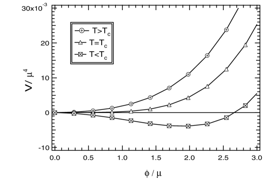
Figure 1: The effective potential obtained by the auxiliary-mass method ($N=4,\lambda=0.01$). A second-order phase transition occurs at the critical temperature. Similar behaviour is observed at other values of N and $\lambda$.

\begin{picture}(16.0,8.0)\centerline{\hbox{ \epsfbox{Onfinalxmin.eps} }} \end{picture}

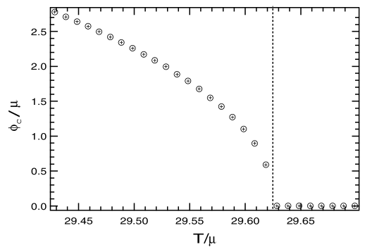
Figure 2: Stable field expectation value $\phi_{c}$ as a function of the temperature $T$ ($\lambda=0.01$). $\phi_{c}$ decreases monotonically and vanishes smoothly as the temperature increases.

\begin{picture}(16.0,8.0)\centerline{\hbox{ \epsfbox{Onfinalfit.eps} }} \end{picture}

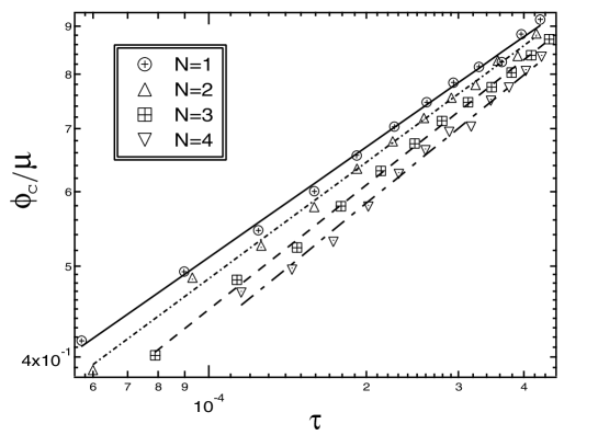
Figure 3: Log-scale plots of $\phi_{c}-\tau$ ($\lambda=0.01$). The data were fit by linear functions with gradients corresponding to $\beta$ for each N. We find that the exponent $\beta$ is larger for larger N.

We next determine the critical exponents and study how well the auxiliary-mass method works. Since we have investigated this model above $T_{c}$ previously, obtainig the critical exponents $\gamma$ and $\delta$,[1] we investigate below $T_{c}$ and determine the critical exponent $\beta$ here. The critical exponent, $\beta$ relates an order parameter, $\phi_{c}$, to a reduced temperature, $\tau\equiv\frac{T_{c}-T}{T_{c}}$, as

$$\phi_{c}\propto\tau^{\beta}.$$ (4)

The order parameter $\phi_{c}$ as a function of reduced temperature $\tau$ is presented in Fig.2 for N=4. Similar behaviour for other values of N is found. Since the order parameter $\phi_{c}$ vanishes smoothly at $T_{c}$, we find that the phase transition is of second order. We next plot $\phi_{c}$ as a function of $\tau$ in Fig.3 for various N. These data appear linear with different gradients, corresponding to $\beta$ for each N. The exponent, $\beta$ is larger for larger values of N.

We summarise the results of a present paper and a previous paper[1] in Table.1. The values of $\beta,\gamma$ and $\delta$ are much better than the Landau approximation and the dependence on N is close to the most reliable value (MRV). There are, however, slight differences between our results and the MRV, which are caused by an approximation in deriving Eq.3.

In conclusion, we have investigated the O(N) invariant scalar model using the auxiliary-mass method and have obtained good results both qualitatively and quantitatively. These results suggest that the auxiliary-mass method is an effective tool at finite temperature. We were able to investigate not only second order phase transitions but also first order phase transitions since the finite-temperature field theory is based only on a statistical principle. We therefore believe that this is one of the most powerful methods to investigate a weak first order phase transition and models which have end-points : cubic anisotropy, the abelian Higgs model and the standard model.

Table 1: The critical exponents $\beta$, $\gamma$ and $\delta$ obtained in a present paper and the previous paper. Those of Landau approximation (LA) and the most reliable values (MRV) are also summarised. We used the results of the six-loop approximation using the Padé-Borel resummation for the MRV here.

	$\beta$ (LA,MRV)	$\gamma$ (LA,MRV)	$\delta$ (LA,MRV)
N$=$1 [13]	0.39 (0.5, 0.327)	1.37 (1, 1.239)	4.0 (3, 4.8)
N$=$2 [13]	0.41 (0.5, 0.348)	1.47 (1, 1.315)	4.2 (3, 4.8)
N$=$3 [13]	0.44 (0.5, 0.366)	1.60 (1, 1.386)	4.4 (3, 4.8)
N$=$4 [13]	0.45 (0.5, 0.382)	1.66 (1, 1.449)	4.4 (3, 4.8)

The authors are supported by JSPS fellowship.

References

- [1] K. Ogure and J. Sato \PRD58,1998,085010.
- [2] M. Le. Bellac, Thermal Field Theory (Cambridge Univ. Press, 1996).
- [3] E. W. Kolb and M. S.Turner, The Erly Universe (Addison-Wesley, New York, 1990).
- [4] V. Kuzmin, V. Rubakov and M. E. Shaposhnikov,\PLB155,1985,36.
- [5] A. G. Cohen, D. B. Kaplan and A. E. Nelson Ann. Rev. Nucl. Part. Sci. 43 (1993) 27.
- [6] V. A. Rubakov and M. E. Shaposhnikov Usp.Fiz.Nauk 166 (1996) 493, Phys.Usp. 39 (1996) 461, hep-th/9603208.
- [7] M. Carena, M. Quiros, C.E.M. Wagner \NPB524,1998,3.
- [8] J. Zinn-Justin, Quantum Field Theory and Critical Phenomena, (Oxford Univ. Press, New York, 1996).
- [9] P. Fendley,\PLB196,1987,175.
- [10] I. T. Drummond, R. R. Horgan, P. V. Landshoff and A. Rebhan, \PLB398,1997,326 .
- [11] T.Inagaki, K.Ogure and J.Sato,\PTP99,1998,1069.
- [12] K.Ogure and J.Sato,\PRD57,1998,7460.
- [13] S.A.Antonenko and A.I.Sokolov \PRE51,1995,1984.