Multiplicity Fluctuations
in One- and Two-Dimensional Angular Intervals
Compared with Analytic QCD Calculations

DELPHI Collaboration
B. Buschbeck and F. Mandl

Institute for High Energy Physics of the Austrian Academy of Sciences, Vienna, Austria

Multiplicity fluctuations in rings around the jet axis and in off-axis cones have been measured by the DELPHI collaboration in $e^{+}e^{-}$ annihilations into hadrons at LEP energies. The measurements are compared with analytical perturbative QCD calculations for the corresponding multiparton system, using the concept of Local Parton Hadron Duality. Some qualitative features are confirmed by the data but substantial quantitative deviations are observed.

1 Introduction

To describe multiplicity fluctuations in angular regions by analytical calculations using perturbative QCD is a challenge. It could help to improve our understanding of the parton cascading mechanism and might lead to a simple description of multiparticle correlations by QCD alone. The idea that QCD jets might exhibit a self-similar (or fractal) structure was brought up already in 1979 by R.P.Feynman [1], A.Giovannini [2] and G.Veneziano [3]. In recent years this conception has been confirmed by various groups [4, 5, 6], giving detailed predictions on variables and phase space regions where fractality is expected to show up. A simple predicted dependence of the fractal dimensions on $\alpha_{s}$ stimulated further interest in measuring them experimentally.

The analytical calculations are performed in the Double Log Approximation (DLA) [7, 8], neglecting energy-momentum conservation, and concern only idealized jets. They provide leading order predictions applicable quantitatively at very high energies ( $\geq$ 1 TeV) [4]. At LEP energies, non-perturbative effects may be important. Also, they refer to multiparton states, whereas only multihadron states can be measured. It has been suggested that the parton evolution should be extended from the perturbative regime down to a lower mass scale (if possible to the mass scale of light hadrons) to be able to compare the partonic states directly with the hadronic states. This concept of Local Parton Hadron Duality (LPHD) [9] is quite successful for single particle distributions and for global moments of multiplicity distributions. It remains questionable in the case of the more refined variables used here, namely factorial moments and cumulants in phase space bins. First experimental measurements [10, 11, 12, 13, 14] revealed, indeed, substantial deviations.

On the other hand it can be expected that these calculations will improve in the future. This would provide us with a better understanding of the internal structure of jets in terms of analytical expressions than can be obtained by Monte Carlo calculations with many parameters. In fact, the analytical predictions considered in this paper involve only one adjustable parameter, namely the QCD scale $\Lambda$.

The aim of this study is to use DELPHI data to measure multiplicity fluctuations in one- and two-dimensional angular intervals and compare them with the available theoretical predictions. It is hoped that such a study may show how to approach nearer to a satisfying theory based on QCD and LPHD which describes high energy multiparticle phenomena.

In section 2 the theoretical framework is sketched, section 3 contains information about the experimental data and the Monte Carlo comparisons and in section 4 the comparison with the analytical calculations is presented. Section 5 contains the final discussion and the summary.

2 Theoretical framework

The theoretical calculations treat correlations between partons emitted within an angular window defined by two angles $\vartheta$ and $\Theta$. The parton and particle density correlations (fluctuations) in this window are described by normalized factorial moments of order $n$:

$$F^{(n)}(\Theta,\vartheta)=\frac{\int\rho^{(n)}(\Omega_{1},\ldots,\Omega_{n})d\Omega_{1}\ldots d\Omega_{n}}{\int\rho^{(1)}(\Omega_{1})\ldots\rho^{(1)}(\Omega_{n})d\Omega_{1}\ldots d\Omega_{n}}$$ (1)

where $\rho^{(n)}(\Omega_{1},\ldots,\Omega_{n})$ are the $n$-parton/particle density correlation functions which depend on the spherical angles $\Omega_{k}$. The integrals extend over the window chosen.

The angular windows considered here are either rings around the jet axis with mean opening angle $\Theta=25^{\circ}$ and half width $\vartheta$ in the case of 1 dimension ($D=1$), or cones with half opening angle $\vartheta$ around a direction ($\Theta,\Phi$) with respect to the jet axis in the case of 2 dimensions ($D=2$). At sufficiently large jet energies, the parton flow in these angular windows is dominated by parton avalanches caused by gluon bremsstrahlung off the initial quark.

The cumulants $C^{(n)}$ are obtained from the moments $F^{(n)}$ by simple algebraic equations [15], e.g. $C^{(2)}=F^{(2)}-1$, $C^{(3)}=F^{(3)}-3(F^{(2)}-1)-1$ .

The theoretical scheme for deriving the moments described above is based on the generating functional techniques [8, 16] in the DLA of perturbative QCD. The probability of radiating a gluon with momentum $k$ at an emission angle $\Theta_{g}$ and azimuthal angle $\Phi_{g}$ from an initial parton $a$ has been approximated by

$$M(k)d^{3}k=c_{a}\gamma_{0}^{2}\frac{dk}{k}\frac{d\Theta_{g}}{\Theta_{g}}\frac{d\Phi_{g}}{2\pi}$$ (2)

$$\gamma_{0}^{2}=6\alpha_{S}/\pi$$ (3)

with $c_{a}$ = 1 if $a$ is a gluon and $c_{a}$ = 4/9 if $a$ is a quark.

Ref. [4] derived their predictions explicitly for cumulant moments $C^{(n)}$, whereas [5] and [6] obtained similar expressions for the factorial moments $F^{(n)}$. It has been shown [4] by Monte Carlo calculations that, at very high energy ($\sqrt{s}\geq 1800$ GeV), the values of $F^{(n)}$ and $C^{(n)}$ converge to each other. At LEP energies, however, the cumulants are still far away from the asymptotic predictions (see section 4).

For the normalized cumulant moments $C^{(n)}$ [4] and the factorial moments $F^{(n)}$ [5, 6], the following prediction has been made:

$$C^{(n)}(\Theta,\vartheta)~{}\mbox{or}~{}F^{(n)}(\Theta,\vartheta)\sim\left(\frac{\Theta}{\vartheta}\right)^{\phi_{n}}$$ (4)

All 3 references [4, 5, 6] give in the high energy limit and for large values of $\vartheta\leq\Theta$ the same linear approximation for the exponents $\phi_{n}$:

$$\phi_{n}\approx(n-1)D-\left(n-\frac{1}{n}\right)\gamma_{0}$$ (5)

where D is a dimensional factor, 1 for ring regions and 2 for cones. For fixed $\alpha_{s}$ (along the parton shower) eq. 5 is asymptotically valid for all angles. In this case the fractal (Renyi-) dimension $D_{n}$ [17] can be obtained [18] from $\phi_{n}$ (eq. 5) via:

$$D_{n}=D-\frac{\phi_{n}}{n-1}$$ (6)

$$D_{n}=\frac{n+1}{n}\gamma_{0}$$ (7)

When the running of $\alpha_{S}$ with $\vartheta$ in the parton cascade is taken into account, in [4] the following was obtained

$$\phi_{n}\approx(n-1)D-2\gamma_{0}(n-\omega(\epsilon,n))/\epsilon$$ (8)

$$\omega(\epsilon,n)=n\sqrt{1-\epsilon}(1-\frac{1}{2n^{2}}\ln(1-\epsilon))$$ (9)

and

$$\epsilon=\frac{\ln(\Theta/\vartheta)}{\ln(P\Theta/\Lambda)}$$ (10)

where $P\approx\sqrt{s}/2$ is the momentum of the initial parton. The dependence on the QCD parameters $\alpha_{s}$ or $\Lambda$ enters in the above equations via $\gamma_{0}$ and $\epsilon$ that are determined by the scale $Q\approx P\Theta$. In the present study it is about 20 GeV for $\sqrt{s}$=91.1 GeV.

The corresponding predictions of refs. [5] (eq. 11) and [6] (eq. 12) are analytically different, but numerically similar:

$$\phi_{n}=(n-1)D-\frac{2\gamma_{0}}{\epsilon}\cdot\frac{n^{2}-1}{n}\left(1-\sqrt{1-\epsilon}\right)$$ (11)

$$\phi_{n}=(n-1)D-\frac{n^{2}-1}{n}\gamma_{0}\left(1+\frac{n^{2}+1}{4n^{2}}\epsilon\right)$$ (12)

It should be noted that all three theoretical papers cited above use the lowest order QCD relation (13) between the coupling $\alpha_{s}$ and the QCD scale $\Lambda$, which is also used in the present analysis:

$$\alpha_{s}=\frac{\pi\beta^{2}}{6}\frac{1}{\ln(Q/\Lambda)}$$ (13)

$$\beta^{2}=12\left(\frac{11}{3}n_{c}-\frac{2}{3}n_{f}\right)^{-1}$$ (14)

where $n_{c}$=3 (number of colours). These relations depend also on the number of flavours ($n_{f}$). Since eq. 13 emerges only from “one loop” calculations, the parameter $\Lambda$ is not the universal $\Lambda_{\overline{MS}}$, but only an effective parameter $\Lambda_{eff}$. But also in this approximation $\alpha_{s}$ runs, having a scale dependence $1/\ln(Q^{2}/\Lambda^{2})$.

The running of $\alpha_{s}$ during the process of jet cascading is implicitly taken into account in (8), (11) and (12) by the dependence of $\phi_{n}$ on $\epsilon$ (or $\vartheta$). In theory this causes a deviation from a potential behaviour (eqs. 4 and 5) of $F^{(n)}$ when approaching smaller values of $\vartheta$ (larger $\epsilon$).

All theoretical predictions concern the partonic states. The corresponding experimental measurements, however, are of hadronic states. When comparing them, the hypothesis of LPHD has to be used.

It may be noted that the factorial moments $F^{(n)}$ measured in the present study (see also eq. 15 below) are very similar to the well known and previously measured moments in rapidity space. Here the angle $\vartheta$ is used (translated by constant factors into $\epsilon$), because this is the natural variable in the QCD calculations.

3 Experimental data and comparison with the Monte Carlo calculations

The normalized factorial moments (1) are determined experimentally by counting $n_{m}$, the number of charged particles in the respective windows of phase space, for each event:

$$F^{(n)}(\Theta,\vartheta)=\frac{\left<n_{m}(n_{m}-1)\ldots(n_{m}-n+1)\right>}{\left<n_{m}\right>^{n}}$$ (15)

where the brackets $<>$ denote averages over the whole event sample.

The data sample used contains about 600000 $e^{+}e^{-}$ interactions (after cuts) collected by DELPHI at $\sqrt{s}=91.1$ GeV in 1994. A sample of about 1200 high energy events at $\sqrt{s}$=183 GeV incident energy collected in 1997 is used to investigate the energy dependence. The calculated hadron energy was required to be greater than 162 GeV (corresponding to a mean energy of 175 GeV). The standard cuts as in [19] for hadronic events and track quality were applied by demanding a minimum charged multiplicity, enough visible charged energy and events well contained within the detector volume. In the present study all charged particles (except identified electrons and muons) with momentum larger than 0.1 GeV have been considered. The special procedures for selecting high energy events are described in [20]. WW-events have been excluded. Detailed Monte Carlo studies were done using the JETSET 7.4 PS model [21]. The corrections were determined using events from a JETSET Monte Carlo simulation which had been tuned ($\Lambda$=0.346 GeV and $Q_{0}$=2.25 GeV) to reproduce general event characteristics [22], which included variables different from those referred to in section 2. These events were examined at

• Generator level
  where all charged final–state particles (except electrons and muons) with a mean lifetime longer than $10^{-9}$ seconds have been considered;

• Detector level
  which includes distortions due to particle decays and interactions with the detector material, other imperfections such as limited resolution, multi–track separation and detector acceptance, and the event selection procedures.

Using these events, the factorial moments and cumulants introduced in section 2 of order $n$, $A_{n}$, studied below were corrected (for each $\epsilon$ interval considered) by

$$A^{\rm{cor}}_{n}\,=\,g_{n}A^{\rm{raw}}_{n}\,,\quad g_{n}\,=\,\frac{A^{\rm{gen}}_{n}}{A^{\rm{det}}_{n}}$$ (16)

where the superscript “raw” indicates the quantities calculated directly from the data, and “gen” and “det” denote those obtained from the Monte Carlo events at generator and detector level respectively. The simulated data at detector level were found to agree satisfactorily with the experimental data. The measurement error on the relative angle $\vartheta_{12}$ between two outgoing particles was determined to be of order $0.5^{\circ}$ (if both tracks had good Vertex Detector hits, even as small as $0.1^{\circ}$). The jet axis is chosen to be the sphericity axis. To increase statistics in the case of the high energy sample the moments (15) have been calculated in both sphericity hemispheres and averaged.

In addition, all phenomena which were not included in the analytical calculations had to be corrected for, namely (i) initial state photon radiation, (ii) Dalitz decays of the $\pi^{0}$, (iii) residual $K^{0}_{s}$ and $\Lambda^{0}$ decays near the vertex, and (iv) the effect of Bose–Einstein correlations. The corrections were estimated, for each $\epsilon$ interval, like $g_{n}$ in eq. 16, by switching the effects on and off. Each of these correction factors were found to be below 10% in the case of factorial moments. The largest corrections have been found in the case of cumulants of higher orders and amounted to 16–25%, depending on the analysis angle.

The total correction factor including all effects is denoted by $g^{\rm{tot}}_{n}$ and is the product of the individual factors. Systematic errors have been calculated from $g^{\rm{tot}}_{n}$ according to $\Delta A^{\rm{corr}}_{n}=\pm|A^{\rm{raw}}_{n}(g^{\rm{tot}}_{n}-1)/2|$. Due to uncertainties in measuring multiple tracks at very small separation angles, an additional systematic error was added for small $\vartheta$ values for $F^{(4)}$ and $F^{(5)}$.

Figure 1: a) The measured ($\bullet$) cumulants of order $n=2$ in 1-D rings, b) those of order $n=3$, c) the factorial moments of orders $n=2$ to 5 in 1-D rings, and d) those in 2-D off-axis cones are compared with JETSET 7.4 before ($\diamond$) and after ($\circ$) resonance decay. The polar angle $\Theta=25^{\circ}$. Only charged hadrons have been considered. Because of a negative $C^{3}(0)$ value in JETSET before resonance decay, no normalization was possible in this case and the corresponding points have therefore been omitted in b). Values of $\vartheta$ which correspond to the respective values of $\epsilon$, with $\Lambda=0.15$ GeV, are also indicated in b).

Fig. 1 shows a comparison at $\sqrt{s}$=91.1 GeV of the measured 1-dimensionel cumulants and 1- and 2-dimensional factorial moments with JETSET 7.4 tuned as described above. The cumulants and factorial moments are normalized by $C^{(n)}(0)$ and $F^{(n)}(0)$ for easy comparison of the measured shapes with the analytical predictions. There is generally good agreement between the Monte Carlo simulation (open circles) and the corrected data (full circles). The study of the influence of the resonance decay shown in Fig. 1 reveals significant effects. Numerical values of the measured and corrected 1- and 2-dimensional factorial moments are given in Tables 1 and 2, respectively, for convenience as function of $\vartheta$/$\Theta$ (the $\epsilon$ dependence follows from eq. 10).

Table 1a : 1-dimensional factorial moments for orders 2 and 3
together with their statistical and systematic errors as function of $\vartheta$/$\Theta$ ($\Theta=25^{\circ}$)
$\vartheta/\Theta$ $F_{2}$ $\pm$ stat $\pm$ syst $F_{3}$ $\pm$ stat $\pm$ syst 1.0000 1.035 0.002 0.009 1.114 0.003 0.030 0.9180 1.063 0.002 0.009 1.196 0.003 0.031 0.8426 1.101 0.002 0.010 1.315 0.004 0.034 0.7735 1.139 0.002 0.010 1.446 0.005 0.037 0.7100 1.176 0.003 0.010 1.577 0.006 0.040 0.6518 1.210 0.003 0.011 1.707 0.007 0.043 0.5983 1.241 0.003 0.011 1.831 0.008 0.045 0.5492 1.269 0.003 0.012 1.949 0.009 0.047 0.5041 1.293 0.004 0.012 2.055 0.010 0.048 0.4628 1.316 0.004 0.013 2.156 0.012 0.050 0.4248 1.335 0.004 0.013 2.246 0.013 0.051 0.3899 1.353 0.004 0.014 2.330 0.014 0.054 0.3579 1.368 0.005 0.015 2.406 0.015 0.057 0.3286 1.382 0.005 0.015 2.474 0.017 0.060 0.3016 1.393 0.005 0.016 2.530 0.018 0.061 0.2769 1.402 0.005 0.016 2.576 0.019 0.064 0.2541 1.409 0.006 0.017 2.612 0.021 0.067 0.2333 1.416 0.006 0.018 2.646 0.022 0.071 0.2141 1.422 0.006 0.018 2.672 0.024 0.073 0.1966 1.428 0.006 0.019 2.699 0.025 0.079 0.1804 1.432 0.007 0.020 2.720 0.027 0.086 0.1656 1.435 0.007 0.020 2.740 0.029 0.092 0.1520 1.437 0.007 0.020 2.751 0.031 0.094 0.1396 1.441 0.008 0.021 2.771 0.033 0.097 0.1281 1.444 0.008 0.022 2.785 0.035 0.104 0.1176 1.448 0.008 0.022 2.797 0.037 0.109 0.1080 1.451 0.009 0.022 2.808 0.040 0.108 0.0991 1.454 0.009 0.022 2.812 0.043 0.106

Table 1b : 1-dimensional factorial moments for orders 4 and 5 )
together with their statistical and systematic errors as function of $\vartheta/\Theta$ ($\Theta=25^{\circ}$)

$\vartheta/\Theta$	$F_{4}$	$\pm$ stat	$\pm$ syst	$F_{5}$	$\pm$ stat	$\pm$ syst
1.0000	1.251	0.005	0.068	1.465	0.010	0.135
0.9180	1.417	0.006	0.076	1.757	0.013	0.160
0.8426	1.681	0.008	0.089	2.270	0.019	0.203
0.7735	1.994	0.011	0.103	2.931	0.028	0.253
0.7100	2.332	0.015	0.116	3.697	0.039	0.307
0.6518	2.689	0.018	0.130	4.568	0.052	0.362
0.5983	3.047	0.022	0.141	5.489	0.067	0.412
0.5492	3.406	0.027	0.152	6.467	0.086	0.461
0.5041	3.745	0.032	0.157	7.440	0.106	0.491
0.4628	4.085	0.038	0.165	8.467	0.130	0.528
0.4248	4.395	0.043	0.173	9.436	0.158	0.573
0.3899	4.694	0.050	0.186	10.403	0.190	0.634
0.3579	4.974	0.056	0.200	11.337	0.220	0.837
0.3286	5.227	0.063	0.211	12.196	0.257	1.200
0.3016	5.438	0.071	0.262	12.931	0.304	1.501
0.2769	5.605	0.079	0.260	13.464	0.347	1.320
0.2541	5.739	0.087	0.261	13.924	0.398	1.508
0.2333	5.855	0.096	0.261	14.286	0.456	1.508
0.2141	5.939	0.105	0.263	14.520	0.508	1.503
0.1966	6.021	0.112	0.299	14.714	0.536	1.521
0.1804	6.113	0.123	0.347	15.125	0.611	1.543
0.1656	6.194	0.134	0.395	15.447	0.679	1.671
0.1520	6.228	0.147	0.402	15.381	0.748	1.633
0.1396	6.292	0.160	0.424	15.493	0.819	1.742
0.1281	6.335	0.176	0.467	15.610	0.942	1.959
0.1176	6.351	0.189	0.510	15.544	1.005	2.333
0.1080	6.361	0.207	0.512	15.485	1.091	2.438
0.0991	6.289	0.219	0.502	14.637	1.122	2.279

Table 2a : 2-dimensional factorial moments for orders 2 and 3

together with their statistical and systematic errors as function of $\vartheta/\Theta$ ($\Theta=25^{\circ}$)
$\vartheta/\Theta$ $F_{2}$ $\pm$ stat $\pm$ syst $F_{3}$ $\pm$ stat $\pm$ syst 1.000 1.046 0.002 0.036 1.155 0.004 0.111 0.918 1.143 0.002 0.041 1.476 0.006 0.145 0.843 1.240 0.003 0.047 1.858 0.010 0.193 0.774 1.337 0.004 0.056 2.296 0.015 0.258 0.710 1.428 0.005 0.067 2.769 0.022 0.338 0.652 1.518 0.006 0.080 3.298 0.031 0.435 0.598 1.602 0.007 0.095 3.863 0.043 0.544 0.549 1.678 0.009 0.112 4.440 0.058 0.660 0.504 1.749 0.010 0.129 5.085 0.077 0.784 0.463 1.822 0.012 0.148 5.821 0.103 0.914 0.425 1.888 0.014 0.167 6.506 0.132 1.021 0.390 1.956 0.017 0.186 7.312 0.171 1.123 0.358 2.011 0.019 0.204 8.067 0.222 1.186 0.329 2.069 0.022 0.221 9.007 0.298 1.240 0.302 2.121 0.026 0.236 9.994 0.398 1.258 0.277 2.188 0.030 0.251 10.985 0.503 1.233

Table 2b : 2-dimensional factorial moments for orders 4 and 5

together with their statistical and systematic errors as function of $\vartheta/\Theta$ ($\Theta=25^{\circ}$)
$\vartheta/\Theta$ $F_{4}$ $\pm$ stat $\pm$ syst $F_{5}$ $\pm$ stat $\pm$ syst 1.000 1.356 0.008 0.250 1.703 0.021 0.508 0.918 2.126 0.018 0.397 3.369 0.056 1.009 0.843 3.234 0.035 0.628 6.343 0.138 1.913 0.774 4.738 0.063 0.963 11.133 0.293 3.368 0.710 6.614 0.107 1.405 18.072 0.575 5.428 0.652 9.046 0.182 1.988 28.813 1.187 8.458 0.598 12.110 0.297 2.706 44.913 2.309 12.622 0.549 15.604 0.467 3.469 65.771 4.404 17.235 0.504 20.094 0.693 4.326 94.370 6.777 22.310 0.463 25.785 1.050 5.206 134.110 11.377 27.410 0.425 31.593 1.505 5.758 179.450 17.935 29.940 0.390 38.817 2.178 6.087 234.930 27.941 29.300 0.358 46.590 3.379 5.895 297.580 53.980 23.620 0.329 58.358 5.432 5.405 419.930 104.740 13.500 0.302 72.636 8.664 4.098 599.320 181.600 16.410 0.277 85.249 11.582 1.647 743.900 235.130 46.850

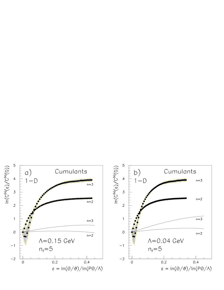
Figure 2: The second and third order cumulants (full circles) are compared with the predictions [4], eq. 8 (solid lines) with $n_{f}=5$ for a) $\Lambda=0.15$ GeV, b) $\Lambda=0.04$ GeV. The statistical errors are shown by the error bars, the systematic errors by the shaded regions.

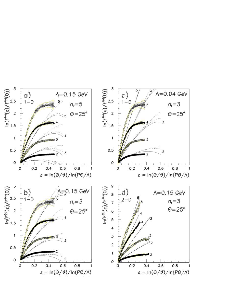
Figure 3: Factorial moments in 1-dimensional rings are compared with the analytical calculations of refs [4, 5, 6], eqs. 8 (solid lines), 11 (dashed lines), and 12 (dotted lines). The dependences on $n_{f}$ and $\Lambda$ are shown in a), b) and c). As a consistency test, 1- and 2-dimensional factorial moments are compared in b) and d) with same QCD parameters: note the different vertical scales. The orders 2 to 5 are indicated in all figures, the data are also distinguished by different symbols. The statistical errors are shown by the error bars, the shaded regions indicate the systematic errors. The 1-dimensional factorial moments agree very well with those measured by L3 [13].

4 Comparison with the analytical calculations

4.1 Quantitative comparison at $\sqrt{s}$ = 91.1 GeV

Fig. 2 shows the cumulants of orders $n$ = 2 and $n$ = 3 in one-dimensional rings around jet cones normalized by $C^{(n)}(0)$ and compared with the predictions of ref. [4].

• The agreement with the data is very bad: The predictions lie well below the data and differ in shape (Fig. 2a). Using a lower value of $\Lambda$ (i.e. $\Lambda=0.04$ GeV instead of 0.15 GeV) does not help, as can be seen in Fig. 2b (neither does a smaller value of $n_{f}$, not shown here).

Fig. 3 shows the factorial moments of orders 2, 3, 4 and 5 normalized by $F^{(n)}(0)$, together with the predictions of refs. [4, 5, 6], in one- and two- dimensional angular intervals (i.e. rings and side cones) for various numerical values of $\Lambda$ and $n_{f}$.

• The correlations in one-dimensional rings around jets, expressed by factorial moments, are not described well by the theoretical predictions [4, 5, 6] using the QCD parameters $\Lambda=0.15$ GeV and $n_{f}=5$ (Fig. 3a). The predictions lie below the data for not too large $\epsilon$, differing also in shape.

• Choosing $n_{f}=3$ (Fig. 3b) instead of $n_{f}=5$ as in Fig. 3a reduces the discrepancies.

• Choosing in addition the smaller value of $\Lambda=0.04$ GeV (Fig. 3c), $F^{(2)}$ is well predicted for smaller values of $\epsilon$, the higher orders ($n>2$) still deviate considerably.

• The factorial moments in 1 and 2 dimensions show different behaviour for the lower order moments $n<4$ : choosing the same set of parameters ($\Lambda=0.15$ GeV, $n_{f}=3$), $F^{(2)}$ and $F^{(3)}$ lie above the predictions in the 1-dimensional case (Fig. 3b), but below them in the 2-dimensional case (Fig. 3d).

• The higher moments $F^{(4)}$ and $F^{(5)}$ have similar features in the 1- and 2-dimensional case (Figs. 3b,3d).

• In Fig. 3 the slopes at small $\epsilon$ are generally steeper than predicted (with the exception of $F^{(2)}$ and $F^{(3)}$ in Fig. 3d) and the “bending” begins at smaller values of $\epsilon$.

• It is not possible to find one set of QCD parameters $\Lambda$ and $n_{f}$ which simultaneously minimize the discrepancies between data and predictions for moments of all orders 2,3,4 and 5 in both the 1- and 2-dimensional cases.

4.2 Energy dependence

Fig.4 shows a comparison with high energy data at $\sqrt{s}$=183 GeV (with a mean energy of $\sqrt{s}$=175 GeV) and the corresponding predictions according to eq. 8, where the energy dependence enters via the parameter $\gamma_{0}$. It can be seen that for small values of $\epsilon$ there is no improvement of agreement at high energy. For larger values of $\epsilon$ the statistical errors of the high energy data are substantial. The relative increase of the predicted moments agrees qualitatively with that of the JETSET model that, as shown in Fig. 1, agrees very well with the measurement at $\sqrt{s}$=91.1 GeV. Similar conclusions can be found from the predictions based on eqs. 11 and 12.

Figure 4: The energy dependence of the normalized factorial moment of order 2. $\sqrt{s}$=91.1 GeV: data (open circles) and prediction ref.[4] dashed lines and $\sqrt{s}$=175 GeV: data (full circles) and prediction ref.[4] solid lines, for the QCD-parameter combinations a) ($n_{f}=3$, $\Lambda$=0.15) and b) ($n_{f}$=3, $\Lambda$=0.04). The full triangles denote the high energy JETSET simulation.

4.3 Qualitative features

In the introduction, arguments have been given that the DLA might not be accurate enough for a quantitative description of experiments. Some disagreement with the measurement could be expected considering the asymptotic nature of the calculations, but nevertheless an overall qualitative description of the data should be provided. Indeed the data (see Figs. 3,4) show some general qualitative features that are predicted well by the analytical calculations:

• The factorial moments rise linearly at small $\epsilon$ exhibiting a fractal structure as predicted in eqs. 4,5 for the parton cascade and saturate at higher values.

• The factorial moments increase from $\sqrt{s}$=91.1 GeV to $\sqrt{s}$=175 GeV.

• The 2-dimensional moments rise much more steeply than the 1-dimensional moments (Figs 3b, 3d).

• The values of $\phi_{n}$ obtained by fitting eq. 4 to the data in the region of small $\epsilon$ ($\epsilon<0.1$) follow the predictions eq. 5 qualitatively, as can be seen in Table 3.

• In Fig. 3 it is shown that the analytically calculated factorial moments depend sensitively on $\Lambda$. It should be noted that a similar dependence (although weaker because of the $\Lambda$-independent fragmentation) is observed in JETSET when varying $\Lambda$ and keeping all other parameters constant.

4.4 Discussion of the QCD parameter $\gamma_{0}$

The first term in the perturbative formula eq. 5 involves the phase space volume, the second one depends explicitly on the parameter $\gamma_{0}$ (eq. 3), i.e. the QCD coupling $\alpha_{s}$. Fig. 5a summarizes the behaviour at small $\epsilon$, where the numerical values of $\gamma_{0}^{eff}$ derived from the measured slopes $\phi_{n}$ are given for the orders $n=2,3,4,5$. From the present theoretical understanding, $\gamma_{0}$ is expected to be independent of $n$. For example, for $\Lambda$=0.15 GeV and $n_{f}$=3 ($\Theta=25^{o}$, $Q\sim P\Theta$) eqs. 13 and 14 give the numerical value $\alpha_{s}$=0.143 and hence from eq. 3 the value $\gamma_{0}$=0.523. This is indicated as horizontal line in Fig. 5, where also the lines for $\Lambda$=0.01 GeV and $\Lambda$=0.8 GeV are given for comparison. The average measured values of $\gamma_{0}^{eff}$ are of the same order as the expectation. The $n$-dependence observed, however, is not described by the calculations. The measured values of $\gamma^{eff}_{0}$ agree, however, extremely well with the corresponding values obtained from JETSET, as can be seen in Fig. 5a.

Table 3: Comparison of measured and predicted slopes $\phi_{n}$

the errors were obtained by adding statistical and systematic errors quadratically

1-dimensional case	n=2	n=3	n=4	n=5
data	0.38 $\pm$ 0.006	1.04 $\pm$ 0.02	1.87 $\pm$ 0.02	2.78 $\pm$ 0.03
$\Lambda=0.15$ GeV, $~{}n_{f}=5$	0.15	0.49	0.88	1.28
$\Lambda=0.04$ GeV, $~{}n_{f}=5$	0.25	0.66	1.12	1.59
$\Lambda=0.15$ GeV, $~{}n_{f}=3$	0.22	0.61	1.04	1.49
$\Lambda=0.04$ GeV, $~{}n_{f}=3$	0.30	0.76	1.26	1.77
$\Lambda=0.005$ GeV, $n_{f}=3$	0.40	0.93	1.50	2.07
2-dimensional case	n=2	n=3	n=4	n=5
data	0.93 $\pm$ 0.02	2.62 $\pm$ 0.04	4.77 $\pm$ 0.05	7.15 $\pm$ 0.06
$\Lambda=0.15$ GeV, $~{}n_{f}=5$	1.15	2.49	3.88	5.28
$\Lambda=0.04$ GeV, $~{}n_{f}=5$	1.25	2.66	4.12	5.59
$\Lambda=0.15$ GeV, $~{}n_{f}=3$	1.22	2.61	4.04	5.49
$\Lambda=0.04$ GeV, $~{}n_{f}=3$	1.30	2.76	4.26	5.77
$\Lambda=0.005$ GeV, $n_{f}=3$	1.40	2.93	4.50	6.07

Figure 5: Values of $\gamma^{eff}_{0}$ obtained from fitting the linear approximation eq. 5 a) vs. $\frac{\Theta}{\vartheta}$ and b) vs. $\frac{\bar{n_{0}}}{\bar{n}}$ (explanation in section 4.5) the 1-dimensional case (open circles) and the 2-dimensional case (full circles), for orders $n=2,3,4,5$. In a), the measured values of $\gamma^{eff}_{0}$ are also compared with those obtained from JETSET at generator level: open triangles (1-dimension) and full triangles (2-dimensions).

4.5 Attempts for improvement

One of the shortcomings of the present calculations is the lack of energy-momentum conservation. There exist two attempts for improvement.

Firstly, in ref. [6], Modified Leading Log Approximation (MLLA) corrections have been calculated for the intermittency exponents $\phi_{n}$. An order dependent correction for $\gamma_{0}$ has been proposed, leading to a correction to $\gamma_{0}$ amounting to only a few percent for all orders $n$ = 2 to 5. The deviations observed in Fig. 5 are much larger.

In a second attempt, Meunier and Peschanski [23] introduced energy conservation terms explicitly. This leads, however, to even smaller predicted slopes $\phi_{n}$ and consequently larger values of $\gamma_{0}$, increasing the discrepancies shown in Table 3 and Fig. 5. No angular recoil effects were included in these calculations.

Recently Meunier [24] proposed to use, instead of the evolution variable $\epsilon={\ln(\Theta/\vartheta)}/{\ln(P\Theta/\Lambda)}$, the variable $\epsilon={\ln((\bar{n}_{0}/\bar{n})^{1/D})}/{\ln(P\Theta/\Lambda)}$, where $\bar{n}_{o}$ and $\bar{n}$ are the mean multiplicities in the first $\epsilon$ bin ($\vartheta=\Theta$) and in the $\epsilon(\vartheta)$ bins respectively. Using this new variable, the discrepancies of the 1-dimensional factorial moments observed so far are reduced by almost a factor 2 – see Fig. 5b – and the $n$-dependence is less strong. The discrepancy between the 1- and 2-dimensional moments, however, is increased (Fig. 5b). Whether the use of the evolution variable $\frac{\bar{n}_{o}}{\bar{n}}$ is more suitable than the angular evolution variable $\Theta/\vartheta$, which is indicated only in the 1-dimensional case, must still remain open.

Another question concerns the range of validity of the LPHD hypothesis, which can be studied only by using Monte Carlo simulations at both partonic and hadronic levels. Different Monte Carlo models [13] or different choices of the cut-off parameter $Q_{o}$ at which the parton cascade is “terminated”, even in a moderate interval (0.3 - 0.6 GeV), lead to different answers [4, 12, 25]. In the strict sense LPHD demands a low cut-off scale ($Q_{0}\approx$ 0.2-0.3 GeV) [9, 26]. In a JETSET study of the partonic state with $\Lambda$=0.15 GeV and $Q_{0}$=0.33 GeV a steeper rise of the moments than that of the hadron state is observed at small $\epsilon$ thus even increasing the discrepancy with the analytical predictions. These studies and the results of [13] indicate that even a possible violation of LPHD might not be the reason for the observed discrepancies.

Fig. 1 also shows that shape distortions due to resonance decay, although significant, are much smaller than the discrepancies between data and theoretical predictions. Similarily a slightly steeper rise of moments is also observed in Monte Carlo studies when replacing the sphericity axis by the ”true” $q\bar{q}$ axis and excluding initial heavy flavour production. These effects, however, are smaller than that caused by inhibiting resonance decay (see Fig. 1c,d).

This discussion suggest that the analytical calculations need to be improved beyond the above attempts. Only after improving the perturbative calculations does one have a better handle to estimate how far nonperturbative effects are spoiling the agreement with the data. The importance of including angular recoil effects into the parton cascade, as it is also stressed in [4], is intuitively evident when analysing angular dependent functions.

5 Summary and outlook

Experimental data on multiplicity fluctuations in one- and two- dimensional angular intervals in $e^{+}e^{-}$ annihilations into hadrons at $\sqrt{s}=91.1$ GeV and $\sqrt{s}\sim 175$ GeV collected by the DELPHI detector have been compared with first order analytical calculations of the DLA and MLLA of perturbative QCD. Some general features of the calculations are confirmed by the data: the factorial moments rise approximately linearly for large angles (as expected from the multifractal nature of the parton shower) and level off at smaller angles; the dimensional-, order- and energy dependences are met qualitatively.

At the quantitative level, however, large deviations are observed: the cumulants are far off the predictions; the factorial moments level off with substantially smaller radii; even by reducing the QCD parameters $\Lambda$ and/or $n_{f}$, the analytical calculations are not able to describe simultaneously the factorial moments at all orders $n=2,3,4,5$ and at different dimensionalities (1- and 2-dimensions). Thus an evaluation of QCD parameters from the data is not possible at present. From Monte Carlo studies there are indications that possible violations of LPHD are not responsible for these discrepancies.

Therefore these shortcomings are probably mainly due to the high energy approximation inherent in the DLA (which is most responsible for the extreme failure of calculations using cumulants). Available MLLA calculations cannot substantially improve on the DLA. To match the data at presently available energies, improvements such as the inclusion of full energy-momentum conservation are needed.

Similar conclusions have been obtained by a parallel one-dimensional study [13]. More checks on refined predictions are desirable in the future.

Acknowledgements

We thank W. Kittel, P. Lipa, J.-L. Meunier, W.Ochs, R. Peschanski and J.Wosiek for valuable discussions and stimulation.

We are greatly indebted to our technical collaborators and to the funding agencies for their support in building and operating the DELPHI detector, and to the members of the CERN-SL Division for the excellent performance of the LEP collider.

References

- [1] R.P.Feynman, Proc. of the 3rd Workshop on Current Problems in High Energy Particle Theory, Florence, 1979, eds. Casalbuoni et al., John Hopkins University Press, Baltimore.
- [2] A.Giovannini, Proc. of the 10th Int. Symposium on Multiparticle Dynamics, Goa (India), Sept. 25-29, 1979, eds. S.N. Ganguli, P.K.Malhotra and A.Subramanian. A.Giovannini, Nucl.Phys. B161 (1979) 429
- [3] G.Veneziano, Proc. of the 3rd Workshop on Current Problems in High Energy Particle Theory, Florence, 1979, eds. R.Casalbuoni et al., John Hopkins University Press, Baltimore.
-
[4]
W.Ochs, J.Wosiek Phys.Lett. B289 (1992) 159;
Phys.Lett. B305 (1993) 144; Z. Phys. C68 (1995) 269. A recent review can be found in V.A.Khoze and W.Ochs, Int. Journal of Mod. Phys. A12 (1997) 2949. - [5] Ph.Brax, J.-L.Meunier and R.Peschanski, Z.Phys. C62 (1994) 649.
- [6] Yu.L.Dokshitzer and I.M.Dremin, Nucl.Phys. B402 (1993) 139.
-
[7]
A.Basetto, M.Ciaffaloni, G.Marchesini, Phys.Rep. 100 (1983) 202;
Yu.L.Dokshitzer, V.A.Khoze, A.H.Mueller, S.I.Troyan, Rev.Mod.Phys. 60 (1988) 373. -
[8]
V.S.Fadin, Yad. Fiz. 37, 408 (1983);
Yu.L.Dokshitzer, V.S.Fadin, V.A.Khoze, Z. Phys. C15, 325 (1982); C18, 37 (1983). - [9] Ya.I. Azimov, Yu.L. Dokshitzer, V.A. Khoze, S.I. Troyan, Z. Phys. C27 (1985) 65; Z. Phys.) (C31 (1986) 213; Yu.L.Dokshitzer, V.A.Khoze, A.H.Mueller and S.I.Trojan, Basics of Perturbative QCD, Ed. Frontiere, Gif-sur-Yvette, 1991.
- [10] F.Mandl and B.Buschbeck, Proceedings of QCD 94, Montpellier, France, Nucl.Phys B (Proc.Suppl.) 39B, C(1995) 150.
- [11] F.Mandl and B.Buschbeck, Proc. of the 24th Internat. Symposium on Multiparticle Dynamics, Vietri sul Mare, Italy, Sept. 1994, Eds. A. Giovannini, S. Lupia and R. Ugoccioni, World Scientific 1995.
-
[12]
B.Buschbeck and F.Mandl, Proceedings of QCD 94, Montpellier,
France, July 1994, Ed. S.Narison, Nucl. Phys. B (Proc. Suppl.)
39B,C (1995), 150;
B.Buschbeck, P.Lipa, F.Mandl, Proc. of the 7th Internat. Workshop on Multiparticle Production, Nijmegen, The Netherlands, 1996, Ed. R.Hwa et al., World Scientific;
B.Buschbeck, P.Lipa, F.Mandl, Proc. of the QCD 96, Montpellier, France, July 1996, Ed. S. Narison, Nucl. Phys. B (Proc. Suppl.) 54A (1997) 49. - [13] M.Acciarri et al (L3-Collab.), Phys.Lett. B428 (1998) 186.
- [14] P.Abreu et al., Phys.Lett.B B440 (1998) 203
- [15] M.Kendall and A.Stuart, The Advanced Theory of Statistics, Vol 1, Charles Griffin, London 1977.
-
[16]
K.Konishi, A.Ukawa and G.Veneziano,
Nucl. Phys. B157 (1979) 45;
P.Cvitanowic, P.Hoyer and K.Zalewski, Nucl. Phys. B176, (1980) 429. - [17] A.Renyi, Probability Theory, North Holland, Amsterdam, 1970.
-
[18]
P.Lipa and B.Buschbeck, Phys.Lett. B223 (1989) 465;
P.Lipa, Thesis, Univ. of Vienna (1990). - [19] P.Abreu et al, DELPHI Collaboration, Phys.Lett.B 355 (1995) 415.
- [20] P.Abreu et al, DELPHI Collaboration, contributed paper Nr. 287 to the ICHEP’98 conference, Vancouver, July 22-29 1998.
- [21] H.U.Bengtson and T.Sjoestrand, Comp. Phys. Comm. 46 (1987) 43; T.Sjoestrand, Comp. Phys. Comm. 82 (1994) 74.
- [22] P.Abreu et al, DELPHI Collaboration, Z.Phys. C73 (1996) 11.
- [23] J.–L. Meunier and R.Peschanski, Z.Phys., C72 (1996) 647.
- [24] J.–L. Meunier, private communication.
- [25] E.R.Boudinov, P.V.Chliapnikov and V.A.Uvarov, Phys.Lett. B309 (1993) 210.
- [26] W.Ochs, private communication.