Radiation Zeros in $W^{+}W^{-}\gamma$ Production
at High-Energy Colliders

W. James Stirling^1,2 and Anja Werthenbach¹
1) Department of Physics, University of Durham, Durham DH1 3LE, U.K.

2) Department of Mathematical Sciences, University of Durham, Durham DH1 3LE, U.K.

Abstract

The vanishing of the cross section for particular points in phase space – radiation zeros – is examined for the process $q\bar{q}\to W^{+}W^{-}\gamma$ at high energy. Unlike the process $q\bar{q}\,{{}^{\prime}}\to W^{\pm}\gamma$, actual zeros only occur in the soft-photon limit. However, for photon energies that are not too large, the cross section does exhibit deep dips in regions of phase space corresponding to the position of the actual zeros. We show that in these regions the sensitivity to possible anomalous quartic couplings is very large.

1 Introduction

In certain high–energy scattering processes involving charged particles and the emission of one or more photons, the scattering amplitude vanishes for particular configurations of the final–state particles. Such configurations are known as radiation zeros or null zones. The study of these radiation zeros (RAZ) dates back to the late 1970s [1], where they were identified in the process $q\bar{q}{{}^{\prime}}\to W\gamma$ as points in phase-space for which the total cross section vanishes.

Today [2] it is understood that the zeros are due to a cancellation which can be regarded as a destructive interference of radiation patterns induced by the charge of the participating particles. The fact that gauge symmetry is a vital ingredient for the cancellation to occur means that radiation zeros can be used to probe physics beyond the standard model. For example, ‘anomalous’ electroweak gauge boson couplings destroy the delicate cancellations necessary for a zero to occur.

In recent years there have been many studies exploring the phenomenological aspects of radiation zeros, see for example Ref. [2] and references therein. Experimental evidence for the zeros predicted in [1] has also been found at the Fermilab Tevatron $p\bar{p}$ collider [3].

As already mentioned, the classic process for radiation zeros in high-energy hadron-hadron collisions is $q\bar{q}{{}^{\prime}}\to W\gamma$, where the zero occurs in a ‘visible’ region of phase space, i.e. away from the phase-space boundaries. It is natural to extend the analysis to more complicated processes involving multiple gauge boson production. At the upgraded Tevatron $p\bar{p}$ and LHC $pp$ colliders, the rates for such events can be quite large.

In this paper we study in detail the $q\bar{q}\to WW\gamma$ process, and identify the circumstances under which radiation zeros occur. Unlike the $W\gamma$ process, it is not possible to write down a simple analytic expression for the matrix element squared. However, making use of the soft-photon approximation does allow the zeros to be identified analytically, and a numerical calculation of the full matrix element confirms that although the actual zeros disappear for non-zero photon energies, deep dips do persist for all relevant photon energies. The dips result from delicate cancellations between the various standard model photon emission diagrams, and are ‘filled in’ by contributions from non-standard gauge boson couplings. We illustrate this explicitly using anomalous quartic couplings.

The paper is organised as follows. In the following section we review the ‘classic’ radiation-zero process, $q\bar{q}{{}^{\prime}}\to W\gamma$. In Section 3 we extend the analysis to $W^{+}W^{-}\gamma$ production, first using analytic methods in the soft-photon limit. We carefully distinguish between photons emitted in the $W^{+}W^{-}$ production process and those emitted in the $W\to f\bar{f}$ decay process. We then extend the analysis to non-soft photons using a numerical calculation of the exact matrix element. In Section 4 we show how anomalous quartic couplings ‘fill in’ the dips caused by the radiation zeros. Finally, Section 5 presents our summary and conclusions.

2 Radiation Zeros in $W\gamma$ Production

Figure 1: Diagrams contributing to the process $q\bar{q}{\,{}^{\prime}}\to W^{+}\gamma$.

The classic scattering process which exhibits a radiation zero is $q\bar{q}\,{{}^{\prime}}\to W^{+}\gamma$. The amplitude for this can be calculated analytically — there are three Feynman diagrams, shown in Fig. 1.

With momenta labelled as

$$q(p_{1})+\bar{q}\,{{}^{\prime}}(p_{2}) \to W^{+}(k^{+})+\gamma(k)$$

$$W^{+}(k^{+}) \to \nu_{l}(r_{3})+l^{+}(r_{4})\;,$$ (1)

the matrix element is

$${\cal M} = \,\frac{-ieg}{\sqrt{2\,p_{2}\cdot k}}\;{\cal C}\;\left\{t(r_{3},p_{2})\,s(k,p_{1})\,[s(p_{1},r_{4})\,t(p_{1},p_{2})\,+\,s(k,r_{4})\,t(p_{2},k)]\right\}$$

$${\cal C} = \frac{1}{p^{2}-M_{W}^{2}}\,+\,\frac{Q_{q}}{(p_{1}-k)^{2}}\;,$$ (2)

where $p=p_{1}+p_{2}=k^{+}+k$. Here we have used the spinor technique of Ref. [4], with photon polarisation vector $\epsilon_{+\mu}^{\phantom{+}\ast}(k)=(1/\sqrt{4\,p_{2}\cdot k})\,\,\bar{u}_{+}(k)\gamma_{\mu}u_{+}(p_{2})$. The spinor products are defined by

$$s(p_{i},p_{j})=\bar{u}_{+}(p_{i})u_{-}(p_{j}),\qquad t(p_{i},p_{j})=\bar{u}_{-}(p_{i})u_{+}(p_{j})\;,$$ (3)

and all fermion masses are set to zero.

The cross section $\sigma\sim|{\cal M}|^{2}$ therefore vanishes when ${\cal C}=0$, i.e.

$$\frac{1}{p^{2}-M_{W}^{2}}\,=\,\frac{Q_{q}}{2\,p_{1}\cdot k}\;.$$ (4)

We next introduce the momentum four-vectors

$$p_{1}^{\phantom{1}\mu}\, = \,(E,0,0,E)$$

$$p_{2}^{\phantom{2}\mu}\, = \,(E,0,0,-E)$$

$$k_{+}^{\phantom{+}\mu}\, = \,\left(\frac{4\,E^{2}+M_{{W}}^{2}}{4\,E},\frac{4\,E^{2}-M_{W}^{2}}{4\,E}\,\sin\,\Theta\,,\,0\,,\,\frac{4\,E^{2}-M_{W}^{2}}{4\,E}\cos\,\Theta\right)$$

$$k^{\mu}\phantom{+}\, = \,\left(\frac{4\,E^{2}-M_{W}^{2}}{4\,E},-\frac{4\,E^{2}-M_{W}^{2}}{4\,E}\,\sin\,\Theta\,,\,0\,,\,-\frac{4\,E^{2}-M_{W}^{2}}{4\,E}\cos\,\Theta\right)\;,$$

where $\Theta$ is the angle between the incoming quark and the $W^{+}$, $\theta_{\gamma}=\Theta+\pi$, and $E$ is the beam energy of the scattering particles. Substituting into Eq. (4) gives the condition for a radiation zero [1]:

$$\cos\,\Theta\, = \,-1\,+\,2\,Q_{q}\;.$$ (6)

In other words, the cross section vanishes when the photon is produced at an angle

$$\cos\theta_{\gamma}\,^{\scriptscriptstyle{RAZ}}=1-2Q_{q}=-\frac{1}{3}\qquad\mbox{for $q=u$}\;.\\$$ (7)

The angle $\theta_{\gamma}$ for which the cross section vanishes is independent of the photon energy, in particular it is unchanged in the soft-photon limit, $k^{\mu}\to 0$, which is realised as the beam energy decreases to its threshold value, $2E\to M_{W}$. In this limit we can use the eikonal approximation to locate the position of the zero. Since for more complicated processes we may only be able to obtain an analytic expression in this approximation, it is worth repeating the above calculation in the soft-photon limit to check that we do indeed obtain the same result.

We start from the matrix element for the process $q\bar{q}{{}^{\prime}}\to W^{+}$:

$$i{\cal M}_{0}=\bar{u}_{-}(p_{2})\,\left(i\frac{g}{\sqrt{2}}\right)\gamma^{\nu}\,u_{-}(p_{1})\,\epsilon_{\nu}^{*}(k_{+})\;.$$ (8)

In the soft-photon limit one can neglect the momentum $k$ in the numerators of the internal fermion propagators, in the $WW\gamma$ vertex, and in the overall energy-momentum conservation constraint (i.e. $p=k_{+}=p_{1}+p_{2}$), which leads to

$${\cal M}=(-e)\;{\cal M}_{0}\;\epsilon_{\mu}^{*}(k)\;j^{\mu}$$ (9)

where the eikonal factor $j^{\mu}$ is given by

$$j^{\mu}\,=\,\,Q_{q}\,\frac{p_{1}^{\phantom{1}\mu}}{p_{1}\cdot k}\,+\,(1-Q_{q})\,\frac{p_{2}^{\phantom{2}\mu}}{p_{2}\cdot k}\,-\,\frac{k_{+}^{\phantom{+}\mu}}{k_{+}\cdot k}\;.$$ (10)

The three terms in $j^{\mu}$ come from the $u-$, $t-$ and $s-$channel diagrams respectively or, equivalently, a soft photon radiated off the incoming quark, incoming antiquark, and outgoing $W^{+}$. Note that gauge invariance implies $k_{\mu}\cdot j^{\mu}\,=\,0$.

Radiation zeros are now obtained for $\epsilon^{*}(k)\cdot j\,=\,0$. Choosing

$$k^{\mu} = E_{\gamma}\,(1,\sin\,\theta_{\gamma},0,\cos\,\theta_{\gamma})$$

$$\epsilon^{\mu}_{1} = (0,0,1,0)$$

$$\epsilon^{\mu}_{2} = (0,-\cos\,\theta_{\gamma},0,\sin\,\theta_{\gamma})$$ (11)

gives

$$\epsilon^{*}(k)\cdot j\,=\,-Q_{q}\,\frac{\sin\,\theta_{\gamma}}{1-\cos\,\theta_{\gamma}}\,+\,(1-Q_{q})\,\frac{\sin\,\theta_{\gamma}}{1+\cos\,\theta_{\gamma}}\,=\,0\;,$$ (12)

or equivalently

$$\cos\theta_{\gamma}\,^{\scriptscriptstyle{RAZ}}=1-2Q_{q}\;.$$ (13)

This is exactly the same condition as Eq. (7), as expected.

3 Radiation Zeros in $W^{+}W^{-}\gamma$ Production

In this section we extend the analysis to investigate radiation zeros in the process $q\bar{q}\to W^{+}W^{-}\gamma\to f_{1}\bar{f_{2}}f_{3}\bar{f_{4}}\gamma$. The contributing Feynman diagrams are shown in Fig. 2. Note that both $\gamma$ and $Z$ exchange are included in the $s-$channel diagrams.

Figure 2: Feynman diagrams for the process $q\bar{q}\to W^{+}W^{-}\gamma\to f_{1}\bar{f_{2}}f_{3}\bar{f_{4}}\gamma$.

We first calculate the matrix element in the soft-photon approximation. Once again the matrix element can be factorized:

$${\cal M}=(-e)\;{\cal M}_{0}\;\epsilon_{\mu}^{*}(k)\;j^{\mu}$$ (14)

where ${\cal M}_{0}$ is the ($q\bar{q}\to W^{+}W^{-}$) matrix element without photon radiation, and the eikonal current is

$$\quad j^{\mu} = \quad\left(Q_{3}\,\frac{r_{3}^{\phantom{3}\mu}}{r_{3}\cdot k}\,+\,(1-Q_{3})\,\frac{r_{4}^{\phantom{4}\mu}}{r_{4}\cdot k}\,-\,\frac{k_{+}^{\phantom{+}\mu}}{k_{+}\cdot k}\right)\,\frac{k_{+}^{2}-\overline{M}^{2}}{(k_{+}+k)^{2}-\overline{M}^{2}}\qquad\quad\qquad$$ (15)

$$-\left(Q_{1}\,\frac{r_{1}^{\phantom{1}\mu}}{r_{1}\cdot k}\,+\,(1-Q_{1})\,\frac{r_{2}^{\phantom{2}\mu}}{r_{2}\cdot k}\,-\,\frac{k_{-}^{\phantom{-}\mu}}{k_{-}\cdot k}\right)\,\frac{k_{-}^{2}-\overline{M}^{2}}{(k_{-}+k)^{2}-\overline{M}^{2}}$$

$$+\left(-Q_{q}\,\frac{p_{1}^{\phantom{1}\mu}}{p_{1}\cdot k}\,-\,Q_{\bar{q}}\,\frac{p_{2}^{\phantom{2}\mu}}{p_{2}\cdot k}\,+\,\frac{k_{+}^{\phantom{+}\mu}}{k_{+}\cdot k}\,-\,\frac{k_{-}^{\phantom{-}\mu}}{k_{-}\cdot k}\right)$$

$$= \qquad D^{+\mu}\,-\,D^{-\mu}\,+\,P^{\mu}$$

with $Q_{i}=|Q_{i}|>0$, $Q_{\bar{q}}=-Q_{q}$, $r_{i}$ the momenta of the final-state $f_{i}$ fermions and $\overline{M}=M_{W}-i\,\Gamma_{W}/2$. This result is appropriate for both right-handed and left-handed quark scattering, although ${\cal M}_{0}$ is of course different in the two cases.

In deriving Eq. (15) we have made use of the partial fraction

$$\frac{1}{k_{\pm}^{2}-\overline{M}^{2}}\,\frac{1}{(k_{\pm}+k)^{2}-\overline{M}^{2}}=\frac{1}{2\,k_{\pm}\cdot k}\,\left(\,\frac{1}{k_{\pm}^{2}-\overline{M}^{2}}\,-\,\frac{1}{(k_{\pm}+k)^{2}-\overline{M}^{2}}\right)\qquad$$ (16)

to split the contributions involving photon emission from the final-state $W$ bosons into two pieces corresponding to photon emission before and after the boson goes on mass shell [5]. This is illustrated in Fig. 3.

Figure 3: Partial fractioning of photon emission off a final-state $W$ boson.

To obtain the cross section one has to integrate over the virtual momenta $k_{\pm}$:

$$\sigma\sim\,\int dk_{+}^{2}\,dk_{-}^{2}\,\sum\,|{\cal M}|^{2}\,\simeq\,\left(\frac{\pi}{M_{{W}}\,\Gamma_{W}}\right)^{2}\,\sum\,|{\widetilde{\cal M}}_{0}|^{2}\,e^{2}\,{\cal F}$$ (17)

with

$${\cal M}_{0} = {\widetilde{\cal M}}_{0}\,\frac{1}{k_{+}^{2}-\overline{M}^{2}}\,\frac{1}{k_{-}^{2}-\overline{M}^{2}}$$

$${\cal F} \equiv \left(\frac{M_{{W}}\,\Gamma_{W}}{\pi}\right)^{2}\,\int dk_{+}^{2}\,dk_{-}^{2}\,(-j\cdot j^{*})\,\frac{1}{|k_{+}^{2}-\overline{M}^{2}|^{2}}\,\frac{1}{|k_{-}^{2}-\overline{M}^{2}|^{2}}\;.$$ (18)

Performing the $k_{\pm}^{2}$ integrals by completing the contours in an appropriate half plane and using Cauchy’s theorem eventually leads to

$${\cal F}=|P|^{2}\,+\,|D^{+}|^{2}\,+\,|D^{-}|^{2}\,-\,2{\rm Re}\,[D^{+}\,D^{-*}]\,+\,2{\rm Re}\,[P(D^{+*}-D^{-*})]\;,$$ (19)

with

$$|P|^{2}\, = Q_{q}^{2}\,\widehat{p_{1}p_{1}}+Q_{\bar{q}}^{2}\,\widehat{p_{2}p_{2}}+\,\widehat{k_{+}k_{+}}+\,\widehat{k_{-}k_{-}}+2\,Q_{q}Q_{\bar{q}}\,\widehat{p_{1}p_{2}}$$

$$-2\,Q_{q}\,\widehat{p_{1}k_{+}}+2\,Q_{\bar{q}}\,\widehat{p_{2}k_{-}}+2\,Q_{q}\,\widehat{p_{1}k_{-}}-2\,Q_{\bar{q}}\,\widehat{p_{2}k_{+}}-2\,\,\widehat{k_{+}k_{-}}$$

$$|D^{+}|^{2}\, = Q_{3}^{2}\,\widehat{r_{3}r_{3}}+(1-Q_{3})^{2}\,\widehat{r_{4}r_{4}}+\,\widehat{k_{+}k_{+}}+2\,Q_{3}(1-Q_{3})\,\widehat{r_{3}r_{4}}$$

$$-2\,Q_{3}\,\widehat{r_{3}k_{+}}-2\,(1-Q_{3})\,\widehat{r_{4}k_{+}}$$

$$|D^{-}|^{2}\, = Q_{1}^{2}\,\widehat{r_{1}r_{1}}+(1-Q_{1})^{2}\,\widehat{r_{2}r_{2}}+\,\widehat{k_{-}k_{-}}+2\,Q_{1}(1-Q_{1})\,\widehat{r_{1}r_{2}}$$

$$-2\,Q_{1}\,\widehat{r_{1}k_{-}}-2\,(1-Q_{1})\,\widehat{r_{2}k_{-}}$$

$$2{\rm Re}\,[D^{+}\,D^{-*}]\, = -2\,\chi_{+-}\Big{(}Q_{1}Q_{3}\,\widehat{r_{1}r_{3}}+Q_{1}(1-Q_{3})\,\widehat{r_{1}r_{4}}-Q_{1}\,\widehat{r_{1}k_{+}}\Big{.}$$

$$+(1-Q_{1})Q_{3}\,\widehat{r_{2}r_{3}}+(1-Q_{1})(1-Q_{3})\,\widehat{r_{2}r_{4}}$$

$$\Big{.}-(1-Q_{1})\,\widehat{r_{2}k_{+}}-Q_{3}\,\widehat{r_{3}k_{-}}-(1-Q_{3})\,\widehat{r_{4}k_{-}}+\widehat{k_{+}k_{-}}\Big{)}$$

$$2{\rm Re}\,[P(D^{+*}-D^{-*})] = 2\,\chi_{+}\Big{(}-Q_{q}Q_{3}\,\widehat{r_{3}p_{1}}-Q_{\bar{q}}Q_{3}\,\widehat{r_{3}p_{2}}+\widehat{k_{+}k_{-}}+Q_{3}\,\widehat{r_{3}k_{+}}-Q_{3}\,\widehat{r_{3}k_{-}}\Big{.}$$

$$-(1-Q_{3})Q_{q}\,\widehat{r_{4}p_{1}}-(1-Q_{3})Q_{\bar{q}}\,\widehat{r_{4}p_{2}}-\widehat{k_{+}k_{+}}$$

$$\Big{.}+(1-Q_{3})\,\widehat{r_{4}k_{+}}-(1-Q_{3})\,\widehat{r_{4}k_{-}}+Q_{q}\,\widehat{k_{+}p_{1}}+Q_{\bar{q}}\,\widehat{k_{+}p_{2}}\Big{)}$$

$$-2\chi_{-}\Big{(}-Q_{1}Q_{q}\,\widehat{r_{1}p_{1}}-Q_{1}Q_{\bar{q}}\,\widehat{r_{1}p_{2}}+Q_{1}\,\widehat{r_{1}k_{+}}+\widehat{k_{-}k_{-}}-Q_{1}\,\widehat{r_{1}k_{-}}\Big{.}$$

$$-(1-Q_{1})Q_{q}\,\widehat{r_{2}p_{1}}-(1-Q_{1})Q_{\bar{q}}\,\widehat{r_{2}p_{2}}+(1-Q_{1})\,\widehat{r_{2}k_{+}}$$

$$\Big{.}-(1-Q_{1})\,\widehat{r_{2}k_{-}}+Q_{q}\,\widehat{k_{-}p_{1}}+Q_{\bar{q}}\,\widehat{k_{-}p_{2}}-\widehat{k_{-}k_{+}}\Big{)}\;.$$

The ‘antennae’ appearing in this expression are defined by

$$\widehat{p_{1}p_{2}}=\frac{p_{1}\cdot p_{2}}{p_{1}\cdot k\,\,\,p_{2}\cdot k}$$ (21)

and the profile functions [5] by

$$\chi_{+-} = \frac{[(k\cdot k_{+})\,(k\cdot k_{-})+(\Gamma_{W}M_{{W}})^{2}]\,(\Gamma_{W}M_{{W}})^{2}}{[(k\cdot k_{+})^{2}+(\Gamma_{W}M_{{W}})^{2}]\,[(k\cdot k_{-})^{2}+(\Gamma_{W}M_{{W}})^{2}]}$$

$$\chi_{+} = \frac{(\Gamma_{W}M_{{W}})^{2}}{(k\cdot k_{+})^{2}+(\Gamma_{W}M_{{W}})^{2}}$$

$$\chi_{-} = \frac{(\Gamma_{W}M_{{W}})^{2}}{(k\cdot k_{-})^{2}+(\Gamma_{W}M_{{W}})^{2}}\quad.$$

This result agrees with that given in Ref. [6], where the distribution of soft radiation accompanying $W^{+}W^{-}$ production in $e^{+}e^{-}$ annihilation was studied.

The profile functions have two important limits that have to be distinguished carefully.

(a) $E_{\gamma}\ll\Gamma_{W}\ll 1$

The photon is far softer than the $W$ is off mass shell, which leads to $\chi_{+-}=\chi_{-}=\chi_{+}=1$. The timescale for photon emission is much longer than the $W$ lifetime, and so the photon ‘sees’ only the external fermions. The whole current contributes and rather than solving ${\cal F}=0$ to find radiation zeros we can determine the values of $k^{\mu}$ for which

$$\epsilon^{*}(k)\cdot j=0\;.$$ (23)

To simplify the calculation slightly we consider only leptonic decays of the $W$s. The eikonal current then reduces to

$$j^{\mu}\,=\,\frac{r_{3}^{\mu}}{r_{3}\cdot k}-\,\frac{r_{1}^{\mu}}{r_{1}\cdot k}\,-Q_{q}\,\left(\frac{p_{1}^{\mu}}{p_{1}\cdot k}-\frac{p_{2}^{\mu}}{p_{2}\cdot k}\right)\;.$$ (24)

Here, $r_{3}$ is the four-momentum of the outgoing lepton with charge $+1$ and $r_{1}$ is the four-momentum of the outgoing lepton with charge $-1$. It turns out that the only solutions of $\epsilon^{*}(k)\cdot j=0$ occur when the scattering is planar, i.e. all incoming and outgoing three-momenta lie in the same plane. If, as in Eq. (11), we take one polarisation vector $\epsilon^{*}_{1}$ perpendicular to this plane, and the other $\epsilon^{*}_{2}$ in the plane and orthogonal to the photon three-momentum, then $\epsilon^{*}_{1}(k)\cdot j=0$ is trivially satisfied and $\epsilon^{*}_{2}(k)\cdot j=0$ leads to an implicit equation for the photon production angle $\theta_{\gamma}$ which corresponds to a radiation zero:

$$\cot\,\frac{\theta_{1\gamma}}{2}-\cot\,\frac{\theta_{3\gamma}}{2}-Q_{q}\left(\cot\,\frac{\theta_{\gamma}}{2}+\tan\,\frac{\theta_{\gamma}}{2}\right)=0\;,$$ (25)

with $\theta_{1\gamma}=\theta_{1}-\theta_{\gamma}$ and $\theta_{3\gamma}=\theta_{3}-\theta_{\gamma}$ and where the lepton four-momentum vectors are

$$r_{1}^{\mu} = E_{1}(1,\sin\theta_{1},0,\cos\theta_{1})$$

$$r_{3}^{\mu} = E_{3}(1,\sin\theta_{3},0,\cos\theta_{3})\;.$$ (26)

Depending on the values of $\theta_{1}$ and $\theta_{3}$, Eq. (25) has either two solutions ( $\theta_{1}>\theta_{3}>\pi$ or $\theta_{1}<\theta_{3}<\pi$) or no solutions. This is illustrated in Figs. 4(a) and 4(b) respectively. The radiation pattern given by Eq. (25) is plotted as a function of $\theta_{\gamma}$ for ‘typical’ values of the lepton production angles, chosen such that the zeros (in the former case) are clearly visible.

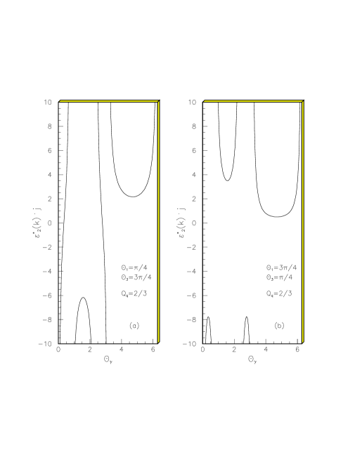
Figure 4: The radiation pattern of Eq. (25). Two (a) or no (b) radiation zeros are visible.

The generalisation to the case of arbitrary $W$ decays is straightforward. Thus for

$$W^{-} \to f_{1}(r_{1},Q_{1})+\bar{f}_{2}(r_{2},Q_{2}=1-Q_{1})$$

$$W^{+} \to f_{3}(r_{3},Q_{3})+\bar{f}_{4}(r_{4},Q_{4}=1-Q_{3})\;,$$ (27)

Eq. (25) becomes

$$-2Q_{q}\,\frac{1}{\sin\theta_{\gamma}}+Q_{1}\frac{\sin\theta_{1\gamma}}{1-\cos\theta_{1\gamma}}-(1-Q_{1})\frac{\sin\theta_{2\gamma}}{1+\cos\theta_{2\gamma}}$$

$$\hskip 42.67912pt-Q_{3}\frac{\sin\theta_{3\gamma}}{1-\cos\theta_{3\gamma}}+(1-Q_{3})\frac{\sin\theta_{4\gamma}}{1+\cos\theta_{4\gamma}}\,=\,0.$$ (28)

There are now either 4, 2 or 0 radiation zeros, depending on the relative orientation in the plane of the initial- and final-state particles.

(b) $\Gamma_{W}\ll E_{\gamma}\ll 1$

When the photon is far harder in energy than the $W$ is off mass shell (but still soft compared to the $W$ masses and energies), the timescale for photon emission is much shorter than the $W$ lifetime. As far as the photon is concerned, the overall process separates into ‘$W$ production’ and ‘$W$ decay’ pieces, with no interference between them. Formally, in this limit the profile functions are $\chi_{+-}=\chi_{-}=\chi_{+}=0$. Therefore all the interference terms in Eq. (3) vanish, and to find zeros one has to solve

$${\cal F}=|P|^{2}\,+\,|D^{+}|^{2}\,+\,|D^{-}|^{2}=0\;.$$ (29)

Since each of these quantities is positive definite they have to vanish separately:

$$|P|^{2} = 0\>\>\>{\rm RAZ\>\>of}\>\>q\bar{q}\,\to\,WW\gamma$$

$$|D^{+}|^{2} = 0\>\>\>{\rm RAZ\>\>of}\>\>W^{+}\,\to\,f_{3}\bar{f_{4}}\gamma$$

$$|D^{-}|^{2} = 0\>\>\>{\rm RAZ\>\>of}\>\>W^{-}\,\to\,f_{1}\bar{f_{2}}\gamma\quad.$$ (30)

Fortunately, the zeros of each are well-separated in phase space in regions that can be isolated experimentally. Thus in practice an energetic photon can be classified as a ‘production’ or a ‘decay’ photon depending on whether it reconstructs to an invariant mass $M_{W}$ when combined with the $W$ fermion decay products. Provided $E_{\gamma}\gg\Gamma_{W}$ this classification is in principle unambiguous. The radiation zeros for $W^{\pm}\to f\bar{f}\,^{\prime}\gamma$ decay have been known for some time, and in fact are directly analogous to those for $q\bar{q}\,^{\prime}\to W^{\pm}\gamma$ discussed in the previous section.

We therefore restrict our attention to the zeros of $q\bar{q}\to W^{+}W^{-}\gamma$, given by $|P|^{2}=0$, where the $W$s are now considered on-shell stable particles. It is straightforward to derive the expression for the current in this case (cf. Eq. (15)):

$$j^{\mu}\,=\,-\frac{k_{-}^{\mu}}{k_{-}\cdot k}+\,\frac{k_{+}^{\mu}}{k_{+}\cdot k}\,-Q_{q}\,\left(\frac{p_{1}^{\mu}}{p_{1}\cdot k}-\frac{p_{2}^{\mu}}{p_{2}\cdot k}\right)\;.$$ (31)

Then solving $\epsilon^{*}(k)\cdot j=0$ leads to

$$\tan\theta_{\gamma} = \frac{-\beta\,\sin\Theta-2\,Q_{q}\beta^{2}\cos\Theta\sin\Theta\pm\sqrt{\beta^{2}\,\sin^{2}\Theta+4\,Q_{q}(\beta^{2}-1)\,(Q_{q}+\beta\,\cos\Theta)}}{2\,(-\beta\,\cos\Theta-Q_{q}+Q_{q}\,\beta^{2}\,\sin^{2}\Theta)}$$

where $\beta=\left(1-M_{{W}}^{2}/E^{2}\right)^{\frac{1}{2}}<1$ is the velocity of the $W$, $\Theta$ is the angle between the $W^{-}$ and the incoming quark, and $E$ is the beam energy. Note that again these results correspond to all incoming and outgoing particles lying in the same plane. One interesting feature of this result is that there is now a certain minimum beam energy, for a given $\Theta$ and $Q_{q}$, which is required to set up the environment for radiation zeros (the square root in Eq. (3) has to be positive). For example, for $\Theta=\pi/2$ the critical energy is $E_{\mathrm{c}rit.}=M_{W}(1+4Q_{q}^{2})^{\frac{1}{2}}$. For energies $E>E_{\mathrm{c}rit.}$ four radiation zeros are present (due to the $\pm$ and the periodicity of $\tan$). For $E=E_{\mathrm{c}rit.}$ there are only two radiation zeros (the square root vanishes) and there are none for $E<E_{\mathrm{c}rit.}$. Note that for $\beta=1$ the $W$s can be regarded as massless particles and, as in the case (a) above, two zeros are present. But in practice $\beta<1$ and this gives rise to two additional zeros located close to the directions of the $W$s.

3.1 The general case

In the previous section we have found radiation zeros in the soft-photon approximation. In order to extend these results to arbitrary photon energies we have to consider the full matrix element, i.e. the sum of all the diagrams in Fig. 2. Since we are interested now in the case when $\Gamma_{W}\ll E_{\gamma}$, we can again make use of the partial fraction technique to factorise the full matrix element into production and decay parts, exactly as in Eqs. (29) and (3). As in the previous section we focus on the $WW\gamma$ production process:

$$d\,\sigma = \frac{1}{2s}d\,\Phi_{3}\,\,d\,\Phi_{2}^{+}\,\,d\,{\Phi_{2}^{-}}\,\,\big{|}\,\,{\cal M}_{1}+{\cal M}_{2}+{\cal M}_{3}+{\cal M}_{4}+{\cal M}_{9}\big{.}$$ (33)

$$\qquad\qquad+{\cal M}_{10}+{\cal M}_{11}+{\cal M}_{12}+{\cal M}_{13}+{\cal M}_{18}\,\,\big{|}^{2}$$

where the subscript refers to the diagrams of Fig. 2. The final-state fermion parts of these diagrams are integrated over the two-body phase spaces to give two branching ratio ($W\to f\bar{f}$) factors. The photon can be emitted off either the two initial-state quarks, the two final-state $W$’s, the internal lines ($W$’s as well as the $t-$channel quark) or from the four boson vertex.

We next have to specify the three-body phase space configuration. To simplify the kinematics we choose to fix the direction of the $W^{-}$ by $\Theta$, and the energy and the angle of the photon by $E_{\gamma}$ and $\theta_{\gamma}$ respectively. An overall azimuthal angle is disregarded and, more importantly, the incoming and outgoing particles are required to lie in a plane, defined by $\Phi=\phi_{\gamma}=0^{\circ}$. Given the initial quark momenta $p_{1},\,p_{2}$, the $W^{+}$ four-momentum is then constrained by energy-momentum conservation:

$$p_{1}^{\mu} = E(1,0,0,1)$$

$$p_{2}^{\mu} = E(1,0,0,-1)$$

$$k^{\mu} = E_{\gamma}(1,\sin\,\theta_{\gamma},0,\cos\,\theta_{\gamma})$$

$$k_{-}^{\mu} = (E_{W},\sqrt{E_{W}^{2}-M_{W}^{2}}\,\sin\,\Theta,0,\sqrt{E_{W}^{2}-M_{W}^{2}}\,\cos\,\Theta)$$

$$k_{+}^{\mu} = (2E-E_{\gamma}-E_{W},-(E_{\gamma}\sin\,\theta_{\gamma}+\sqrt{E_{W}^{2}-M_{W}^{2}}\,\sin\,\Theta),0,$$ (34)

$$\qquad\qquad\qquad-(E_{\gamma}\cos\,\theta_{\gamma}+\sqrt{E_{W}^{2}-M_{W}^{2}}\,\cos\,\Theta))$$

where $E_{W}$ is determined by the constraint $k_{+}^{2}=M_{W}^{2}$ and is given by

$$E_{W} = \left\{-2EE_{\gamma}^{2}-4E^{3}+6E^{2}E_{\gamma}+\left[E_{\gamma}^{2}\cos^{2}(\theta_{\gamma}-\Theta)\left(-8E^{3}E_{\gamma}+4E^{2}E_{\gamma}^{2}\right.\right.\right.$$ (35)

$$\left.\left.\left.\hskip 14.22636pt+M_{W}^{2}E_{\gamma}^{2}\cos^{2}(\theta_{\gamma}-\Theta)+4E^{4}-4E^{2}M_{W}^{2}+4EE_{\gamma}M_{W}^{2}-E_{\gamma}^{2}M_{W}^{2}\right)\right]^{\frac{1}{2}}\right\}$$

$$\hskip 28.45274pt/\left[E_{\gamma}^{2}\cos^{2}(\theta_{\gamma}-\Theta)-4E^{2}+4EE_{\gamma}-E_{\gamma}^{2}\right]\quad.$$

In terms of these variables the three-body phase space integration is

$$d\,\Phi_{3}(k_{+},k_{-},k)\,=\,\frac{E_{W}E_{\gamma}}{4(2\pi)^{5}}\,\frac{d\cos\Theta\,d\Phi\,\,dE_{\gamma}\,d\cos\theta_{\gamma}\,d\phi_{\gamma}\,}{\left|-4E+2E_{\gamma}-2E_{W}E_{\gamma}\cos(\theta_{\gamma}-\Theta)/\sqrt{E_{W}^{2}-M_{W}^{2}}\right|^{2}}\;.$$ (36)

We first consider the differential cross section as a function of $\theta_{\gamma}$, with all other variables kept fixed. For input parameters we take [8]

(39)

and in the following plots we also fix, for sake of illustration,

$$Q_{q}=\frac{2}{3}\;,\qquad E=500\;{\rm GeV}\;,\qquad\Theta=\frac{2\pi}{3}\;.$$ (40)

Fig. 5 shows the $\theta_{\gamma}$ dependence of the differential $u\bar{u}\to W^{+}W^{-}\gamma$ cross section, for a selection of photon energies $E_{\gamma}$. It is immediately apparent that an actual zero of the cross section is only achieved in the limit $E_{\gamma}\to 0$. Increasing the photon energy gradually ‘fills in’ the dip. The reason is that for non-soft photons additional diagrams (9 and 18 in Fig. 2) contribute and these give rise to a non-zero cross section at the positions of the zeros. The points at the bottom of the dips in Fig. 5 are actually the minimum values of the corresponding cross sections. In fact it can be shown that for $E_{\gamma}$ not too large, $\sigma_{\rm min}\propto E_{\gamma}$. At high photon energies the dips disappear altogether and the cross section assumes a different shape.

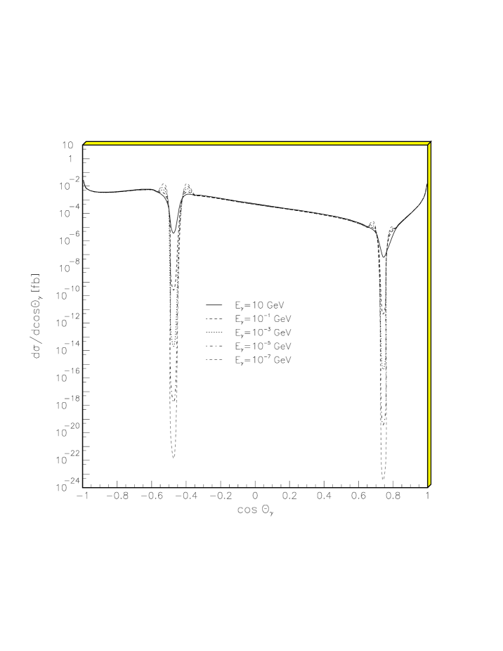
Figure 5: Differential cross section for the process $u\bar{u}\to W^{+}W^{-}\gamma$.

Note that the ‘zeros’/ dips both lie in the angular region between the outgoing $W^{-}$ and the incoming $u$, and by symmetry between the outgoing $W^{+}$ and the incoming $\bar{u}$. Further note that for a given $E_{\gamma}$, $\sigma_{\mathrm{m}in}$ differs by a factor $\sim 100$ due to the asymmetric (with respect to the photon emission angle) contribution from diagram 18.

To confirm that we do indeed have a Type II (planar configuration) radiation zero, we next recalculate the $\cos\theta_{\gamma}$ distribution for $\phi_{\gamma}\neq 0^{\circ}$. We choose a small non-zero photon energy $E_{\gamma}=10^{-5}$ GeV such that the dip is clearly visible for $\phi_{\gamma}=0^{\circ}$. The results are shown in Fig. 6. For $\phi_{\gamma}$ well away from zero, there is no hint of a dip in the cross section.

Figure 6: Same as Fig. 5 for $E_{\gamma}=10^{-5}$ GeV and various $\phi_{\gamma}$.

The results displayed in the above figures correspond to $u\,\bar{u}$ scattering. Similar results are obtained for $d\,\bar{d}$ and $e^{+}\,e^{-}$ scattering, i.e. exact Type II zeros are only found in the soft-photon limit where they are given by Eq. (3). The position of the zeros depends on the incoming fermions’ electric charge, and on the scattering angles and velocities of the $W$ bosons. For non-soft photons the dips are filled in, but still remain clearly visible for photon energies up to ${\cal O}(10\;{\rm GeV})$.

4 Anomalous gauge boson couplings

As discussed in the Introduction, the existence of radiation zeros is in general destroyed by the presence of anomalous gauge boson couplings. Two categories of such couplings are usually considered — trilinear and quartic gauge boson couplings — and each probes different aspects of the weak interactions. The trilinear couplings directly test the non-Abelian gauge structure, and possible deviations from the SM forms have been extensively studied in the literature, see for example [9] and references therein. Experimental bounds have also been obtained [10]. In contrast, the quartic couplings can be regarded as a more direct window on electroweak symmetry breaking, in particular to the scalar sector of the theory (see for example [11]) or, more generally, on new physics which couples to electroweak bosons. In this respect it is quite possible that the quartic couplings deviate from their SM values while the triple gauge vertices do not. For example, if the mechanism for electroweak symmetry breaking does not reveal itself through the discovery of new particles such as the Higgs boson, supersymmetric particles or technipions, it is possible that anomalous quartic couplings could provide the first evidence of new physics in this sector of the electroweak theory [11].

The impact of anomalous trilinear couplings on the radiation zeros in the $q\bar{q}^{\prime}\to W\gamma$ process was considered in Ref. [12]. As expected, the zeros are removed for non-zero values of the anomalous parameters. Such couplings would also affect the zeros in the $WW\gamma$ case. However there are already quite stringent limits on these trilinear couplings from the Tevatron $p\bar{p}\to W\gamma X$ [13] and LEP2 $e^{+}e^{-}\to W^{+}W^{-}$ processes [10]. We therefore neglect them here and concentrate on genuine anomalous quartic couplings, for which no limits exist at present. The $WW\gamma$ process is in fact the simplest one which is sensitive to quartic couplings. It is natural therefore to consider the implications of anomalous quartic couplings on the radiation zeros discussed in the previous section.

The lowest dimension operators which lead to genuine quartic couplings where at least one photon is involved are of dimension 6 [14]. First, we have the neutral and charged Lagrangians, both giving anomalous contributions to the $VV\gamma\gamma$ vertex, with $VV$ either being $W^{+}W^{-}$ or $Z^{0}Z^{0}$.

$${\cal L}_{0} = -\frac{e^{2}}{16\Lambda^{2}}\,a_{0}\,F^{\mu\nu}\,F_{\mu\nu}\stackrel{{\scriptstyle\longrightarrow}}{{W^{\alpha}}}\cdot\stackrel{{\scriptstyle\longrightarrow}}{{W_{\alpha}}}$$ (41)

$$= -\frac{e^{2}}{16\Lambda^{2}}\,a_{0}\,\big{[}-2(k_{1}\cdot k_{2})(A\cdot A)+2(k_{1}\cdot A)(k_{2}\cdot A)\big{]}$$

$$\hskip 42.67912pt{\times}\big{[}2(W^{+}\cdot W^{-})+(Z\cdot Z)/\cos^{2}\theta_{w}\big{]}\quad,$$

$${\cal L}_{c} = -\frac{e^{2}}{16\Lambda^{2}}\,a_{c}\,F^{\mu\alpha}\,F_{\mu\beta}\stackrel{{\scriptstyle\longrightarrow}}{{W^{\beta}}}\cdot\stackrel{{\scriptstyle\longrightarrow}}{{W_{\alpha}}}$$ (42)

$$= -\frac{e^{2}}{16\Lambda^{2}}\,a_{c}\,\big{[}-(k_{1}\cdot k_{2})\,A^{\alpha}A_{\beta}+(k_{1}\cdot A)\,A^{\alpha}k_{2\beta}\big{.}$$

$$\hskip 51.21504pt\big{.}\quad\quad+(k_{2}\cdot A)\,k_{1}^{\alpha}A_{\beta}-(A\cdot A)\,k_{1}^{\alpha}k_{2\beta}\big{]}$$

$$\hskip 42.67912pt{\times}\big{[}W_{\alpha}^{-}W^{+\beta}+W_{\alpha}^{+}W^{-\beta}+Z_{\alpha}Z^{\beta}/{\cos^{2}\theta_{w}}\big{]}\ .$$

where $k_{1}$ and $k_{2}$ are the photon momenta. Since we are interested in the anomalous $WW\gamma\gamma$ contribution we select the corresponding part of the Lagrangian.

Second, an anomalous $WWZ\gamma$ vertex is obtained from the Lagrangian

$${\cal L}_{n} = -\frac{e^{2}}{16\Lambda^{2}}\,a_{n}\epsilon_{ijk}W_{\mu\alpha}^{(i)}W_{\nu}^{(j)}W^{(k)\alpha}F^{\mu\nu}$$ (43)

$$= -\frac{e^{2}}{16\Lambda^{2}\cos\theta_{w}}\,a_{n}\,\big{(}k^{\nu}A^{\mu}-k^{\mu}A^{\nu}\big{)}$$

$${\times}\left(-W^{-}_{\nu}k_{\mu}^{+}\,(Z\cdot W^{+})+W_{\nu}^{+}k_{\mu}^{-}\,(Z\cdot W^{-})+Z_{\nu}k_{\mu}^{+}\,(W^{+}\cdot W^{-})\right.$$

$$-Z_{\nu}k_{\mu}^{-}\,(W^{+}\cdot W^{-})+W_{\nu}^{-}W_{\mu}^{+}\,(k^{+}\cdot Z)-W_{\nu}^{+}W_{\mu}^{-}\,(k^{-}\cdot Z)$$

$$-Z_{\nu}W_{\mu}^{+}\,(k^{+}\cdot W^{-})+Z_{\nu}W_{\mu}^{-}\,(k^{-}\cdot W^{+})-W^{+}_{\nu}k^{0}_{\mu}\,(Z\cdot W^{-})$$

$$\left.+W_{\nu}^{-}k^{0}_{\mu}\,(Z\cdot W^{+})-W_{\nu}^{-}Z_{\mu}\,(k^{0}\cdot W^{+})+W_{\nu}^{+}Z_{\mu}\,(k^{0}\cdot W^{-})\right)$$

where $k,k^{+},k^{-}$ and $k^{0}$ are the momenta of the photon, $W^{+}$, $W^{-}$ and $Z^{0}$ respectively.

Let us consider first the differential cross section in the planar configuration as a function of $\theta_{\gamma}$, just as we did in the previous section, but now in the presence of non-zero values of the three anomalous parameters $a_{0},\,a_{c}$ and $a_{n}$ introduced above. From the Lagrangian it can be seen that any anomalous contribution is linear in $E_{\gamma}$. Soft photons are ‘blind’ to the anomalous couplings and therefore the zeros in the $k^{\mu}\to 0$ limit survive. For moderate photon energies, the dips in the SM cross section will be filled in by contributions proportional to $a_{i}$ and $a_{i}^{\phantom{i}2}$. The higher the photon energy, the more dramatic the effect, although of course the dips become less well defined too. In principle, therefore, one should optimize the photon energy, to make it small enough to maintain the zeros but at the same time large enough to gain measurable deviations from the SM prediction. Since the anomalous contributions originate in the four boson vertex in the $s$-channel, one can also increase the sensitivity to them by considering only right-handed initial quarks, for which the $t$-channel contributions are absent.

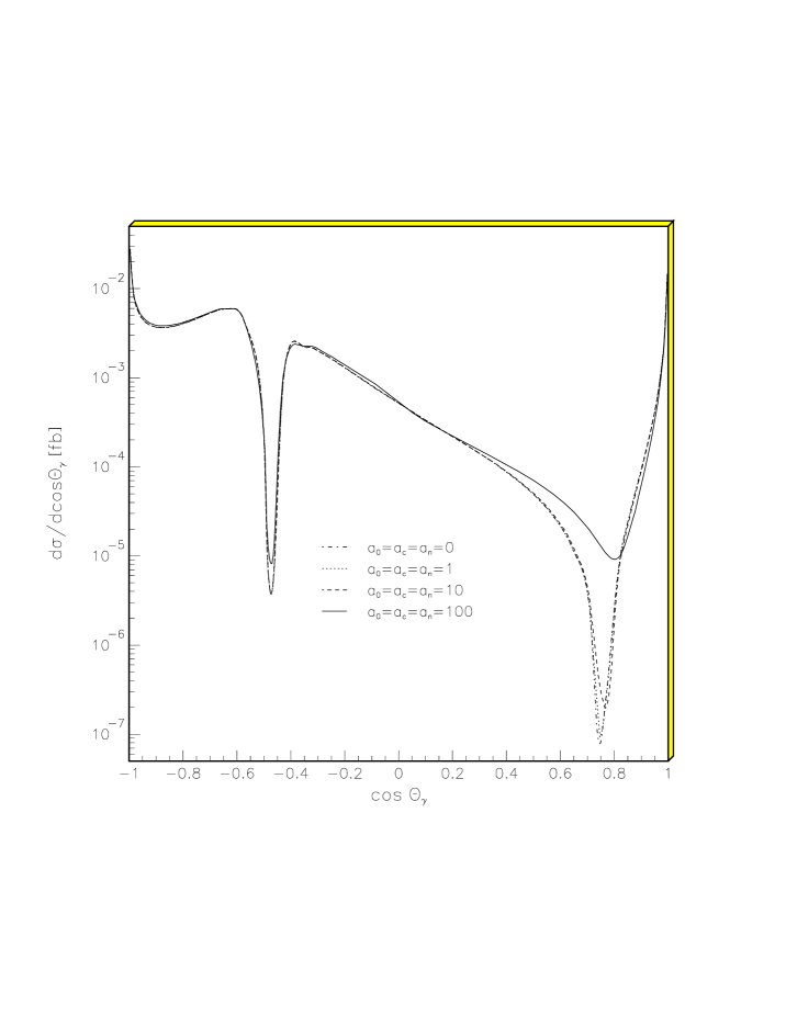
Figure 7: Differential cross section for the process $u\bar{u}\to W^{+}W^{-}\gamma$ with $E_{\gamma}=1$ GeV. The curves correspond to different values of the anomalous parameters introduced in the text.

Fig. 7 shows the $\theta_{\gamma}$ dependence of the $u\bar{u}\to WW\gamma$ cross section for $E_{\gamma}=1$ GeV, for the same configuration and parameters as in Fig. 5 (see Eqs. (39,40)). The curves correspond to different (positive) values of the anomalous parameters . The anomalous contribution is approximately isotropic in $\theta_{\gamma}$. Therefore because the dips have different depths one gets filled in more rapidly than the other. This is evident in the figure, where the dip at $\cos\theta_{\gamma}\sim 0.75$ is already filled in for $a_{i}\sim{\cal O}(100)$, whereas the steep dip at $\cos\theta_{\gamma}\sim-0.48$ is still very apparent. This shows it is advantageous to focus on certain regions of photon phase space in order to increase the sensitivity to the anomalous couplings. Of course, this requires very high luminosity to ensure a large enough event rate in these regions.

5 Conclusions

We have investigated the (Type II) radiation zeros of the process $q\bar{q}\to W^{+}W^{-}\gamma\to f_{1}\bar{f}_{2}f_{3}\bar{f}_{4}\gamma$. In the soft-photon limit ($\Gamma_{W}\ll E_{\gamma}\ll 1$) the cross section vanishes for certain values of the photon and $W^{\pm}$ production angles, for which analytic expressions have been derived (Eq. (3)). For non-zero photon energies the zeros disappear, but for energies not too large the photon angular distribution still exhibits deep dips centred on the positions of the soft-photon zeros. The subtle cancellations leading to the zeros in the soft-photon limit still takes place, but for non-soft photons two additional diagrams (9 and 18) have to be considered and $\sigma_{\mathrm{m}in}$ is exactly that contribution. In the ‘classic‘ process $q\bar{q}\,^{\prime}\to W^{+}\gamma$ there are no further diagrams for non-soft photons and the zeros survive for all photon energies. Although we have concentrated on the quark scattering process $q\bar{q}\to W^{+}W^{-}\gamma$ our results apply equally well to $e^{+}e^{-}\to W^{+}W^{-}\gamma$ by setting $Q_{q}=-1$. Note that, as for quark antiquark scattering, the zeros in the $e^{+}e^{-}$ (soft-photon) case are in the ‘visible’ regions of phase space, in contrast to those in the analogous ‘classical’ process $e^{+}\nu_{e}\to W^{+}\gamma$. Furthermore for $e^{+}e^{-}$ scattering diagram 9 (scattering via $t$-channel exchange) is not present and direct access to the four boson vertex is given for non-soft photons, i.e. the four boson vertex is the only contribution to the cross section at the position of the zeros.

We have also studied the effect of including non-zero anomalous quartic couplings. These contributions increase with increasing photon energy and fill in the dips present in the standard model. In principle, therefore, the vicinity of the radiation zeros is the most sensitive part of phase space to these anomalous four boson couplings.

Our analysis has been entirely theoretical. Having established that there are regions of phase space where the cross section is heavily suppressed, the next step is to see to what extent the phenomenon persists when hadronisation, radiative corrections, smearing, boost, detector etc. effects are taken into account, in the context, for example, of a possible measurement at the Tevatron or LHC hadron colliders. In this respect, a high energy, high luminosity $e^{+}e^{-}$ linear collider could provide a cleaner environment for studying $WW\gamma$ production in this way.

Acknowledgements
This work was supported in part by the EU Fourth Framework Programme ‘Training and Mobility of Researchers’, Network ‘Quantum Chromodynamics and the Deep Structure of Elementary Particles’, contract FMRX-CT98-0194 (DG 12 - MIHT). AW gratefully acknowledges financial support in the form of a ‘DAAD Doktorandenstipendium im Rahmen des gemeinsamen Hochschulprogramms III für Bund und Länder’.

References

[1] K.O. Mikaelian, M.A. Samuel and D. Sahdev, Phys. Rev. Lett.43 (1979) 746.
[2] R.W. Brown, Understanding Something about Nothing: Radiation Zeros,
published in Vector Boson Symp. 1995: 261-272.
R.W. Brown, K.L. Kowalski and S.J. Brodsky Phys. Rev.D28 (1983) 624.
[3] D. Benjamin for the CDF collaboration,
and production at the Tevatron, FERMILAB-Conf-95-241-E.
[4] R. Kleiss and W.J. Stirling, Nucl. Phys.B262 (1985) 235.
[7] M. Heyssler and W.J. Stirling, Eur. Phys. J.C4 (1998) 289.
[8] C. Caso et al., Review of Particle Physics, Eur. Phys. J.C3 (1998) 1.
[9] K. Hagiwara, R.D. Peccei, D. Zeppenfeld and K. Hikasa,
Nucl. Phys.B282 (1987) 253.
Triple Gauge Boson Couplings,
G. Gounaris et al.,
in ‘Physics at LEP2’, Vol. 1, p. 525-576, CERN (1995) [hep-ph/9601233].
[10] ALEPH Collaboration: R. Barate et al., Phys. Lett.B422 (1998) 369;
preprint CERN-EP-98-178, November 1998 [hep-ex/9901030].
OPAL Collaboration: G. Abbiendi et al., preprint CERN-EP-98-167,
October 1998 [hep-ex/9811028].
[11] S. Godfrey, Quartic Gauge Boson Couplings,
published in Proceedings of the International Symposium on Vector Boson Self-Interactions,
UCLA, Feb. 1-3, 1995.
[12] T. Abraha and M.A. Samuel, Oklahoma State U. preprint OSU–RN–326,
hep-ph/9706336.
[13]H.T. Diehl, Boson Pair Production and Triple Gauge Couplings, FERMILAB-CONF-97-216-E.
[14] G.Blanger and F. Boudjema, Phys. Lett.B288 (1992) 201.
[15] W.J. Stirling and A. Werthenbach, preprint hep-ph/9903315.