Hard-thermal-loop Resummation
of the Thermodynamics of a Hot Gluon Plasma

Abstract

We calculate the thermodynamic functions of a hot gluon plasma to leading order in hard-thermal-loop (HTL) perturbation theory. Effects associated with screening, gluon quasiparticles, and Landau damping are resummed to all orders. The ultraviolet divergences generated by the HTL propagator corrections can be canceled by a counterterm that depends on the thermal gluon mass parameter. The HTL thermodynamic functions are compared to those from lattice gauge theory calculations and from quasiparticle models. For reasonable values of the HTL parameters, the deviations from lattice results for $T>2T_{c}$ have the correct sign and roughly the correct magnitude to be accounted for by next-to-leading order corrections in HTL perturbation theory.

I Introduction

Relativistic heavy-ion collisions will soon allow the experimental study of hadronic matter at energy densities that will probably exceed that required to create a quark-gluon plasma. A quantitative understanding of the properties of a quark-gluon plasma is essential in order to determine whether it has been created. Because QCD, the gauge theory that describes strong interactions, is asymptotically free, its running coupling constant $\alpha_{s}$ becomes weak at sufficiently high temperatures. This would seem to make the task of understanding the high-temperature limit of hadronic matter relatively straightforward, because the problem can be attacked using perturbative methods. Unfortunately, a straightforward perturbative expansion in powers of $\alpha_{s}$ does not seem to be of any quantitative use even at temperatures that are orders of magnitude higher than those achievable in heavy-ion collisions.

The problem is evident in the free energy ${\cal F}$ of the quark-gluon plasma, whose weak-coupling expansion has been calculated through order $\alpha_{s}^{5/2}$ [1, 2, 3]. An optimist might hope to use perturbative methods at temperatures as low as 0.3 GeV, because the running coupling constant $\alpha_{s}(2\pi T)$ at the scale of the lowest Matsubara frequency is about 1/3. Unfortunately, the weak-coupling expansion seems to diverge badly even at much higher temperatures. For a pure-glue plasma, the first few terms in the weak-coupling expansion are

$${\cal F}_{\rm QCD} = {\cal F}_{\rm ideal}\Bigg{[}1\;-\;{15\over 4}{\alpha_{s}\over\pi}\;+\;30\left({\alpha_{s}\over\pi}\right)^{3/2}$$ (3)

$$\;+\;{135\over 2}\left(\log{\alpha_{s}\over\pi}-{11\over 36}\log{\mu_{4}\over 2\pi T}+3.51\right)\left({\alpha_{s}\over\pi}\right)^{2}$$

$$+{495\over 2}\left(\log{\mu_{4}\over 2\pi T}-3.23\right)\left({\alpha_{s}\over\pi}\right)^{5/2}\;+\;{\cal O}(\alpha_{s}^{3}\log\alpha_{s})\Bigg{]},$$

where ${\cal F}_{\rm ideal}=-(8\pi^{2}/45)T^{4}$ is the free energy of an ideal gas of massless gluons and $\alpha_{s}=\alpha_{s}(\mu_{4})$ is the running coupling constant in the $\overline{\mbox{MS}}$ scheme. In Fig. 1, the free energy is shown as a function of $T/T_{c}$, where $T_{c}$ is the critical temperature for the deconfinement transition. The weak-coupling expansions through orders $\alpha_{s}$, $\alpha_{s}^{3/2}$, $\alpha_{s}^{2}$, and $\alpha_{s}^{5/2}$ are shown as bands that correspond to varying the renormalization scale $\mu_{4}$ by a factor of two from the central value $\mu_{4}=2\pi T$. As successive terms in the weak-coupling expansion are added, the predictions fluctuate wildly and the sensitivity to the renormalization scale grows. Of course, because of asymptotic freedom, the first few terms in the weak-coupling expansion will appear to converge at sufficiently high temperature. However, this occurs only at temperatures orders of magnitude larger than $T_{c}$. For example, the $\alpha_{s}^{3/2}$ term is smaller than the $\alpha_{s}$ term only if $\alpha_{s}$ is less than about 1/20, which corresponds to a temperature greater than about $10^{5}T_{c}$. It is clear that a reorganization of the perturbative series is essential if perturbative calculations are to be of any quantitative use at temperatures accessible in heavy-ion collisions.

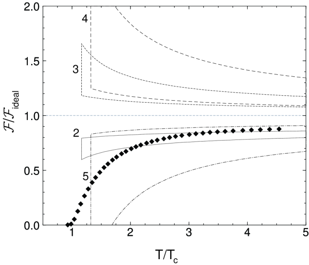
FIG. 1.: The free energy for pure-glue QCD as a function of $T/T_{c}$. The weak-coupling expansions through orders $\alpha_{s}$, $\alpha_{s}^{3/2}$, $\alpha_{s}^{2}$, and $\alpha_{s}^{5/2}$ are shown as bands that correspond to varying the renormalization scale $\mu_{4}$ by a factor of two. The lattice results from Boyd et al. [4] are shown as diamonds.

The poor convergence of the perturbative series is puzzling, because lattice gauge theory calculations indicate that the free energy ${\cal F}$ of the quark-gluon plasma can be approximated by that of an ideal gas unless the temperature $T$ is very close to $T_{c}$ [4, 5]. In Fig. 1, we also show the lattice results for the free energy of pure-glue QCD from Boyd et al. [4]. The free energy approaches that of an ideal gas of massless gluons from below as the temperature is increased and the deviation is less than about 25% if $T$ is greater than $2T_{c}$.

There are many possible ways to reorganize the perturbation series for the free energy in order to improve its convergence. One possibility is to apply Padé approximation methods to the expansion in $\alpha_{s}^{1/2}$ [6]. This does improve the convergence somewhat, but it is at best a recipe with little physical motivation. There are also technical problems associated with the fact that the weak-coupling expansion is not simply a power series in $\alpha_{s}^{1/2}$. Effective field theory methods can be used to show that it has the general form

$${\cal F}_{\rm QCD}=T^{4}\sum_{n=0}^{\infty}c_{n}(\log\alpha_{s})\alpha_{s}^{n/2},$$ (4)

where the coefficients $c_{n}(\log\alpha_{s})$ are polynomials in $\log\alpha_{s}$ [7]. The first few coefficients can be calculated using perturbative methods and are given in (3). Beginning at order $\alpha_{s}^{3}$, nonperturbative methods are required to calculate some of the coefficients. Another problem with the Padé approximation method is that it is applicable only if several terms in the perturbative series are known. This essentially limits its applicability to the free energy ${\cal F}$ and to the other thermodynamic functions that can be obtained from $\cal F$ by differentiation. Almost all calculations involving signatures of the quark-gluon plasma have been carried out only to leading order. The only exception is the production of hard dileptons which has been calculated to next-to-leading order in $\alpha_{s}$ [8].

Another approach to the problem is based on the observation that the large corrections of order $\alpha_{s}^{3/2}$ and $\alpha_{s}^{5/2}$ in (3) arise from the momentum scale $gT$. Effective field-theory methods can be used to separate the momentum scale $T$ from the lower scales $gT$ and $g^{2}T$. The resulting effective field theory, dimensionally-reduced QCD (DRQCD), is an $SU(3)$ gauge theory with adjoint scalars in three euclidean dimensions. The construction of DRQCD can be used to separate the free energy into contributions from the scale $T$ and from lower scales:

$${\cal F}(T) = {\cal F}_{0}(T,\alpha_{s})+Tf_{1}(m_{E}^{2},g_{E}^{2},...).$$ (5)

The function ${\cal F}_{0}$ and the parameters $m_{E}^{2}$, $g_{E}^{2}$, … of the effective field theory can be computed as power series in $\alpha_{s}(2\pi T)$ by matching the effective field theory with thermal QCD. For pure-glue QCD, the parameters of DRQCD at leading order in $\alpha_{s}$ are $m_{E}^{2}=g^{2}T^{2}$, $g_{E}^{2}=g^{2}T$. The function $f_{1}$ can be expanded in powers of $g_{E}^{2}/m_{E}$ and the coefficients of the first three terms are known analytically [3]. The first term gives the large $\alpha_{s}^{3/2}$ correction in (3). The third term contributes $-830(\alpha_{s}/\pi)^{5/2}$ to the expansion in (3) and therefore accounts for most of the large $\alpha_{s}^{5/2}$ correction. Thus the poor convergence properties of the QCD perturbative series seems to arise from a breakdown of perturbation theory in DRQCD. This suggests that nonperturbative methods should be used to compute the second term in (5) as a function of the parameters $m_{E}^{2}$, $g_{E}^{2}$, … of DRQCD. The only systematic nonperturbative method currently available is Monte Carlo simulations of lattice DRQCD. This method has been developed by Kajantie, Rummukainen, and Shaposhnikov [9], and used to compute the Debye screening mass for thermal QCD [10]. It has not yet been applied to the free energy. One disadvantage of this method is that it relies in an essential way on the analytic continuation of the quantum field theory to imaginary time. It therefore cannot be used to calculate signatures of the quark-gluon plasma that involve real-time processes.

The poor convergence of the weak-coupling expansion for the free energy is not specific to QCD. The free energy of a massless scalar field theory with a $\phi^{4}$ interaction has also been computed to order $g^{5}$ [11]. The series seems to converge only if the coupling constant $g$ is extremely small. The largest corrections, which include the $g^{3/2}$ term, come from the momentum scale $gT$. This suggests that the source of the convergence problem could be similar for QCD and the massless scalar theory.

There have been several other attempts to improve the convergence of the free energy for the massless scalar field theory [12, 13]. One of the most successful approaches is “screened perturbation theory” developed by Karsch, Patkós, and Petreczky[12]. This approach can be made more systematic by using the framework of “optimized perturbation theory”, which has been applied by Chiku and Hatsuda to a scalar field theory with spontaneous symmetry breaking [14]. A local mass term proportional to $\phi^{2}$ is added and subtracted from the lagrangian, with the added term included nonperturbatively and the subtracted term treated as a perturbation. The renormalizability of the $\phi^{2}$ term guarantees that all ultraviolet divergences generated by the mass term can be systematically removed by renormalization. When the free energy is calculated using screened perturbation theory, the convergence of successive approximations to the free energy is dramatically improved.

Conventional perturbation theory is essentially an expansion about an ideal gas of massless particles. Screened perturbation theory is a reorganization of perturbation theory such that the expansion is about an ideal gas of quasiparticles with a temperature-dependent mass. Empirical evidence that such a reorganization of perturbation theory might be useful for QCD is provided by the success of quasiparticle models for the thermodynamics of QCD at temperatures above $T_{c}$. There were several early attempts to fit the thermodynamic functions calculated by lattice gauge theory to those of an ideal gas of massive quarks and gluons [16, 17]. In recent years, there have been several significant improvements in the lattice gauge theory calculations. The thermodynamic functions for pure-glue QCD have been calculated with very high precision by Boyd et al. [4]. There have also been calculations with $N_{f}=2$ and 4 flavors of dynamical quarks [5]. Motivated by these developments, more quantitative comparisons with quasiparticle models have been carried out by Peshier et al. [18] and by Lévai and Heinz [19]. These analyses indicate that the lattice results can be fit surprisingly well by an ideal gas of massive quarks and gluons with temperature-dependent masses $m_{q}(T)$ and $m_{g}(T)$ that grow approximately linearly with $T$.

A straightforward application of screened perturbation theory to gauge theories like QCD would be doomed to failure, because a local mass term for gluons is not gauge invariant. There is a way to incorporate plasma effects, including quasiparticle masses, screening of the gauge interaction and Landau damping, into perturbative calculations while maintaining gauge invariance and that is by using hard-thermal-loop (HTL) perturbation theory. Hard-thermal-loop perturbation theory was originally developed to sum up all higher loop corrections that are leading order in $g$ for amplitudes having soft external lines with momenta of order $gT$ [20]. If it is applied to amplitudes with hard external lines with momenta of order $T$, it selectively resums corrections that are higher order in $g$. This resummation is a generalization of screened perturbation theory that respects gauge invariance. It corresponds essentially to expanding around an ideal gas of quark and gluon quasiparticles.

HTL perturbation theory is defined by adding and subtracting hard-thermal-loop correction terms to the action [20]. The HTL correction terms are nonlocal, and the resulting effective propagators and vertices are complicated functions of the energies and momenta. Calculations in HTL perturbation theory are therefore much more difficult than in screened perturbation theory. The nonlocality of the HTL correction terms also introduces conceptual problems associated with renormalization. Since these terms are not renormalizable in the standard sense, the general structure of the ultraviolet divergences that they generate is not known.

If HTL perturbation theory proves to be tractable and if issues associated with renormalization can be resolved, it could have very important applications. It is a reorganization of QCD perturbation theory around a starting point that is essentially an ideal gas of massive quasiparticles. In contrast to quasiparticle models, the corrections due to interactions between quasiparticles can be calculated systematically, at least through next-to-next-to-leading order in HTL perturbation theory. Beyond that order perturbative calculations must be supplemented by a nonperturbative method to deal with the magnetic mass problem. A significant advantage of HTL perturbation theory over the approach using lattice gauge theory calculations in DRQCD is that it can be readily applied to the real-time processes that are the most promising signatures of a quark-gluon plasma.

In this paper, we calculate the free energy of a hot gluon plasma explicitly to leading order in hard-thermal-loop perturbation theory. In spite of the complexity of the HTL propagators, their analytic properties can be used to make explicit calculations possible. Although complicated ultraviolet divergences arise in the calculation, the most severe divergences cancel between quasiparticle and Landau-damping contributions and between transverse and longitudinal contributions. The remaining divergences arise from integrating over large three-momentum and can be removed by a counterterm proportional to $m_{g}^{4}$ at the expense of introducing a renormalization scale. With reasonable choices of the renormalization scales, our leading order result for the HTL free energy lies below results from lattice QCD for $T>2T_{c}$. However, the deviation from lattice QCD results has the correct sign and roughly the correct magnitude to be accounted for by next-to-leading order corrections in HTL perturbation theory.

II HTL Resummation

We begin this section by defining screened perturbation theory for a scalar field theory. We then define hard-thermal-loop perturbation theory, which is a generalization of screened perturbation theory that respects gauge invariance. Finally, we write down a formal expression for the free energy at leading order in HTL perturbation theory.

A Screened Perturbation Theory

The lagrangian density for a massless scalar field with a $\phi^{4}$ interaction is

$${\cal L}={1\over 2}\partial_{\mu}\phi\partial^{\mu}\phi-{1\over 24}g^{2}\phi^{4}+\Delta{\cal L}(g^{2}),$$ (6)

where $g$ is the coupling constant and $\Delta{\cal L}$ includes counterterms. The conventional perturbative expansion in powers of $g^{2}$ generates ultraviolet divergences, and the counterterm $\Delta{\cal L}$ must be adjusted to cancel the divergences order by order in $g^{2}$. At nonzero temperature, the conventional perturbative expansion also generates infrared divergences. They can be removed by resumming the higher order diagrams that generate a thermal mass of order $gT$ for the scalar particle. This resummation changes the perturbative series from an expansion in powers of $g^{2}$ to an expansion in powers of $\left(g^{2}\right)^{1/2}=g$. Unfortunately, the perturbative expansion for the free energy has large coefficients and appears to be convergent only for tiny values of $g$[11].

Screened perturbation theory, which was introduced by Karsch, Patkós and Petreczky [12], is simply a reorganization of the perturbation series for thermal field theory. It can be made more systematic by using a framework called “optimized perturbation theory” that Chiku and Hatsuda [14] have applied to a spontaneously broken scalar field theory. The Lagrangian density is written as

$${\cal L}={\cal L}-{1\over 2}(m^{2}-\delta m^{2})\phi^{2}+\Delta{\cal L}_{\rm s}(g^{2},m^{2}-\delta m^{2}),$$ (7)

where $\delta=1$ will be used as a formal expansion parameter and $\Delta{\cal L}_{\rm s}$ includes the additional counterterms that are required to remove ultraviolet divergences for $\delta\neq 1$. If we simply set $\delta=1$, the additional terms in (7) vanish. Screened perturbation theory is defined by taking $m^{2}$ to be of order $g^{0}$ and $\delta$ to be of order $g^{2}$, expanding systematically in powers of $g$ and setting $\delta=1$ at the end of the calculation. This defines a reorganization of perturbation theory in which the expansion is around the free field theory defined by

$${\cal L}_{\rm free}={1\over 2}\partial_{\mu}\phi\partial^{\mu}\phi-{1\over 2}m^{2}\phi^{2}.$$ (8)

The effects of the $m^{2}$ term in (8) are included to all orders, but they are systematically subtracted out at higher orders in perturbation theory by the $\delta m^{2}$ term in (7).

This reorganization of perturbation theory generates new ultraviolet divergences, but they can be canceled by the additional counterterms in $\Delta{\cal L}_{\rm s}$. The renormalizability of the lagrangian in (7) guarantees that the only counterterms that are required are $\partial_{\mu}\phi\partial^{\mu}\phi$, $\phi^{2}$, and $\phi^{4}$. At nonzero temperature, screened perturbation theory does not generate any infrared divergences, because the mass parameter $m^{2}$ in the free lagrangian (8) provides an infrared cutoff. The resulting perturbative expansion is therefore a power series in $g^{2}$ whose coefficients depend on the mass parameter $m^{2}$.

The parameter $m^{2}$ in screened perturbation theory is completely arbitrary. To complete a calculation in screened perturbation theory, it is necessary to specify $m^{2}$ as a function of $g^{2}$ and $T$. Karsch, Patkós, and Petreczky used the solution of a gap equation as their prescription for $m^{2}(T)$. The resulting loop expansion for the free energy appeared to be convergent.

In the weak coupling limit $g\to 0$, the solution to the gap equation for $m^{2}(T)$ approaches $g^{2}T^{2}/24$. If we use this value for $m^{2}$ and then reexpand the perturbative series for the free energy in powers of $g$, we recover the conventional perturbative expansion in powers of $g$, with its lack of convergence. It is therefore essential to keep the full dependence of $m^{2}$ at every order in $g^{2}$ and not expand in powers of $m/T$.

B HTL Perturbation Theory

Renormalized perturbation theory for pure-glue QCD can be defined by expressing the QCD lagrangian density in the form

$${\cal L}_{\rm QCD}=-{1\over 2}{\rm Tr}\left(G_{\mu\nu}G^{\mu\nu}\right)+{\cal L}_{\rm gf}+{\cal L}_{\rm ghost}+\Delta{\cal L}_{\rm QCD},$$ (9)

where $G_{\mu\nu}=\partial_{\mu}A_{\nu}-\partial_{\nu}A_{\mu}-ig[A_{\mu},A_{\nu}]$ is the gluon field strength and $A_{\mu}$ is the gluon field expressed as a matrix in the $SU(3)$ algebra. The ghost term ${\cal L}_{\rm ghost}$ depends on the choice of the gauge-fixing term ${\cal L}_{\rm gf}$. The perturbative expansion in powers of $g$ generates ultraviolet divergences, and the counterterms in $\Delta{\cal L}_{\rm QCD}$ are adjusted to cancel those divergences order by order in $g$.

Hard-thermal-loop (HTL) perturbation theory is simply a reorganization of the perturbation series for thermal QCD. The lagrangian density is written as

$${\cal L}_{\rm QCD}={\cal L}_{\rm QCD}+{\cal L}_{\rm HTL}+\Delta{\cal L}_{\rm HTL}(g,m_{g}^{2}-\delta m_{g}^{2}).$$ (10)

The HTL improvement term is

$${\cal L}_{\rm HTL}=-{3\over 2}(m_{g}^{2}-\delta m_{g}^{2}){\rm Tr}\left(G_{\mu\alpha}\left\langle{n^{\alpha}n^{\beta}\over(n\cdot D)^{2}}\right\rangle_{\!\!n}G^{\mu}_{\;\;\beta}\right),$$ (11)

where $D_{\mu}$ is the covariant derivative in the adjoint representation, $n^{\mu}=(1,\hat{{\bf n}})$ is a light-like four-vector, $\langle\ldots\rangle_{n}$ represents the average over the directions of $\hat{{\bf n}}$, and $\delta=1$ is a formal expansion parameter. The term (11) is the effective lagrangian that would be induced by a rotationally invariant ensemble of colored sources with infinitely high momentum. The parameter $m_{g}$ can be identified with the plasma frequency, or equivalently, with the rest mass of a gluon quasiparticle.

If we set $\delta=1$, the coefficient of the HTL improvement term (11) vanishes. HTL perturbation theory is defined by taking $m_{g}^{2}$ to be of order $g^{0}$ and $\delta$ to be formally of order $g^{2}$, expanding systematically in powers of $g$, and then setting $\delta=1$ at the end of the calculation. This defines a reorganization of the perturbative series in which some of the effects of the $m_{g}^{2}$ term in (11) are included to all orders but then systematically subtracted out at higher orders in perturbation theory by the $\delta m^{2}_{g}$ term. If the perturbative corrections from the $\delta m_{g}^{2}$ term could be summed to all orders, there would be no dependence on $m_{g}$. However, any truncation of the expansion in $\delta$ produces results that depend on $m_{g}$.

The term $\Delta{\cal L}_{\rm HTL}$ in (11) includes the counterterms required to cancel the new ultraviolet divergences generated by the reorganization of the perturbative series. Unlike the counterterms $\Delta{\cal L}_{\rm QCD}$ in (10) which are constrained by locality and renormalizability, the general structure of the terms in $\Delta{\cal L}_{\rm HTL}$ is unknown. We anticipate that if we use a scale-invariant regularization method such as dimensional regularization, the terms in $\Delta{\cal L}_{\rm HTL}$ will be polynomials in the parameters $g$ and $m_{g}^{2}-\delta m_{g}^{2}$.

The free lagrangian that serves as a starting point for HTL perturbation theory is obtained by setting $g=0$ and $\delta=0$ in (10). Choosing a covariant gauge-fixing term with gauge parameter $\xi$, the free lagrangian is

$${\cal L}_{\rm free} = -{\rm Tr}\left(\partial_{\mu}A_{\nu}\partial^{\mu}A^{\nu}-\partial_{\mu}A_{\nu}\partial^{\nu}A^{\mu}\right)-{1\over\xi}{\rm Tr}\left(\left(\partial^{\mu}A_{\mu}\right)^{2}\right)$$ (13)

$$-{3\over 2}m_{g}^{2}\mbox{Tr}\left((\partial_{\mu}A_{\alpha}-\partial_{\alpha}A_{\mu})\left\langle{n^{\alpha}n^{\beta}\over(n\cdot\partial)^{2}}\right\rangle_{\!\!n}(\partial^{\mu}A_{\beta}-\partial_{\beta}A^{\mu})\right).$$

The HTL improvement term generates a self-energy tensor for the gluon that is diagonal in the color indices and has the form

$$\Pi^{\mu\nu}(K)=-{3\over 2}m_{g}^{2}\left\langle{K^{2}n^{\mu}n^{\nu}-n\cdot K(K^{\mu}n^{\nu}+n^{\mu}K^{\nu})+(n\cdot K)^{2}g^{\mu\nu}\over(K\cdot n)^{2}}\right\rangle_{\!\!n},$$ (14)

where $K^{\mu}=(k_{0},{\bf k})$ is the Minkowski four-momentum and $K^{2}=k_{0}^{2}-{\bf k}^{2}$. The HTL self-energy tensor satisfies the Ward identity $K_{\mu}\Pi^{\mu\nu}=0$. Because of this Ward identity and the rotational symmetry around the axis $\hat{{\bf k}}$, the tensor $\Pi^{\mu\nu}$ can be expressed in terms of two independent functions $\Pi_{L}$ and $\Pi_{T}$:

$$\Pi^{\mu\nu}(K)=-\Pi_{L}(K){K^{2}g^{\mu\nu}-K^{\mu}K^{\nu}\over k^{2}}+\left[\Pi_{T}(K)-{K^{2}\over k^{2}}\Pi_{L}(K)\right]g^{\mu i}(\delta^{ij}-\hat{k}^{i}\hat{k}^{j})g^{j\nu}.$$ (15)

The longitudinal and transverse self-energies are

$$\Pi_{L}(K) = \Pi^{00}(K),$$ (16)

$$\Pi_{T}(K) = ={1\over 2}\left(\delta^{ij}-\hat{k}^{i}\hat{k}^{j}\right)\Pi^{ij}(K).$$ (17)

The inverse propagator for the gluon is diagonal in the color indices and has the form

$$\Delta^{-1}(K)^{\mu\nu} = -K^{2}g^{\mu\nu}+\left(1-{1\over\xi}\right)K^{\mu}K^{\nu}+\Pi^{\mu\nu}(K).$$ (18)

If there are $d$ spatial dimensions, the matrix $\Delta^{-1}(K)^{\mu}_{\;\;\nu}$ has $d+1$ eigenvalues: $-K^{2}(k^{2}-\Pi_{L})/k^{2}$, $-K^{2}/\xi$, and the $(d-1)$-fold degenerate eigenvalue $K^{2}-\Pi_{T}$. The inverse propagator for the ghost in a general covariant gauge is $\Delta^{-1}_{\rm ghost}=K^{2}$.

In the general Coulomb gauge, the gauge-fixing term in (13) is replaced by $-(1/\xi){\rm Tr}\left(\left(\nabla\cdot{\bf A}\right)^{2}\right)$. The term $-(1/\xi)K^{\mu}K^{\nu}$ in the inverse gluon propagator (18) is replaced by $-(1/\xi)g^{\mu i}k^{i}k^{j}g^{j\nu}$. The $d+1$ eigenvalues of $\Delta^{-1}(K)^{\mu}_{\;\;\nu}$ are the $(d-1)$-fold degenerate eigenvalue $K^{2}-\Pi_{T}$ and two other eigenvalues whose product is $-k^{2}(k^{2}-\Pi_{L})/\xi$. The inverse propagator for the ghost in this gauge is $k^{2}$. The limit $\xi\rightarrow 0$ is the strict Coulomb gauge defined by the constraint $\nabla\cdot{\bf A}=0$. In this gauge, the only propagating modes of the gluon are $A_{0}$ and the $d-1$ transverse components of ${\bf A}$. The propagators are $k^{2}-\Pi_{L}$ for $A_{0}$ and $K^{2}-\Pi_{T}$ for the transverse components of ${\bf A}$.

C HTL Free Energy

In the imaginary-time formalism, the renormalized one-loop free energy can be written as

$${\cal F}_{\rm HTL}=(N_{c}^{2}-1)\left[{1\over 2}\hbox{$\sum$}\!\!\!\!\!\!\int_{K}{\rm Tr}\log\Delta^{-1}(K)-\hbox{$\sum$}\!\!\!\!\!\!\int_{K}\log\Delta_{\rm ghost}^{-1}(K)+\Delta{\cal F}\right],$$ (19)

where $\Delta^{-1}$ and ${\Delta}^{-1}_{\rm ghost}$ are the euclidean inverse propagators for gluons and ghosts, and $K$ is now a euclidean four-momentum: $K^{\mu}=(\omega_{n},{\bf k})$, and $K^{2}=k^{2}+\omega^{2}_{n}$. The sum-integral in (19) represents a dimensionally regularized integral over the momentum ${\bf k}$ and a sum over the Matsubara frequencies $\omega_{n}=2\pi nT$:

$$\hbox{$\sum$}\!\!\!\!\!\!\int_{K}\equiv T\sum_{n=-\infty}^{\infty}\mu^{3-d}\int{d^{d}k\over(2\pi)^{d}}.$$ (20)

The factor of $\mu^{3-d}$, where $\mu$ is a renormalization scale, ensures that the regularized free energy has correct dimensions even for $d\neq 3$. The counterterm $\Delta{\cal F}$ in (19) can be used to cancel ultraviolet divergences that have the form of an additive constant in the free energy.

In the gluon term in (19), the integrand is the sum of the logarithms of the $d+1$ eigenvalues of $\Delta^{-1}$. After taking into account the cancellations from the ghost term and dropping terms that vanish in dimensional regularization, the expression (19) for the HTL free energy reduces to

$${\cal F}_{\rm HTL}\;=\;(N_{c}^{2}-1)\left[(d-1){\cal F}_{T}+{\cal F}_{L}\;+\;\Delta{\cal F}\right],$$ (21)

where

$${\cal F}_{T} = {1\over 2}\hbox{$\sum$}\!\!\!\!\!\!\int_{K}\log[K^{2}+\Pi_{T}(K)],$$ (22)

$${\cal F}_{L} = {1\over 2}\hbox{$\sum$}\!\!\!\!\!\!\int_{K}\log[k^{2}-\Pi_{L}(K)].$$ (23)

An identical expression for the free energy is obtained in the general Coulomb gauge. The free energies ${\cal F}_{T}$ and ${\cal F}_{L}$ have simple interpretations in the strict Coulomb gauge. They are simply the contributions to the free energy from a transverse component of ${\bf A}$ and from $A_{0}$, respectively. We therefore refer to them as the transverse and longitudinal free energies.

At first sight, the calculation of the HTL free energy appears to be a rather daunting mathematical problem. The HTL self-energy functions in (22) and (23) are

$$\Pi_{T}(\omega_{n},k) = -{3\over 2}m_{g}^{2}{\omega_{n}^{2}\over k^{2}}\left[1+{\omega^{2}_{n}+k^{2}\over 2i\omega_{n}k}\log{i\omega_{n}+k\over i\omega_{n}-k}\right],$$ (24)

$$\Pi_{L}(\omega_{n},k) = 3m_{g}^{2}\left[{i\omega_{n}\over 2k}\log{i\omega_{n}+k\over i\omega_{n}-k}-1\right].$$ (25)

In order to calculate the HTL free energy, we must evaluate the sum-integrals in (22) and (23) with a regularization that cuts off the ultraviolet divergences. In the next section, we show that this problem can be made tractable by using the analytic properties of the HTL self-energies.

III HTL Free Energy

In this section, we reduce the HTL free energy to integrals that can be evaluated numerically. We first compute the free energy of a free massless boson as a simple example. We then compute the transverse and longitudinal free energies, separating them into quasiparticle and Landau-damping terms and isolating the ultraviolet divergences into integrals that can be computed analytically. The most severe divergences cancel, leaving a logarithmic divergence that must be canceled explicitly by a counterterm.

A Free Massless Boson

As a warm-up exercise for computing the transverse free energy, we compute the free energy of a free massless boson:

$${\cal F}_{\rm boson}={1\over 2}\hbox{$\sum$}\!\!\!\!\!\!\int_{K}\log(K^{2}).$$ (26)

In dimensional regularization, the $n=0$ term in the sum-integral vanishes. For the same reason, we can subtract $\log k^{2}$ from the integrand for each of the $n\neq 0$ terms. The free energy becomes

$${\cal F}_{\rm boson}={1\over 2}T\sum_{n\neq 0}\int_{\bf k}\log{k^{2}+\omega_{n}^{2}\over k^{2}}.$$ (27)

We have introduced a compact notation for the dimensionally regularized integral over momentum together with the renormalization scale factor:

$$\int_{\bf k}\equiv\mu^{3-d}\int{d^{d}k\over(2\pi)^{d}}.$$ (28)

The sum over Matsubara frequencies in (27) can be expressed as a contour integral:

$${\cal F}_{\rm boson}={1\over 2}\int_{C}{d\omega\over 2\pi i}\int_{\bf k}\log{k^{2}-\omega^{2}\over k^{2}}{1\over e^{\beta\omega}-1},$$ (29)

where the contour $C$ encloses the points $\omega=i\omega_{n}$, $n\neq 0$, as shown in Fig. 2.

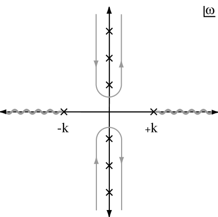
FIG. 2.: The free energy of a massless boson can be expressed as an integral over a contour $C$ that can be deformed into two contours that wrap around the branch cuts of $\log(k^{2}-\omega^{2})$.

We can choose the branch cuts of the logarithm to run along the real $\omega$-axis from $-\infty$ to $-k$ and from $+k$ to $+\infty$. It is convenient to insert a convergence factor $e^{\eta\omega}$ ($\eta\rightarrow 0^{+}$) into the integrand. This allows the contour $C$ in Fig. 2 to be deformed into two contours that wrap around the branch cuts. Collapsing the contour onto the two branch cuts, making the change of variables $\omega\to-\omega$ in the contribution from the negative branch cut, and taking the limit $\eta\rightarrow 0$ whenever it is not needed for convergence, the free energy reduces to

$${\cal F}_{\rm boson}=-\int_{\bf k}\int_{k}^{\infty}d\omega\left({1\over e^{\beta\omega}-1}+{1\over 2}e^{-\eta\omega}\right).$$ (30)

Integrating over $\omega$ and taking the limit $\eta\rightarrow 0$, we obtain

$${\cal F}_{\rm boson}=\int_{\bf k}\left[T\log(1-e^{-\beta k})-{1\over 2\eta}+{1\over 2}k\right].$$ (31)

The integral over the last two terms are zero in dimensional regularization. Setting $d=3$ in the integral of the first term in (31) and evaluating it analytically, we get

$${\cal F}_{\rm boson}=-{\pi^{2}\over 90}T^{4}.$$ (32)

Summing over the $N_{c}^{2}-1$ color degrees of freedom and the two spin degrees of freedom of a transverse gluon, we obtain the free energy of an ideal gas of massless gluons:

$${\cal F}_{\rm ideal}=-\left(N_{c}^{2}-1\right){\pi^{2}\over 45}T^{4}.$$ (33)

B Transverse Free Energy

We now proceed to compute the transverse free energy in (22). Following the steps that led from (26) to (29), we obtain the contour integral

$${\cal F}_{T}={1\over 2}\int_{C}{d\omega\over 2\pi i}\int_{\bf k}\log{k^{2}-\omega^{2}+\Pi_{T}(-i\omega,k)\over k^{2}}{e^{\eta\omega}\over e^{\beta\omega}-1},$$ (34)

where $e^{\eta\omega}$ ($\eta\rightarrow 0^{+}$) is a convergence factor and the contour $C$ encloses the points $\omega=i\omega_{n},n\neq 0$. The integrand has logarithmic branch cuts in $\omega$ that run along the real $\omega$-axis from $-\infty$ to $-\omega_{T}(k)$ and from $+\omega_{T}(k)$ to $+\infty$, where $\omega_{T}(k)$ is the quasiparticle dispersion relation for transverse gluons. This dispersion relation satisfies $k^{2}-\omega_{T}^{2}+\Pi_{T}(-i\omega_{T},k)=0$, or

$$\omega_{T}^{2} = k^{2}\;+\;{3\over 2}m_{g}^{2}{\omega_{T}^{2}\over k^{2}}\left[1-{\omega_{T}^{2}-k^{2}\over 2\omega_{T}k}\log{\omega_{T}+k\over\omega_{T}-k}\right].$$ (35)

The integrand also has a branch cut in $\omega$ running from $-k$ to $+k$ due to the function $\Pi_{T}$. This branch cut represents the effects of Landau damping. The contour $C$ can be deformed into a contour that wraps around the three branch cuts as in Fig. 3.

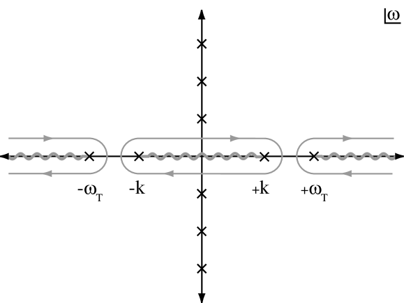
FIG. 3.: The transverse free energy can be expressed as an integral over a contour $C$ that wraps around three branch cuts of $\log(k^{2}-\omega^{2}+\Pi_{T})$.

We identify the contribution from the branch cuts ending at $\pm\omega_{T}(k)$ as the quasiparticle part of ${\cal F}_{T}$ and denote it by ${\cal F}_{T,{\rm qp}}$. Following the same steps that led to (31), we obtain

$${\cal F}_{T,{\rm qp}}=\int_{\bf k}\left[T\log(1-e^{-\beta\omega_{T}})+{1\over 2}\omega_{T}\right].$$ (36)

We have omitted the term $1/(2\eta)$ in the integrand of (36) because its integral vanishes in dimensional regularization. We identify the contribution from the contour wrapping around the branch cut running from $-k$ to $+k$ as the Landau-damping part of ${\cal F}_{T}$ and denote it by ${\cal F}_{T,{\rm Ld}}$. Collapsing the contour onto the branch cut and expressing it as an integral over positive values of $\omega$, we obtain

$${\cal F}_{T,{\rm Ld}}=-{1\over\pi}\int_{\bf k}\int_{0}^{k}d\omega\;\phi_{T}\left[{1\over e^{\beta\omega}-1}+{1\over 2}\right].$$ (37)

The angle $\phi_{T}$ is

$$\phi_{T}(\omega,k)=\arctan{{3\pi\over 4}m^{2}_{g}{\omega K^{2}\over k^{3}}\over K^{2}\;+\;{3\over 2}m^{2}_{g}{\omega^{2}\over k^{2}}\left[1+{K^{2}\over 2k\omega}L\right]},$$ (38)

where $K^{2}=k^{2}-\omega^{2}$ and $L=\log\left[{(k+\omega)/(k-\omega)}\right]$. The angle $\phi_{T}(\omega,k)$ vanishes as $\omega\rightarrow 0$ and as $k\rightarrow\infty$ and it also vanishes at $\omega=k$. The complete transverse energy ${\cal F}_{T}$ is the sum of the quasiparticle term (36) and the Landau-damping term (37). The integral of the second term in (36) and the integral of both terms in (37) are ultraviolet divergent, but the divergences are regularized by the $d$-dimensional integral over ${\bf k}$. In order to extract the divergences analytically, we make subtractions in the integrands that render the integrals finite in $d=3$ dimensions and then extract the poles in $d-3$ from the subtracted integrals.

We first consider the transverse quasiparticle term (36). The integral of the second term is divergent, because the asymptotic form of the transverse dispersion relation for large $k$ is [22]

$$\omega_{T}(k)\longrightarrow k+{3\over 4}{m_{g}^{2}\over k}-{9\over 32}{m_{g}^{4}\over k^{3}}\left(2\log{8k^{2}\over 3m_{g}^{2}}-3\right).$$ (39)

Our subtraction should make the integral ultraviolet convergent for $d=3$, and it should not introduce any infrared divergences. Our choice for the subtracted integral is

$${\cal F}_{T,{\rm qp}}^{(\rm sub)}={1\over 2}\int_{\bf k}\left[\sqrt{k^{2}+\mbox{${3\over 2}$}m_{g}^{2}}-{9m_{g}^{4}\over 16(k^{2}+{3\over 2}m^{2}_{g})^{3/2}}\left(\log{8(k^{2}+{3\over 2}m_{g}^{2})\over 3m_{g}^{2}}-2\right)\right].$$ (40)

After subtracting this from (36), we can take the limit $d\rightarrow 3$:

$${\cal F}_{T,{\rm qp}}-{\cal F}_{T,{\rm qp}}^{(\rm sub)} = {T\over 2\pi^{2}}\int^{\infty}_{0}k^{2}dk\log(1-e^{-\beta\omega_{T}})$$ (42)

$$+{1\over 4\pi^{2}}\int^{\infty}_{0}k^{2}dk\left[\omega_{T}-\sqrt{k^{2}+\mbox{${3\over 2}$}m_{g}^{2}}+{9m_{g}^{4}\over 16(k^{2}+{3\over 2}m^{2}_{g})^{3/2}}\left(\log{8(k^{2}+{3\over 2}m_{g}^{2})\over 3m_{g}^{2}}-2\right)\right].$$

If we impose a momentum cutoff $k<\Lambda$, our subtraction integral (40) has power divergences proportional to $\Lambda^{4}$ and $m_{g}^{2}\Lambda^{2}$ and logarithmic divergences proportional to $m_{g}^{4}\log\Lambda$ and $m_{g}^{4}\log^{2}\Lambda$. The quartic divergence is canceled by the usual renormalization of the vacuum energy density at zero temperature. Dimensional regularization throws away the power divergences and replaces the logarithmic divergences by poles in $d-3$. In the limit $d\rightarrow 3$, the individual integrals in (40) are given by (A.1)–(A.3) in the appendix. The result is

$${\cal F}_{T,\rm qp}^{\rm(sub)}=-{9\over 64}m_{g}^{4}\left(3m_{g}^{2}\over 2\mu^{2}\right)^{-\epsilon}{\Omega_{d}\over(2\pi)^{d}}\left[{1\over\epsilon^{2}}+{4\log 2-3\over 2}{1\over\epsilon}+2\log^{2}2-3\log 2+{\pi^{2}\over 6}-{1\over 4}\right],$$ (43)

where $\epsilon=(3-d)/2$ and $\Omega_{d}=2\pi^{d/2}/\Gamma(d/2)$ is the angular integral in $d$ dimensions.

We next consider the Landau-damping term (37). Again we must choose a subtraction term that removes the ultraviolet divergences without introducing infrared divergences. Our choice is

$${\cal F}_{T,\rm Ld}^{(\rm sub)} = -{1\over\pi}\int_{\bf k}\int_{0}^{k}d\omega\left[{3\pi m_{g}^{2}\omega\over 4k^{3}}{1\over e^{\beta\omega}-1}+{3\pi m_{g}^{2}\omega K^{2}\over 8k^{3}(K^{2}+{3\over 2}m_{g}^{2})}\right.$$ (45)

$$\left.\hskip 99.58464pt-{9\pi m_{g}^{4}\omega(K^{2})^{2}\over 16k^{5}(K^{2}+{3\over 2}m_{g}^{2})^{2}}\left({\omega\over 2k}L-1\right)\right].$$

After subtracting this from (37), we can take the limit $d\rightarrow 3$:

$${\cal F}_{T,{\rm Ld}}-{\cal F}_{T,{\rm Ld}}^{(\rm sub)} = -{1\over 2\pi^{3}}\int^{\infty}_{0}d\omega{1\over e^{\beta\omega}-1}\int^{\infty}_{\omega}k^{2}dk\left[\phi_{T}-{3\pi m_{g}^{2}\omega\over 4k^{3}}\right]$$ (47)

$$-{1\over 4\pi^{3}}\int^{\infty}_{0}d\omega\int^{\infty}_{\omega}k^{2}dk\Bigg{[}\phi_{T}-{3\pi m_{g}^{2}\omega K^{2}\over 4k^{3}(K^{2}+{3\over 2}m_{g}^{2})}+{9\pi m_{g}^{4}\omega(K^{2})^{2}\over 8k^{5}(K^{2}+{3\over 2}m_{g}^{2})^{2}}\left({\omega\over 2k}L-1\right)\Bigg{]}.$$

In both integrals, the first subtraction makes them convergent as $k\rightarrow\infty$ with $\omega$ fixed. The second subtraction in the second integral makes it convergent as $k\rightarrow\infty$ with $\omega\sim k$. If we impose ultraviolet cutoffs $\omega<\Lambda$ and $k<\Lambda$ on the energy and momentum, the subtraction integral (45) has a power divergence proportional to $m_{g}^{2}\Lambda^{2}$ and logarithmic divergences proportional to $m_{g}^{2}T^{2}\log\Lambda$, $m_{g}^{4}\log\Lambda$, and $m_{g}^{4}\log^{2}\Lambda$. The divergence proportional to $m_{g}^{4}\log^{2}\Lambda$ cancels against the corresponding divergence in the quasiparticle subtraction integral (40). The cancellation can be traced to the fact that $\Pi_{T}(\omega,k)$ is analytic in the variable $\omega$ at $\omega=\infty$. Dimensional regularization replaces the logarithmic divergences in (45) by poles in $d-3$ and sets the power divergences to zero. The integrals in (45) are evaluated in the limit $d\rightarrow 3$ in the appendix and given by (A.4)–(A.7) and (A.10). The result is

$${\cal F}_{T,\rm Ld}^{(\rm sub)} = -{\pi^{2}\over 16}m_{g}^{2}T^{2}\left({T^{2}\over\mu^{2}}\right)^{-\epsilon}{\Omega_{d}\over(2\pi)^{d}}\left[{1\over\epsilon}+2{\zeta^{\prime}(-1)\over\zeta(-1)}-2\log(2\pi)\right]$$ (49)

$$+{9\over 64}m_{g}^{4}\left({3m_{g}^{2}\over 2\mu^{2}}\right)^{-\epsilon}{\Omega_{d}\over(2\pi)^{d}}\left[{1\over\epsilon^{2}}+{2(\log 2-1)\over 3}{1\over\epsilon}+{2\over 3}\log^{2}2-{22\over 9}\log 2+{\pi^{2}\over 6}+{10\over 9}\right].$$

Our final result for the transverse self-energy is the sum of (42), (43), (47) and (49). Note that the divergence proportional to ${1/\epsilon^{2}}$ cancels between (43) and (49).

C Longitudinal Free Energy

We now compute the longitudinal free energy given in (23). We first separate out the $n=0$ term:

$${\cal F}_{L}={1\over 2}T\int_{\bf k}\log\left({k^{2}+3m^{2}_{g}}\right)+{1\over 2}T\sum_{n\neq 0}\int_{\bf k}\log\left({k^{2}-\Pi_{L}(\omega_{n},k)}\right).$$ (50)

These two terms can be expressed as a single integral over a contour $C$ that encloses the points $\omega=i\omega_{n},n\neq 0$:

$${\cal F}_{L}={1\over 2}\int_{C}{d\omega\over 2\pi i}\int_{\bf k}\log{k^{2}-\Pi_{L}(-i\omega,k)\over k^{2}+3m_{g}^{2}}{e^{\eta\omega}\over e^{\beta\omega}-1},$$ (51)

where $e^{\eta\omega}$ ($\eta\rightarrow 0^{+}$) is a convergence factor. The logarithm in the integrand can be expressed as the difference of two logarithms. The integral of the first logarithm reproduces the sum of the $n\neq 0$ terms in (50). In the contour integral of the $\log(k^{2}+3m_{g}^{2})$ term, the contour can be deformed to wrap around the pole at $\omega=0$ of the Bose-Einstein factor. By the residue theorem, this reproduces the $n=0$ term in (50).

The integrand in (51) has a logarithmic branch cut in $\omega$ that runs from $-\omega_{L}(k)$ to $+\omega_{L}(k)$, where $\omega_{L}(k)$ is the quasiparticle dispersion relation for longitudinal gluons. This dispersion relation satisfies $k^{2}-\Pi_{L}(-i\omega_{L},k)=0$ or

$$0 = k^{2}\;+\;3m_{g}^{2}\left[1-{\omega_{L}\over 2k}\log{\omega_{L}+k\over\omega_{L}-k}\right].$$ (52)

The integral also has a branch cut in $\omega$ running from $-k$ to $+k$ due to the function $\Pi_{L}$. This branch cut represents the effects of Landau damping. We choose both branch cuts to run along the real axis so that they overlap in the region $-k<\omega<k$.

The contour $C$ can be deformed into a contour that wraps around the branch cuts from as in Fig. 4, and the contour can then be collapsed onto the branch cut.

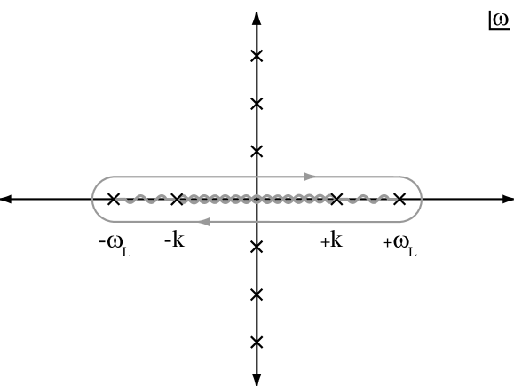
FIG. 4.: The longitudinal free energy can be expressed as an integral around a contour $C$ that wraps around the branch cuts of $\log(k^{2}-\Pi_{L})$.

We identify the contributions from $k<|\omega|<\omega_{L}(k)$ as the quasiparticle part of ${\cal F}_{L}$ and denote it by ${\cal F}_{L,\rm qp}$:

$${\cal F}_{L,\rm qp}=\int_{\bf k}\left[T\log{1-e^{-\beta\omega_{L}}\over 1-e^{-\beta k}}+{1\over 2}\left(\omega_{L}-k\right)\right].$$ (53)

We identify the contribution from $|\omega|<k$ as the Landau-damping part of ${\cal F}_{L}$ and denote it by ${\cal F}_{L,\rm Ld}$:

$${\cal F}_{L,\rm Ld}={1\over\pi}\int_{\bf k}\int_{0}^{k}d\omega\;\phi_{L}\left[{1\over e^{\beta\omega}-1}+{1\over 2}\right].$$ (54)

The angle $\phi_{L}$ is

$$\phi_{L}(\omega,k)=\arctan{{3\pi\over 2}m_{g}^{2}{\omega\over k}\over k^{2}\;+\;3m_{g}^{2}\left[1-{\omega\over 2k}L\right]},$$ (55)

where $L=\log\left[(k+\omega)/(k-\omega)\right]$. The angle $\phi_{L}(\omega,k)$ vanishes as $\omega\rightarrow 0$ and as $k\rightarrow\infty$ and its value is $\pi$ at $\omega=k$. The denominator of the argument of the arctangent in (55) vanishes at some point $\omega=\omega^{*}(k)$. The arctangent in (55) is the principal branch for $0<\omega<\omega^{*}(k)$, and it jumps to the next branch for $\omega^{*}(k)<\omega<k$, so that $\phi_{L}$ remains continuous.

The complete longitudinal free energy ${\cal F}_{L}$ is the sum of the quasiparticle term (53) and the Landau-damping term (54). The quasiparticle integral is convergent, because $\omega_{L}$ approaches $k$ as a gaussian at large $k$. The Landau-damping term has ultraviolet divergences that are regularized by the $d$-dimensional integral over $\bf k$. In order to extract the divergences analytically, we make subtractions in the integrand that make the integral convergent in $d=3$, and we then extract the poles in $d-3$ from the subtracted integral. Our choice of the subtracted integral is

$${\cal F}_{L,\rm Ld}^{(\rm sub)} = {1\over\pi}\int_{\bf k}\int_{0}^{k}d\omega\left[{3\pi m_{g}^{2}\omega\over 2k^{3}}{1\over e^{\beta\omega}-1}+{3\pi m_{g}^{2}\omega\over 4k(k^{2}+3m_{g}^{2})}\right.\left.+{9\pi m_{g}^{4}\omega^{2}\over 8k^{2}(k^{2}+3m_{g}^{2})^{2}}L\right].$$ (56)

After subtracting this from (54), we can take the limit $d\rightarrow 3$:

$${\cal F}_{L,{\rm Ld}}-{\cal F}_{L,\rm Ld}^{(\rm sub)} = {1\over 2\pi^{3}}\int^{\infty}_{0}d\omega{1\over e^{\beta\omega}-1}\int^{\infty}_{\omega}k^{2}dk\left[\phi_{L}-{3\pi m_{g}^{2}\omega\over 2k^{3}}\right]$$ (57)

$$+ {1\over 4\pi^{3}}\int^{\infty}_{0}d\omega\int^{\infty}_{\omega}k^{2}dk\left[\phi_{L}-{3\pi m_{g}^{2}\omega\over 2k(k^{2}+3m_{g}^{2})}-{9\pi m_{g}^{4}\omega^{2}\over 4k^{2}(k^{2}+3m_{g}^{2})^{2}}L\right].$$ (58)

If we impose ultraviolet cutoffs $\omega<\Lambda$ and $k<\Lambda$ on the energy and momentum, the subtraction integral (56) has a power divergence proportional to $m^{2}_{g}\Lambda^{2}$ and logarithmic divergences proportional to $m_{g}^{2}T^{2}\log\Lambda$ and $m_{g}^{4}\log\Lambda$. The divergence proportional to $m_{g}^{2}\Lambda^{2}$ cancels against the corresponding divergence in the transverse Landau-damping subtraction integral (45). Dimensional regularization throws away the quadratic divergence and replaces the logarithmic divergences by poles in $\epsilon$. In the limit $d\rightarrow 3$, the individual integrals in (56) are given by (A.8)–(A.10) in the appendix. The result is

$${\cal F}_{L,\rm Ld}^{(\rm sub)} = {\pi^{2}\over 8}m_{g}^{2}T^{2}\left({T^{2}\over\mu^{2}}\right)^{-\epsilon}{\Omega_{d}\over(2\pi)^{d}}\left[{1\over\epsilon}+2{\zeta^{\prime}(-1)\over\zeta(-1)}-2\log(2\pi)\right]$$ (60)

$$+{3\over 8}m_{g}^{4}\left({3m_{g}^{2}\over\mu^{2}}\right)^{-\epsilon}{\Omega_{d}\over(2\pi)^{d}}\left[{\log 2-1\over\epsilon}-\log 2-{1\over 2}\right].$$

Our final result for the longitudinal free energy is the sum of (53), (58) and (60).

D Renormalized Free Energy

To complete our calculation of the HTL free energy, we must determine the counterterm $\Delta{\cal F}$ in (21) that cancels the divergences in $(d-1){\cal F}_{T}+{\cal F}_{L}$. The ultraviolet divergences have been isolated in the subtraction terms (43) and (49) for ${\cal F}_{T}$ and (60) for ${\cal F}_{L}$. The poles in $\epsilon$ proportional to $m_{g}^{2}T^{2}$ cancel between ${\cal F}_{T}$ and ${\cal F}_{L}$. The cancellation can be traced to the fact that the logarithms cancels in the following combination of self-energy functions:

$$2{\Pi_{T}(-i\omega,k)\over\omega^{2}-k^{2}}+{\Pi_{L}(-i\omega,k)\over k^{2}}={3m_{g}^{2}\over\omega^{2}-k^{2}}.$$ (61)

The remaining divergence is proportional to $m_{g}^{4}$. In the minimal subtraction renormalization prescription, $\Delta{\cal F}$ is chosen to cancel only the pole in $\epsilon$ and no additional finite terms:

$$\Delta{\cal F}={9\over 128\pi^{2}\epsilon}m_{g}^{4}.$$ (62)

If we use a momentum cutoff $\Lambda$, there is also a quadratic divergence proportional to $m_{g}^{2}\Lambda^{2}$ coming from the transverse quasiparticle subtraction term (40). This would be canceled by an additional counterterm in (62) proportional to $m_{g}^{2}\Lambda^{2}$.

To obtain the final result for the HTL free energy, we insert into (21) the sum of (42), (43), (47) and (49) for ${\cal F}_{T}$, the sum of (53), (58) and (60) for ${\cal F}_{L}$, and (62) for $\Delta{\cal F}$. We can simplify the result by evaluating the temperature independent integrals numerically. Since the only scale in these integrals is the mass $m_{g}$, they reduce to $m_{g}^{4}$ multiplied by a numerical coefficient. The contributions to ${\cal F}_{T}$ from the second integral in (42) and the second integral in (47) are $-8.656\times 10^{-3}m_{g}^{4}$ and $-4.554\times 10^{-4}m_{g}^{4}$, respectively. The contribution to ${\cal F}_{L}$ from the integral of the second term in (53) and from the second integral in (58) are $1.225\times 10^{-2}m_{g}^{4}$ and $4.290\times 10^{-3}m_{g}^{4}$, respectively. Our final result for the renormalized free energy is

$${\cal F}_{\rm HTL} = \left(N_{c}^{2}-1\right)\Bigg{\{}{1\over 2\pi^{2}}T\int_{0}^{\infty}k^{2}dk\left[2\log(1-e^{-\beta\omega_{T}})+\log{1-e^{-\beta\omega_{L}}\over 1-e^{-\beta k}}\right]$$ (65)

$$\hskip 51.21504pt+{1\over 2\pi^{3}}\int_{0}^{\infty}d\omega\;{1\over e^{\beta\omega}-1}\int_{\omega}^{\infty}k^{2}dk\left[\phi_{L}-2\phi_{T}\right]$$

$$\hskip 51.21504pt+{1\over 16}m_{g}^{2}T^{2}+{9\over 64\pi^{2}}m_{g}^{4}\left[\log{m_{g}\over\mu_{3}}-0.332837\right]\Bigg{\}},$$

where $\mu_{3}=\sqrt{4\pi}e^{-\gamma}\mu$ is the renormalization scale associated with the modified minimal subtraction ($\overline{\mbox{MS}}$) renormalization prescription and $\gamma$ is Euler’s constant. The dispersion relations $\omega_{T}(k)$ and $\omega_{L}(k)$ are the solutions to (35) and (52). The angles $\phi_{T}(\omega,k)$ and $\phi_{L}(\omega,k)$ satisfy (38) and (55).

IV High-Temperature Expansion

If the temperature is much greater than the gluon mass parameter $m_{g}$, the HTL free energy can be expanded in powers of $m_{g}/T$. Such an expansion is contrary to the spirit of HTL perturbation theory, which is an expansion in powers of $g$ and $\delta$ with $m_{g}^{2}$ fixed. It is nevertheless interesting, because it can be compared directly with the perturbative expansion for the QCD free energy. In this section, we compute the high-temperature expansion for the HTL free energy through order $(m_{g}/T)^{4}$.

A Separation of Scales

The high-temperature expansion for the HTL free energy could be deduced directly from the final expression (65). However, this is difficult because of the delicate cancellations between quasiparticle and Landau-damping terms and between transverse and longitudinal contributions. It is easier to carry out the high-temperature expansion starting from dimensionally regularized contour integral expressions for ${\cal F}_{T}$ and ${\cal F}_{L}$. If we separate out the free energy of a massless boson given in (29), the transverse free energy (34) becomes

$${\cal F}_{T} = -{\pi^{2}\over 90}T^{4}+{1\over 2}\int_{C}{d\omega\over 2\pi i}\int_{\bf k}\log\left(1-{\Pi_{T}(-i\omega,k)\over\omega^{2}-k^{2}}\right){1\over e^{\beta\omega}-1}.$$ (66)

Since the logarithm goes to zero as $\omega\rightarrow\infty$, there is no need for a convergence factor $e^{\eta\omega}$. We can choose the logarithmic branch cut in (66) to run from $-\omega_{T}(k)$ to $-k$ and from $+k$ to $+\omega_{T}(k)$. The contour $C$ can then be deformed so that it wraps around the branch cuts that run along the real axis between $-\omega_{T}(k)$ and $+\omega_{T}(k)$. In the expression (50) for the longitudinal free energy, the first term can be evaluated analytically using (A.11). In the second term, it is convenient to subtract $\log k^{2}$ from the integrand before writing it as a contour integral as in (51). The resulting expression is

$${\cal F}_{L} = -{\sqrt{3}\over 4\pi}m_{g}^{3}T+{1\over 2}\int_{\bf k}\int_{C}{d\omega\over 2\pi i}\log\left(1-{\Pi_{L}(-i\omega,k)\over k^{2}}\right){1\over e^{\beta\omega}-1},$$ (67)

where the contour $C$ wraps around the branch cuts that run along the real axis between $-\omega_{L}(k)$ and $+\omega_{L}(k)$.

The integrals in (66) and (67) involve two energy and momentum scales: the “hard” scale $T$ and the “soft” scale $m_{g}$. The terms in the high-temperature expansion can receive contributions from both the hard scale and the soft scale. Dimensional regularization makes it easy to separate these contributions. We can obtain the soft contribution by expanding the Bose-Einstein factor in powers of $\omega/T$:

$${1\over e^{\beta\omega}-1}=\sum_{n=0}^{\infty}{B_{n}\over n!}\left({\omega\over T}\right)^{n-1}\,,$$ (68)

where $B_{n}$ are the Bernoulli numbers. The only scale in the resulting dimensionally regularized integral is $m_{g}$. Thus, upon inserting (68) into (66) and (67) , we obtain expansions in powers of $m_{g}/T$. These are the soft contributions to the high-temperature expansion. We can obtain the hard contributions by expanding the logarithms in (66) and (67) in powers of $m_{g}^{2}$ or, equivalently, in powers of $\Pi_{T}$ and $\Pi_{L}$:

$$\log\left(1-{\Pi_{T}(-i\omega,k)\over\omega^{2}-k^{2}}\right) = -\sum_{n=1}^{\infty}{1\over n}\left[{\Pi_{T}(-i\omega,k)\over\omega^{2}-k^{2}}\right]^{n},$$ (69)

$$\log\left(1-{\Pi_{L}(-i\omega,k)\over k^{2}}\right) = -\sum_{n=1}^{\infty}{1\over n}\left[{\Pi_{L}(-i\omega,k)\over k^{2}}\right]^{n}.$$ (70)

The resulting dimensionally regularized integrals involve only the scale $T$. Thus, upon inserting (69) and (70) into (66) and (67), we obtain expansions in powers of $m_{g}^{2}/T^{2}$. These are the hard contributions to the high-temperature expansion. In the next subsections, we calculate the expansions for the soft and the hard contributions through order $(m_{g}/T)^{4}$.

B Soft Contributions to ${\cal F}_{T}$ and ${\cal F}_{L}$

The soft contributions to the high-temperature expansion of the free energy consist of the first term in (67) and the soft contributions from the second terms in (66) and (67). We first consider the soft contribution to the transverse free energy. After inserting the expansion (68) into (66), there are no longer any poles on the imaginary $\omega$ axis. Having chosen the branch cuts to lie on the real axis in the interval $-\omega_{T}<\omega<\omega_{T}$, the contour $C$ can be taken to infinity in all directions. Making the change of variables $z=1/\omega$, the contour becomes a counterclockwise circle around $z=0$. The soft contribution to ${\cal F}_{T}$ can then be written as

$$-{1\over 2}\sum_{n=0}^{\infty}{B_{n}\over n!}T^{1-n}\int_{\bf k}\oint{dz\over 2\pi i}z^{-n-1}\log\left(1-{\Pi_{T}(-i/z,k)\over(1/z)^{2}-k^{2}}\right)\,.$$ (71)

The logarithmic factor is an even function of $z$ that is analytic at $z=0$. It can therefore be expanded as a power series in $z^{2}$:

$$\log\left(1-{\Pi_{T}(-i/z,k)\over(1/z)^{2}-k^{2}}\right)=\sum_{p=1}^{\infty}T_{p}(m,k)z^{2p}\,,$$ (72)

where $T_{p}(m,k)$ is a polynomial of degree $p$ in $m^{2}$ and $k^{2}$. Inserting this expansion into (71), the contour integral vanishes unless $n=2p$. The soft contribution (71) then reduces to

$$-{1\over 2}\sum_{p=1}^{\infty}{B_{2p}\over(2p)!}T^{1-2p}\int_{\bf k}T_{p}(m,k)\,.$$ (73)

However, since the integrand $T_{p}(m,k)$ is a polynomial in $k,$ the dimensionally regularized integral over ${\bf k}$ vanishes. The soft contribution to ${\cal F}_{T}$ is therefore zero.

We next consider the soft contributions to the longitudinal free energy coming from the second term in (67). Performing the change of variables $z=1/\omega$ yields

$$-{1\over 2}\sum_{n=0}^{\infty}{B_{n}\over n!}T^{1-n}\int_{\bf k}\oint{dz\over 2\pi i}z^{-n-1}\log\left(1-{\Pi_{L}(-i/z,k)\over k^{2}}\right),$$ (74)

where the contour is a counterclockwise circle around $z=0$. The logarithmic factor is an even function of $z$ that it is analytic at $z=0$. It therefore can be expanded as a power series in $z^{2}$:

$$\log\left(1-{\Pi_{L}(-i/z,k)\over k^{2}}\right)=\sum_{p=1}^{\infty}L_{p}(m,k)z^{2p}\,,$$ (75)

where $L_{p}(m,k)$ is a polynomial of degree $p$ in $m^{2}$ and $k^{2}$. The contour integral in (74) vanishes unless $n=2p$. But then the integral over ${\bf k}$ vanishes in dimensional regularization because $L_{p}$ is a polynomial in $k$. Thus the soft contribution to the second term of (67) is zero. The only contribution to the free energy from the soft momentum scale $m_{g}$ is therefore the first term in (67), which comes from the $n=0$ Matsubara mode.

C Hard Contribution to ${\cal F}_{T}$

The hard contributions to the high-temperature expansion of ${\cal F}_{T}$ consist of the $T^{4}$ term in (66) and the power series in $m_{g}^{2}$ obtained by inserting (69) into (66). The first term in that expansion is

$${\cal F}_{T}^{(1)}=-{1\over 2}\int_{\bf k}\int_{C}{d\omega\over 2\pi i}{\Pi_{T}(-i\omega,k)\over\omega^{2}-k^{2}}{1\over e^{\beta\omega}-1}.$$ (76)

The function multiplying the Bose-Einstein factor can be written as

$${\Pi_{T}(-i\omega,k)\over\omega^{2}-k^{2}}={3m_{g}^{2}\over 2k^{2}}\left({\omega^{2}\over\omega^{2}-k^{2}}-{\omega\over 2k}\log{\omega+k\over\omega-k}\right).$$ (77)

Thus the integrand in (76) is the sum of two terms, one with poles at $\omega=\pm k$ and the other with a branch cut that runs from $\omega=-k$ to $\omega=k$. The integral of the pole terms can be evaluated using the residue theorem. In the branch cut term, the contour can be collapsed onto the branch cut, and then expressed as an integral over positive values of $\omega$. The resulting expression is

$${\cal F}_{T}^{(1)} = {3\over 4}m_{g}^{2}\int_{\bf k}\left[{1\over k}\left({1\over e^{\beta k}-1}+{1\over 2}\right)-{1\over k^{3}}\int_{0}^{k}d\omega\;\omega\left({1\over e^{\beta\omega}-1}+{1\over 2}\right)\right].$$ (78)

The integrals can be evaluated analytically. In the last term, the integrand is evaluated by integrating first over $k$ and then over $\omega$. The final result is

$${\cal F}_{T}^{(1)} = -{\pi^{2}\over 16}m^{2}_{g}T^{2}\left({T^{2}\over\mu^{2}}\right)^{-\epsilon}{\Omega_{d}\over(2\pi)^{d}}\left[{1\over\epsilon}+2\log{\zeta^{\prime}(-1)\over\zeta(-1)}-2\log(2\pi)-2\right].$$ (79)

The second term in the expansion of ${\cal F}_{T}$ in powers of $m_{g}^{2}$ is

$${\cal F}_{T}^{(2)}=-{1\over 4}\int_{\bf k}\int_{C}{d\omega\over 2\pi i}\left({\Pi_{T}(-i\omega,k)\over\omega^{2}-k^{2}}\right)^{2}{1\over e^{\beta\omega}-1}.$$ (80)

Using (77), we can separate the integrand from (80) into a double pole term, a double logarithm term, and terms that are products of a single pole and a logarithm. After using the residue theorem and collapsing the contour onto the branch cut, the expression (80) reduces to

$${\cal F}_{T}^{(2)} = {9\over 32}m_{g}^{4}\int_{\bf k}\left\{{3+2\epsilon\over k^{3}}\left({1\over e^{\beta k}-1}+{1\over 2}\right)\right.+{2\over k^{6}}\int_{0}^{k}d\omega\;\omega^{3}{\partial\over\partial\omega}\left({1\over e^{\beta\omega}-1}\right)\log{k+\omega\over k-\omega}$$ (82)

$$\left.-{8\over k^{6}}\int_{0}^{k}d\omega\;\omega^{2}\log{k+\omega\over k-\omega}\left({1\over e^{\beta\omega}-1}+{1\over 2}\right)\right\}.$$

The double integrals can be evaluated by integrating first over $k$ and then over $\omega$. Expanding around $\epsilon=0$ and keeping terms only through order $\epsilon^{0}$, the final result is

$${\cal F}_{T}^{(2)} = -{3\over 16}m_{g}^{4}\left({T^{2}\over\mu^{2}}\right)^{-\epsilon}{\Omega_{d}\over(2\pi)^{d}}\left[{8\log 2-5\over 8}\left({1\over\epsilon}-2\log(2\pi)+2\gamma+{1\over 3}\right)-{7\over 8}+{\pi^{2}\over 12}\right.\Bigg{]}.$$ (83)

D Hard contribution to ${\cal F}_{L}$

The hard contributions to the high-temperature expansion of ${\cal F}_{L}$ can be obtained by inserting the expansion (70) into (67). The first term in that expansion is

$${\cal F}_{L}^{(1)}=-{1\over 2}\int_{\bf k}\int_{C}{d\omega\over 2\pi i}{\Pi_{L}(-i\omega,k)\over k^{2}}{1\over e^{\beta\omega}-1}.$$ (84)

Inside the contour $C$, the integrand has a pole at $\omega=0$ from the Bose-Einstein factor and a branch cut in $\omega$ running from $-k$ to $k$ from the $\Pi_{L}$ factor. The residue of the pole is $-3m_{g}^{2}/k^{2}$. Since there is no scale in the subsequent integral over momentum, the integral vanishes using dimensional regularization. The pole can therefore be ignored. Collapsing the contour onto the branch cut, the expression reduces to

$${\cal F}_{L}^{(1)} = {3\over 2}m_{g}^{2}{\Omega_{d}\over(2\pi)^{d}}\int_{0}^{\infty}dk\;k^{-1-2\epsilon}\int_{0}^{k}d\omega\;\omega\left({1\over e^{\beta\omega}-1}+{1\over 2}\right).$$ (85)

Integrating first over $k$ and then over $\omega$, our final result is

$${\cal F}_{L}^{(1)} = {\pi^{2}\over 8}m^{2}_{g}T^{2}\left({T^{2}\over\mu^{2}}\right)^{-\epsilon}{\Omega_{d}\over(2\pi)^{d}}\left[{1\over\epsilon}+2\log{\zeta^{\prime}(-1)\over\zeta(-1)}-2\log(2\pi)\right].$$ (86)

Multiplying the corresponding transverse term (79) by $2-2\epsilon$ and adding to (86), we see that the $1/\epsilon$ poles cancel:

$$(d-1){\cal F}_{T}^{(1)}+{\cal F}_{L}^{(1)}={3\over 16}m_{g}^{2}T^{2}.$$ (87)

The second term in the expansion of ${\cal F}_{L}$ in powers of $m_{g}^{2}$ is

$${\cal F}_{L}^{(2)} = -{1\over 4}\int_{\bf k}\int_{C}{d\omega\over 2\pi i}\left({\Pi_{L}(-i\omega,k)\over k^{2}}\right)^{2}{1\over e^{\beta\omega}-1}.$$ (88)

Inside the contour $C$, the integrand has a pole at $\omega=0$ and a branch cut in $\omega$ running from $-k$ to $k$. Again the contribution from the pole vanishes after integrating over $k$ using dimensional regularization. The contour can therefore be collapsed onto the branch cut and (88) reduces to

$${\cal F}_{L}^{(2)} = {9\over 2}m_{g}^{4}\int_{\bf k}{1\over k^{5}}\int_{0}^{k}d\omega\;\omega\left[{\omega\over 2k}\log{k+\omega\over k-\omega}-1\right]\left({1\over e^{\beta\omega}-1}+{1\over 2}\right).$$ (89)

This can be evaluated by first integrating over $k$ and then over $\omega$. Expanding around $\epsilon=0$ and including terms through order $\epsilon^{0}$, this reduces to

$${\cal F}_{L}^{(2)} = -{3\over 8}m_{g}^{4}\left({T^{2}\over\mu^{2}}\right)^{-\epsilon}{\Omega_{d}\over(2\pi)^{d}}\left[(1-\log 2)\left({1\over\epsilon}-2\log(2\pi)+2\gamma-{2\over 3}\right)\right.-{\pi^{2}\over 12}\Bigg{]}.$$ (90)

Multiplying the corresponding transverse term (83) by $2-2\epsilon$ and adding to (90), we obtain

$$(d-1){\cal F}_{T}^{(2)}+{\cal F}_{L}^{(2)}=-{9\over 32}m_{g}^{4}\left({T^{2}\over\mu^{2}}\right)^{-\epsilon}{\Omega_{d}\over(2\pi)^{d}}\left[{1\over\epsilon}-3+2\gamma-2\log(2\pi)\right].$$ (91)

E High-temperature expansion for ${\cal F}_{\rm HTL}$

The high-temperature expansion for the HTL free energy is obtained by inserting the high-temperature expansions for ${\cal F}_{T}$ and ${\cal F}_{L}$ into (21) along with the counterterm (62). The expansion includes the $T^{4}$ term from (66), the $m_{g}^{3}T$ term from (67), the $m_{g}^{2}T^{2}$ term from (87), and the $m_{g}^{4}$ term from (91). Combining all the terms, the renormalized free energy is

$${\cal F}_{\rm HTL} = {\cal F}_{\rm ideal}\Bigg{[}1\;-\;{45\over 4}\left({3m_{g}^{2}\over 4\pi^{2}T^{2}}\right)\;+\;30\left({3m_{g}^{2}\over 4\pi^{2}T^{2}}\right)^{3/2}$$ (93)

$$\qquad\qquad\qquad\;+\;{45\over 8}\left(\log{\mu_{3}^{2}\over 4\pi^{2}T^{2}}-1.232\right)\left({3m_{g}^{2}\over 4\pi^{2}T^{2}}\right)^{2}\;+\;{\cal O}(m_{g}^{6}/T^{6})\Bigg{]}.$$

In the high-temperature limit, the thermal gluon mass parameter approaches $m_{g}^{2}={4\pi\over 3}\alpha_{s}T^{2}$. If we make this identification, the HTL free energy is a selective resummation of terms in the QCD free energy that are higher orders in $\alpha_{s}$. The expansion parameter $3m_{g}^{2}/4\pi^{2}T^{2}$ in (93) coincides with $\alpha_{s}/\pi$. Thus the high-temperature expansion (93) can be compared directly with the expansion of the QCD free energy in powers of $\alpha_{s}^{1/2}$ which is given in (3). Comparing the coefficients of the expansions  (93) and (3), we make the following observations:

• The HTL free energy overincludes the $\alpha_{s}$ correction by a factor of three. In conventional perturbation theory, the correction $-{15\over 4}\alpha_{s}/\pi$ arises from interactions between massless transverse gluons. In HTL perturbation theory, this correction is separated into two terms: $-{45\over 4}\alpha_{s}/\pi$ from the masses of the quasiparticles, which is included at leading order, and $+{30\over 4}\alpha_{s}/\pi$ from interactions between quasiparticles, which is included at next-to-leading order. An explicit calculation of the next-to-leading order correction is in progress [15].

• The $\alpha^{3/2}_{s}$ term, which arises from the effects of electric screening, is included exactly at leading order in HTL perturbation theory, provided that the thermal mass parameter is chosen to be $m_{g}^{2}=4\pi\alpha_{s}T^{2}$ up to corrections of order $\alpha_{s}^{2}$.

• If we choose the renormalization scale $\mu_{3}$ in (93) to be of order $m_{g}$, the HTL free energy includes a fraction ${1\over 12}$ of the $\alpha_{s}^{2}\log\alpha_{s}$ correction.

In the HTL free energy, the oversubtracted $\alpha_{s}$ term combines with the terms of order $\alpha_{s}^{2}$ and higher to give an overall correction that is negative in spite of the large positive correction from the $\alpha_{s}^{3/2}$ term.

V low-temperature Limit

In this section, we derive the low-temperature limit of the HTL free energy for fixed $m_{g}$. QCD undergoes a phase transition to a confining phase as the temperature decreases below some critical temperature $T_{c}$. Because of this phase transition, we do not expect ${\cal F}_{\rm HTL}$ in the limit $T\ll m_{g}$ to bear any resemblance to the free energy of QCD at $T<T_{c}$. However, if ${\cal F}_{\rm HTL}$ is to be used as a phenomenological model for ${\cal F}_{\rm QCD}$ for $T>T_{c}$, it is worthwhile to determine the qualitative behavior of ${\cal F}_{\rm HTL}$ for extreme values of its parameters.

In the low-temperature limit, ${\cal F}_{\rm HTL}$ is proportional to $m_{g}^{4}$. The coefficient could be extracted directly from our final expression (65), but it is simpler to compute it directly from our original expression for the transverse and longitudinal free energies.

A Transverse Free Energy

Our original expression (22) for the transverse free energy involves a sum over the discrete Matsubara frequencies $\omega_{n}=2\pi nT$. As $T\rightarrow 0$, the sum approaches an integral over the continuous euclidean energy $\omega$:

$${\cal F}_{T}\longrightarrow{1\over 4\pi}\int_{-\infty}^{\infty}d\omega\int_{\bf k}\log\left[k^{2}+\omega^{2}+\Pi_{T}(\omega,k)\right].$$ (94)

Since $\Pi_{T}$ is a function of the combination $\omega/k$ only, it is convenient to rescale the energy variable by $\omega\rightarrow k\omega$. Integrating over the angles of ${\bf k}$ and using the fact that the integrand is an even function of $\omega$, the integral reduces to

$${\cal F}_{T}={1\over 2\pi}{\Omega_{d}\over(2\pi)^{d}}\mu^{3-d}\int_{0}^{\infty}d\omega\int_{0}^{\infty}dk\;k^{d}\log\left[(1+\omega^{2})k^{2}+\Pi_{T}(\omega,1)\right].$$ (95)

The dimensionally regularized integral over $k$ can be evaluated analytically using (A.11), giving

$${\cal F}_{T}={1\over 2\pi}{\Omega_{d}\over(2\pi)^{d}}{\Gamma({d+1\over 2})\Gamma({1-d\over 2})\over d+1}\mu^{3-d}\int_{0}^{\infty}d\omega\left[{\Pi_{T}(\omega,1)\over 1+\omega^{2}}\right]^{{d+1\over 2}}.$$ (96)

Expanding around $d=3$, we get

$${\cal F}_{T} = -{9\over 32\pi}m_{g}^{4}\left({3m_{g}^{2}\over 2\mu^{2}}\right)^{-\epsilon}{\Omega_{d}\over(2\pi)^{d}}\left\{\left({1\over\epsilon}+{1\over 2}\right)\int_{0}^{\infty}d\omega\;f_{T}^{2}(\omega)-\int_{0}^{\infty}d\omega\;f_{T}^{2}(\omega)\log f_{T}(\omega)\right\},$$ (97)

where the function in the integrand is

$$f_{T}(\omega)=\omega\left({\pi\over 2}-\arctan\omega\right)-{\omega^{2}\over 1+\omega^{2}}.$$ (98)

The first integral in (97) can be evaluated analytically, but the second integral must be evaluated numerically. The final result is

$${\cal F}_{T}=-{9\over 32\pi}m_{g}^{4}\left({3m_{g}^{2}\over 2\mu^{2}}\right)^{-\epsilon}{\Omega_{d}\over(2\pi)^{d}}\left[{\pi(8\log 2-5)\over 12}\left({1\over\epsilon}+{1\over 2}\right)+0.200871\right].$$ (99)

B Longitudinal Free Energy

In our original expression (23) for the longitudinal free energy, the sum over the Matsubara frequencies $\omega_{n}$ approaches an integral over $\omega$ in the limit $T\rightarrow 0$. Integrating over the angles of ${\bf k}$ and rescaling the energy variable by $\omega\rightarrow k\omega$, the expression reduces to

$${\cal F}_{L}={1\over 2\pi}{\Omega_{d}\over(2\pi)^{d}}\mu^{3-d}\int_{0}^{\infty}d\omega\int_{0}^{\infty}dk\;k^{d}\log\left[k^{2}-\Pi_{L}(\omega,1)\right].$$ (100)

The integral over $k$ can be evaluated analytically using (A.11). Expanding around $d=3$, our expression reduces to

$${\cal F}_{L}=-{9\over 8\pi}m_{g}^{4}\left({3m_{g}^{2}\over\mu^{2}}\right)^{-\epsilon}{\Omega_{d}\over(2\pi)^{d}}\left\{\left({1\over\epsilon}+{1\over 2}\right)\int_{0}^{\infty}d\omega\;f_{L}^{2}(\omega)-\int_{0}^{\infty}d\omega\;f_{L}^{2}(\omega)\log f_{L}(\omega)\right\},$$ (101)

where the function in the integrand is

$$f_{L}(\omega)=1+\omega\left(\arctan\omega-{\pi\over 2}\right).$$ (102)

Evaluating the first integral in (101) analytically and the second numerically, we obtain:

$${\cal F}_{L}=-{9\over 8\pi}m_{g}^{4}\left({3m_{g}^{2}\over\mu^{2}}\right)^{-\epsilon}{\Omega_{d}\over(2\pi)^{d}}\left[{\pi(1-\log 2)\over 3}\left({1\over\epsilon}+{1\over 2}\right)+0.176945\right].$$ (103)

C Renormalized Free Energy

We can obtain the $T\rightarrow 0$ limit of the HTL free energy by inserting (99), (103), and the counterterm (62) into the expression (21) for ${\cal F}_{\rm HTL}$. The result is

$${\cal F}_{\rm HTL}\;\to\;(N_{c}^{2}-1)\left[{9\over 64\pi^{2}}\left(\log{m_{g}\over\mu_{3}}-0.332837\right)m_{g}^{4}\right],$$ (104)

which is identical to the $m_{g}^{4}$ term in our final expression (65) for the renormalized free energy. This is an efficient way of computing the constant under the logarithm in that term.

Among the next-to-leading order terms in the low-temperature expansion for ${\cal F}_{\rm HTL}$ is the $m_{g}^{2}T^{2}$ term in (65). To identify the remaining next-to-leading order terms, we consider the $T\rightarrow 0$ limit of each of the integrals in (65). The first integal in (65) is the sum of a transverse term involving $\omega_{T}$, a longitudinal term involving $\omega_{L}$, and a subtraction term. The integral of the subtraction term gives a contribution proportional to $T^{4}$, and thus contributes only at next-to-leading order in $T^{2}/m_{g}^{2}$. The transverse and longitudinal terms are dominated by the region of small momentum $k$. The dispersion relations in this region can be approximated by

$$\omega_{T}(k) \longrightarrow m_{g}+{3\over 5}{k^{2}\over m_{g}},$$ (105)

$$\omega_{L}(k) \longrightarrow m_{g}+{3\over 10}{k^{2}\over m_{g}}.$$ (106)

Making the approximation $\log(1-e^{-\beta\omega})\approx-e^{-\beta\omega}$ in the integrand, we see that both the transverse and the longitudinal terms reduce to Gaussian integrals in $k$. Their contributions to the free energy scale as $T\left(m_{g}T\right)^{3/2}e^{-m_{g}/T}$, which falls faster than any power of $T$.

The Landau-damping term in (65) involves the angles $\phi_{L}$ and $\phi_{T}$ defined in (38) and (55). The Bose-Einstein factor in (65) constrains $\omega$ to be of order $T$. In the integral over $k$, there is a logarithmic ultraviolet divergence proportional to $m_{g}^{2}$ that cancels between $\phi_{L}$ and $\phi_{T}$. The corresponding infrared cutoff is of order $m_{g}$ for the $\phi_{L}$ integral and of order $(m_{g}\omega)^{1/2}$ for the $\phi_{T}$ integral. Thus the leading contribution from the Landau-damping term is proportional to $m_{g}^{2}T^{2}\log(m_{g}/T)$.

The low-temperature limit of ${\cal F}_{\rm HTL}$ is sensitive to the value of $\mu_{3}$. In particular, the coefficient of the $m_{g}^{4}$ term in (104) changes sign at $\mu_{3}^{*}\approx 0.717m_{g}$. For larger values of $\mu_{3}$, the ratio ${\cal F}_{\rm HTL}/{\cal F}_{\rm ideal}$ approaches $+\infty$ like $1/T^{4}$ as $T\longrightarrow 0$ with $m_{g}$ fixed. For smaller values of $\mu_{3}$, the ratio approaches $-\infty$ like $1/T^{4}$. For $\mu_{3}=\mu_{3}^{*}$, the divergence is less severe approaching $-\infty$ like $1/T^{2}$.

VI Thermodynamics

In this section, we examine the thermodynamic functions at leading order in HTL perturbation theory. We first derive a convenient expression for the trace anomaly density ${\cal E}-3{\cal P}$ in terms of derivatives of the parameters $m_{g}$ and $\mu_{3}$ with respect to $T$. We give a prescription for the temperature dependence of $m_{g}$ which is motivated by the high-temperature limit of QCD. We then compare our leading order HTL calculations for the pressure ${\cal P}$ and for ${\cal E}-3{\cal P}$ with results from lattice simulations of pure-glue QCD and with gluon quasiparticle models.

A Energy Density

Once the free energy ${\cal F}(T)$ is given as a function of $T$, all other thermodynamic functions are determined. In particular, the pressure ${\cal P}$ and the energy density ${\cal E}$ are

$${\cal P} = -{\cal F},$$ (107)

$${\cal E} = {\cal F}-T{d{\cal F}\over dT}.$$ (108)

The combination ${\cal E}-3{\cal P}$ can be written as

$${\cal E}-3{\cal P}=-T^{5}{d\ \over dT}\left({{\cal F}\over T^{4}}\right).$$ (109)

This combination is proportional to the trace of the energy-momentum tensor. In QCD with massless quarks, it is nonzero only because scale invariance is broken by renormalization effects. We will call it the trace anomaly density. It of course vanishes for an ideal gas of massless particles. However, it also vanishes for a gas of quasiparticles whose masses are linear in $T$ and whose interaction are governed by a dimensionless coupling constant that is independent of $T$.

Our expression (65) for the HTL free energy is a function of three variables: $T$, $m_{g}$, and $\mu_{3}$. Thus the temperature dependence of ${\cal F}_{\rm HTL}$ is determined only after the $T$-dependence of $m_{g}(T)$ and $\mu_{3}(T)$ is specified. Using the chain rule, the expression (109) for ${\cal E}-3{\cal P}$ can be written as

$${\cal E}_{\rm HTL}-3{\cal P}_{\rm HTL}=-T^{5}\left[{\partial\ \over\partial T}+{dm_{g}\over dT}{\partial\ \ \ \ \over\partial m_{g}}+{d\mu_{3}\over dT}{\partial\ \ \ \over\partial\mu_{3}}\right]{{\cal F}_{\rm HTL}\over T^{4}}.$$ (110)

But ${{\cal F}_{\rm HTL}/T^{4}}$ is a homogeneous function of degree zero in the variables $T$, $m_{g}$, and $\mu_{3}$, and it therefore satisfies

$$\left[T{\partial\ \over\partial T}+m_{g}{\partial\ \ \ \over\partial m_{g}}+\mu_{3}{\partial\ \ \ \over\partial\mu_{3}}\right]{{\cal F}_{\rm HTL}\over T^{4}}=0.$$ (111)

This can be used to eliminate the partial derivative with respect to $T$ from (110) :

$${\cal E}_{\rm HTL}-3{\cal P}_{\rm HTL}=-T{d\ \over dT}\left(\log{m_{g}\over T}\right)m_{g}{\partial\ \ \over\partial m_{g}}{\cal F}_{\rm HTL}-T{d\ \over dT}\left(\log{\mu_{3}\over T}\right)\mu_{3}{\partial\ \ \over\partial\mu_{3}}{\cal F}_{\rm HTL}.$$ (112)

This expression vanishes if $m_{g}$ and $\mu_{3}$ are exactly linear in $T$. The partial derivative with respect to $\mu_{3}$ in (112) is simple. The partial derivative with respect to $m_{g}$ is more complicated because in addition to the explicit dependence on $m_{g}$, there is the implicit dependence of then functions $\omega_{T}$, $\omega_{L}$, $\phi_{T}$, and $\phi_{L}$ on $m_{g}$.

B $T$-dependence of $m_{g}$ and $\mu_{3}$

Our leading order results for the thermodynamic functions depend on the thermal gluon mass parameter $m_{g}$ and on a renormalization scale $\mu_{3}$. These parameters are completely arbitrary in the sense that the dependence on them will be systematically canceled by higher orders in HTL perturbation theory. Since they are being used as a device to reorganize the perturbative series for thermal quantities, they should depend on the temperature $T$. If higher order calculations in HTL perturbation theory were available, reasonable values of $m_{g}(T)$ and $\mu_{3}(T)$ could be determined by the condition that the higher order corrections be well behaved. In the absence of such calculations, the best we can do is to make physically motivated estimates of $m_{g}(T)$ and $\mu_{3}(T)$.

A useful source of intuition on reasonable values of $m_{g}$ is the high-temperature limit of QCD. In this limit, the expression for the thermal gluon mass is

$$m_{g}^{2}(T)={4\pi N_{c}\over 9}\alpha_{s}(\mu_{4})T^{2},$$ (113)

where $\mu_{4}$ is a renormalization scale proportional to $T$. If we are to use (113), we must also specify the $T$-dependence of $\mu_{4}$. The expression (113) can be derived in the form of a sum-integral over euclidean four-momentum [3]:

$$m_{g}^{2}(T)={8\pi N_{c}\over 3}\alpha_{s}(\mu_{4})\hbox{$\sum$}\!\!\!\!\!\!\int_{K}{{\bf k}^{2}-k_{0}^{2}\over(K^{2})^{2}},$$ (114)

where $K^{2}=k_{0}^{2}+{\bf k}^{2}$. The only momentum scales in the sum-integral are integer multiples of the lowest Matsubara frequency $2\pi T$. This suggests that a reasonable value is $\mu_{4}(T)\approx 2\pi T$.

If we use a parametrization of the running coupling constant $\alpha_{s}(\mu_{4})$ that diverges at some small momentum scale, our prescription (113) for the thermal gluon mass will diverge at a sufficiently small temperature. A parameterization of the running coupling constant that includes the effects of two-loop running is

$$\alpha_{s}(\mu_{4})={12\pi\over 11N_{c}\bar{L}}\left(1-{102\over 121}{\log\bar{L}\over\bar{L}}\right),$$ (115)

where $\bar{L}=\log\left(\mu_{4}^{2}/\Lambda^{2}_{\overline{\mbox{MS}}}\right)$. This expression (115) diverges at $\mu_{4}=\Lambda_{\overline{\mbox{MS}}}$, so the thermal gluon mass $m_{g}(T)$ in (113) diverges at the temperature $T$ given by $\mu_{4}(T)=\Lambda_{\overline{\mbox{MS}}}$.

In their original paper on screened perturbation theory [12], Karsch, Patkós, and Petreczky chose the mass of the scalar quasiparticle to be the solution of a one-loop gap equation. An analogous choice for the gluon mass parameter would be to take $m_{g}(T)$ to be the solution of the integral equation

$$m_{g}^{2}={8N_{c}\over 3\pi}\alpha_{s}(\mu_{4})\int_{0}^{\infty}dk\;k{1\over e^{\omega_{T}/T}-1}.$$ (116)

In the limit $\alpha_{s}(\mu_{4})\ll 1$, the solution reduces to (113), with the leading correction proportional to $\alpha_{s}^{3/2}$. This correction would contribute an additional $\alpha_{s}^{3/2}$ term to ${\cal F}_{\rm HTL}$ through the $m_{g}^{2}$ term in (93). It would be canceled at next-to-leading order in HTL perturbation theory by a similar contribution from the $m_{g}^{2}$ term from the one-loop diagram with an HTL counterterm. In order to get the correct $\alpha_{s}^{3/2}$ term at leading order in HTL perturbation theory, $m_{g}^{2}$ must be given by (113) up to corrections of order $\alpha_{s}^{2}$. We choose here to use the simplest possibility (113).

We next consider the renormalization scale $\mu_{3}$. The dependence on $\mu_{3}$ arises because the one-loop HTL free energy has a logarithmic ultraviolet divergence proportional to $m_{g}^{4}$. The divergence has a three-dimensional origin: it arises as the momentum ${\bf k}\to\infty$ with fixed energy $\omega$. Similar divergences proportional to $g^{2}T^{2}m_{g}^{2}$ and $g^{4}T^{4}$ will appear at next-to-leading order and next-to-next-to-leading order in HTL perturbation theory. The infrared cutoffs on the logarithmically divergent integrals are provided either by the energy $\omega$, which is of order $T$, or by the thermal gluon mass $m_{g}$. If we use the weak-coupling limit (113) for $m_{g}^{2}$, the divergences proportional to $m_{g}^{4}$, $g^{2}T^{2}m_{g}^{2}$, and $g^{4}T^{4}$ will cancel exactly, leaving logarithms of $T/m_{g}$. These logarithms give the $\alpha_{s}^{2}\log\alpha_{s}$ terms in the weak-coupling expansion (3) for the QCD free energy.

The high-temperature limit of the HTL free energy is rather insensitive to the value of $\mu_{3}$, but the low-temperature behavior is very sensitive. With the parameterization (115) for the running coupling constant, the thermal gluon mass diverges as $T$ approaches the value where $\mu_{4}(T)=\Lambda_{\overline{\mbox{MS}}}$. The HTL free energy can therefore be approximated by the low-temperature expansion given in (104). If we choose $\mu_{3}$ to be proportional to $m_{g}$, ${\cal F}_{\rm HTL}/{\cal F}_{\rm ideal}$ diverges like $m_{g}^{4}(T)$, approaching $+\infty$ for $\mu_{3}>\mu_{3}^{*}$ and $-\infty$ for $\mu_{3}<\mu_{3}^{*}$, where $\mu_{3}^{*}=0.717m_{g}$. If we choose $\mu_{3}=\mu_{3}^{*}$, the HTL free energy diverges more slowly as $m_{g}^{2}(T)$. We can minimize the pathological behavior of ${\cal F}_{HTL}$ at low temperatures by choosing the value $\mu_{3}(T)\approx 0.717m_{g}(T)$.

C Comparison with Lattice Gauge Theory

Lattice gauge theory can be used to calculate the thermodynamic functions of QCD from first principles, with all errors under control. We can therefore compare our leading order HTL results with the correct answer provided by lattice calculations. Boyd et al. [4] have calculated the thermodynamic functions of a pure $SU(3)$ gauge theory for temperatures up to about 5$T_{c}$. They used Monte Carlo simulations with high statistics on a lattice as large as $32^{3}\times 16$ to calculate plaquette expectation values for about 20 points in $T$ ranging from 0 to about $5T_{c}$. They extracted the trace anomaly density ${\cal E}(T)-3{\cal P}(T)$ directly from the plaquette expectation values at 0 and $T$. The pressure ${\cal P}(T)$ was extracted from the plaquette expectation values at temperatures between 0 and $T$ by computing an integral. Their final results were obtained by extrapolating to the continuum limit and were presented in the form of continuous interpolation curves. The results of Boyd et al. [4] for ${\cal P}(T)$ and ${\cal E}(T)-3{\cal P}(T)$ are shown in Figs. 5 and 6.

FIG. 5.: The pressure for pure-glue QCD as a function of $T/T_{c}$. The HTL free energy is shown as a shaded band that corresponds to varying $\mu_{3}$ and $\mu_{4}$ by a factor of 2 around their central values. The weak-coupling expansions through order $\alpha_{s}$, $\alpha_{s}^{3/2}$, $\alpha_{s}^{2}$, and $\alpha_{s}^{5/2}$ are shown as dashed lines labeled by 2, 3, 4 and 5. The lattice results of Boyd et al. [4] are shown as diamonds.

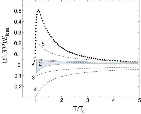
FIG. 6.: The trace anomaly density for pure-glue QCD as a function of $T/T_{c}$. The HTL trace anomaly density is shown as a shaded band that correspond to varying $\mu_{3}$ and $\mu_{4}$ by a factor of two around their central values. The result from differentiating the weak-coupling expansions through order $\alpha_{s}$, $\alpha_{s}^{3/2}$, $\alpha_{s}^{2}$, and $\alpha_{s}^{5/2}$ are shown as dashed lines labeled 2, 3, 4, and 5. The lattice results ofBoyd et al. [4] are shown as diamonds.

The pressure is normalized to the pressure ${\cal P}_{\rm ideal}$ of an ideal gas of massless gluons. The trace anomaly density is normalized to the energy density ${\cal E}_{\rm ideal}=3{\cal P}_{\rm ideal}$ of the ideal gas. The normalized energy density ${\cal E}/{\cal E}_{\rm ideal}$ is given by the sum of the values in Figs. 5 and 6. The interpolation curves are represented by diamonds at a set of discrete points. The size of the diamonds indicates the typical error of about 3% at any single value of $T$.

The leading order HTL results for the pressure and the trace anomaly density are shown in Figs. 5 and 6. We use the expression (113) for the thermal gluon mass, with the running coupling constant given by (115) and with $T_{c}=1.03\Lambda_{\overline{\mbox{MS}}}$. To illustrate the sensitivity to the choices of renormalization scales $\mu_{3}$ and $\mu_{4}$, we take their central values to be

$$\mu_{3}(T) = 0.717m_{g}(T),$$ (117)

$$\mu_{4} = 2\pi T,$$ (118)

and we allow variations by a factor of 2 in the coefficients on the right side of (117) and  (118). The shaded bands in Figs. 5 and 6 indicate the resulting range in the predictions. The ranges are dominated by the variation in $\mu_{4}$ at the largest values of $T$ shown and by the variation in $\mu_{3}$ for $T$ near $T_{c}$. For comparison, the predictions from the QCD weak-coupling expansion (3) with $\mu_{4}=2\pi T$ are also shown in Fig. 5 and Fig. 6. The expansion (3) of the pressure truncated after orders $\alpha_{s}$, $\alpha_{s}^{3/2}$, $\alpha_{s}^{2}$, and $\alpha_{s}^{5/2}$ are shown in Fig. 5 as the dashed lines labeled 2, 3, 4, and 5. The corresponding predictions for the trace anomaly density are shown as dashed lines in Fig. 6. They were obtained by evaluating the derivative in (109) numerically.

The HTL pressure shown in Fig. 5 has the correct shape at the largest values of $T$, but the slope also remains small for $T$ near $T_{c}$. The small slope can be understood from the fact that our expression for $m_{g}(T)$ in (113) is almost linear in $T$. If it were exactly linear in $T$, then ${\cal P}_{\rm HTL}/T^{4}$ would be constant. The factor of the running coupling constant in (113) causes $m_{g}(T)$ to grow a little slower than linear in $T$, which causes ${\cal P}_{\rm HTL}/T^{4}$ to increase slowly with $T$.

The leading order HTL free energy in Fig. 5 lies below the lattice results at the highest temperature available. This deviation has the correct sign and roughly the correct magnitude for the inclusion of the next-to-leading order correction in HTL perturbation theory to give a better approximation to the pressure. The next-to-leading order correction to ${\cal P}_{HTL}/{\cal P}_{\rm ideal}$ should be positive at large $T$, since it must approach $+{15\over 2}\alpha_{s}/\pi$ at asymptotically large temperatures.

The HTL prediction for the trace anomaly in Fig. 6 is very small. The reason for this is that the differentiation in (109) increases the size of the $\alpha_{s}^{3/2}$ term relative to the $\alpha_{s}$ term by a factor of $3/2$. As a consequence there is a near cancellation between the oversubtracted $\alpha_{s}$ term and the $\alpha_{s}^{3/2}$ term. If the next-to-leading order correction in HTL perturbation theory is dominated by the remaining $\alpha_{s}$ term, it would give a negative contribution, increasing the discrepancy with the lattice results. However, the fact that there is a near cancellation at leading order makes it dangerous to predict the effect of the next-to-leading order correction.

D Comparison with Quasiparticle Models

The HTL free energy (65) can be interpreted as essentially that of an ideal gas of gluon quasiparticles, except that it is modified in such a way as to consistently take into account the screening effects of the plasma. It is worthwhile to compare it with the phenomenological quasiparticle models that have been used to describe QCD thermodynamics [16, 17]. In the most recent analyses by Peshier et al. [18] and by Lévai and Heinz [19], the quasiparticle model is an ideal gas of transverse gluons with a temperature-dependent mass. Their expressions for the pressure and energy density are

$${\cal P} = {N_{c}^{2}-1\over 3\pi^{2}}\int_{0}^{\infty}dk\;\left(k^{3}{d\omega_{T}\over dk}\right){1\over e^{\beta\omega_{T}}-1}-B(T),$$ (119)

$${\cal E} = {N_{c}^{2}-1\over\pi^{2}}\int_{0}^{\infty}dk\;k^{2}\omega_{T}{1\over e^{\beta\omega_{T}}-1}+B(T).$$ (120)

The “bag function” $B(T)$, which cancels in the entropy density ${\cal S}=({\cal E}+{\cal P})/T$, is determined up to an integration constant $B_{0}$ by the thermodynamic consistency condition

$${\cal E}=T{d{\cal P}\over dT}-{\cal P}.$$ (121)

The transverse dispersion relation $\omega_{T}$ was taken to be

$$\omega_{T}^{2}=k^{2}+{3\over 2}m_{g}^{2},$$ (122)

which is the solution to (35) in the limit $k\gg m_{g}$.

We now compare the expression (119) for the pressure in the quasiparticle model with the HTL pressure which is the negative of (65). The transverse quasiparticle contributions agree after an integration by parts. The only difference is the use of the simplified dispersion relation (122) instead of the solution to (35), but that is a good approximation in the most important momentum regions. In the quasiparticle model, the contributions from the plasmon, from Landau damping, and from zero-point energies are replaced by the bag function $B(T)$, which is assumed to cancel in the combination ${\cal E}(T)+{\cal P}(T)$. This assumption is not justified within the HTL framework.

In their analysis, Lévai and Heinz determined the mass $m_{g}(T)$ by fitting the lattice results for the pressure ${\cal P}(T)$ [19]. Their result for $m_{g}(T)$ is approximately linear in $T$ between $2T_{c}$ and $4.5T_{c}$, with a coefficient of proportionality of about $0.75$, and it rises to about $3.5T$ as $T$ approaches $T_{c}$. This is qualitatively similar to the behavior predicted by the expression (113) for the thermal gluon mass in the weak-coupling limit. If the scale $\mu_{4}$ in (113) is determined by fitting the lattice results at the highest available temperature near 4.5$T_{c}$, the result is $\mu_{4}\approx 18T$. This is uncomfortably large for the scale of the running coupling constant. This large value of $\mu_{4}$ has a simple explanation from the point of view of HTL perurbation theory. The next-to-leading order contribution to ${\cal P}/{\cal P}_{\rm ideal}$ in HTL perturbation theory will be positive at large $T$ since it must approach $+{15\over 2}\alpha_{s}/\pi$ in the high-temperature limit. Fitting the lattice results without allowing for the next-to-leading order correction would require a smaller value of $m_{g}$ and hence a larger value of $\mu_{4}$. Thus the large value of $\mu_{4}$ obtained in quasiparticle models is an indication that the interaction between the quasiparticles cannot be neglected.

VII Outlook

We have calculated the free energy of a gluon plasma to leading order in HTL perturbation theory. Extending the calculation to include quarks is straightforward. A more challenging problem will be to extend the calculations to next-to-leading order. This requires calculating two-loop diagrams in HTL perturbation theory. Such a calculation is essential in order to demonstrate that HTL perturbation theory avoids the convergence problem that plagues the conventional perturbative expansion.

In the high-temperature limit, the two-loop HTL free energy will agree with the perturbative expansion (3) up to errors of order of $\alpha_{s}^{2}$. The three-loop HTL free energy would agree up to order $\alpha_{s}^{3}\log\alpha_{s}$. In general, the $n$-loop calculation in HTL perturbation theory will include all the $n$-loop contributions from the scale $T$, which scale like $(g^{2})^{n-1}$, and all the $n$-loop contributions from the scale $gT$, which scale like $g^{2+n}$. One limitation of HTL perturbation theory is that it can not be used to calculate the contribution from magnetostatic gluons with momenta of order $g^{2}T$, which first contribute to the free energy at order $g^{6}$. These effects are inherently nonperturbative. It is possible that they could be calculated by a strategy analogous to that used by Kajantie et al. to compute the Debye mass for QCD. The magnetostatic gluons can be described by an effective theory, called magnetostatic QCD (MQCD), which is a pure $SU(N_{c})$ gauge theory in three euclidean dimensions. The parameters of MQCD could perhaps be calculated by HTL perturbation theory, and then the effects of magnetostatic gluons could be calculated nonperturbatively by applying lattice gauge theory methods to MQCD.

In HTL perturbation theory, the leading order quasiparticle dispersion relations are built into the propagator. At next-to-leading order in $g$, the quasiparticle dispersion relations $\omega_{T}^{2}$ and $\omega_{L}^{2}$ have logarithmic infrared divergences proportional to $g^{2}Tm$ that arise from magnetostatic gluons. It would be unwise to build the next-to-leading order dispersion relations into the propagator, because this would introduce a sensitivity to the magnetostatic gluons into the one-loop free energy that would have to be canceled by higher-loop diagrams. The infrared divergences in the next-to-leading order quasiparticle dispersion relations will of course give a divergent contribution to the next-to-leading order free energy through two-loop diagrams that include a one-loop gluon self-energy correction. However, we expect this divergence to be canceled by a divergence in the corresponding Landau-damping contribution.

One of the advantages of HTL perturbation theory is that it can be applied to the real-time processes that are the most promising signatures for the quark-gluon plasma. With the exception of the production of hard dileptons [8], these signatures have been calculated only at leading order in ordinary QCD perturbation theory. There are two reasons to be concerned about the reliability of these calculations. One is that the higher order corrections for the signatures are probably at least as large and unstable as the higher order corrections for the free energy. There is therefore no way to determine the accuracy of the leading order calculation. The other reason for concern is that the conventional weak-coupling expansion does not give a good approximation to the equation of state. The equation of state is needed to infer a temperature $T$ from the energy density of hot hadronic matter, and $T$ is then used as a parameter in the calculation of the signatures. If the method used to calculate the signatures does not reproduce the equation of state, the whole framework is inconsistent. If the next-to-leading order calculation in HTL perturbation theory gives a good approximation to the equation of state, we can have confidence in the predictions for the signatures that are calculated within the same framework.

HTL perturbation theory provides some justification for quasiparticle models of the quark-gluon plasma. However, it goes far beyond those models, because it provides a framework for systematically calculating the effects of interactions between the quasiparticles. This could have an enormous impact on the phenomenology of the quark-gluon plasma, because the physical picture that is suggested by HTL perturbation theory is dramatically different from the conventional picture of the quark-gluon plasma as an almost ideal gas of ultrarelativistic quarks and gluons. In HTL perturbation theory, the quarks and gluons have thermal masses that are comparable to the temperature $T$, so they are only mildly relativistic. This dramatic difference cannot help but have significant phenomenological implications. There have been two previous studies of the effects of quasiparticle masses on the signatures of a quark-gluon plasma. Biró, Lévai and Müller [17] have studied the effect of a massive gluon on the strangeness production in a quark-gluon plasma. They took the $u$ and $d$ quarks to be massless, they neglected the longitudinal mode of the gluon, and they took the transverse mode to have a temperature-independent mass of 500 MeV. They found that the gluon mass enhances the production of $s\bar{s}$ pairs at temperatures below 300 MeV. Additionally, the effects of thermal masses for quarks and gluons on charm production from a quark-gluon plasma has been studied by Lévai and Vogt [23]. They neglected the longitudinal mode of the gluon and took the transverse gluons to have the dispersion relation $\omega_{T}^{2}=k^{2}+m_{g}^{2}$. They found that the thermal masses significantly enhanced the thermal production of charm at RHIC and at LHC.

The previous calculations of the effects of quasiparticle masses have serious theoretical inconsistencies, because introducing a transverse gluon mass by hand destroys gauge invariance. HTL perturbation theory solves this problem by introducing the transverse gluon mass in a gauge-invariant way. But the transverse gluon mass is intricately linked to other essential aspects of relativistic plasma physics, including longitudinal gluons, Landau damping, and the screening of interactions. All of these effects are incorporated consistently within HTL perturbation theory. Thus it provides a foundation for developing a new phenomenology of the quark-gluon plasma in which the many-body aspects of the system play a central role.

A Integrals

In this appendix, we collect the results for the integrals that are required to calculate the one-loop HTL free energy, the first few terms in the high-temperature expansion, and the low-temperature limit. We use dimensional regularization, so that ultraviolet divergences appear as poles in $\epsilon$.

In the HTL free energy, the ultraviolet divergences are isolated in subtraction terms that must be expanded around $\epsilon=0$ through order $\epsilon^{0}$. The integrals required to evaluate the quasiparticle subtractions are

$$\int_{0}^{\infty}dk\;k^{2-2\epsilon}\sqrt{k^{2}+m^{2}} = -{1\over 16}m^{4-2\epsilon}\left[{1\over\epsilon}+2\log 2-{1\over 2}\right],$$ (A.1)

$$\int_{0}^{\infty}dk\;k^{2-2\epsilon}{1\over(k^{2}+m^{2})^{3/2}} = {1\over 2}m^{-2\epsilon}\left[{1\over\epsilon}+2\log 2-2\right],$$ (A.2)

$$\int_{0}^{\infty}dk\;k^{2-2\epsilon}{1\over(k^{2}+m^{2})^{3/2}}\log{k^{2}+m^{2}\over m^{2}} = {1\over 2}m^{-2\epsilon}\left[{1\over\epsilon^{2}}-4+{\pi^{2}\over 6}-2\log^{2}2+4\log 2\right].$$ (A.3)

The corresponding integrals required to evaluate the Landau-damping subtractions are

$$\int_{0}^{\infty}d\omega\;\omega\int_{\omega}^{\infty}dk\;k^{-1-2\epsilon}{k^{2}-\omega^{2}\over k^{2}-\omega^{2}+m^{2}} = -{1\over 4}m^{2-2\epsilon}\left[{1\over\epsilon^{2}}+{\pi^{2}\over 6}\right],$$ (A.4)

$$\int_{0}^{\infty}d\omega\;\omega\int_{\omega}^{\infty}dk\;k^{-3-2\epsilon}{(k^{2}-\omega^{2})^{2}\over(k^{2}-\omega^{2}+m^{2})^{2}} = {1\over 4}m^{-2\epsilon}\left[{1\over\epsilon}-2\right],$$ (A.5)

$$\int_{0}^{\infty}d\omega\;\omega^{2}\int_{\omega}^{\infty}dk\;k^{-4-2\epsilon}{(k^{2}-\omega^{2})^{2}\over(k^{2}-\omega^{2}+m^{2})^{2}}\log{k+\omega\over k-\omega} = {1\over 6}m^{-2\epsilon}\left[{1+2\log 2\over\epsilon}\right.$$ (A.7)

$$\left.+2\log^{2}2-{22\over 3}\log 2-{8\over 3}\right],$$

$$\int_{0}^{\infty}d\omega\;\omega\int_{\omega}^{\infty}dk\;k^{1-2\epsilon}{1\over k^{2}+m^{2}} = -{1\over 4}m^{2-2\epsilon}\left[{1\over\epsilon}\right],$$ (A.8)

$$\int_{0}^{\infty}d\omega\;\omega^{2}\int_{\omega}^{\infty}dk\;k^{-2\epsilon}{1\over(k^{2}+m^{2})^{2}}\log{k+\omega\over k-\omega} = {1\over 6}m^{-2\epsilon}(1+2\log 2)\left[{1\over\epsilon}-1\right].$$ (A.9)

There is also a $T$-dependent integral that multiplies a pole in $\epsilon$ and must therefore be expanded to order $\epsilon$:

$$\int_{0}^{\infty}d\omega\;{\omega^{1-2\epsilon}\over e^{\beta\omega}-1} = {\pi^{2}\over 6}T^{2-2\epsilon}\left[1+\left(2{\zeta^{\prime}(-1)\over\zeta(-1)}-2\log(2\pi)\right)\epsilon\right].$$ (A.10)

There are several nontrivial integrals required to compute the high-temperature expansion and the low-temperature limit for the HTL free energy. One of these integrals is

$$\int_{0}^{\infty}dk\;k^{\alpha}\log(k^{2}+m^{2}) = {\Gamma({\alpha+1\over 2})\Gamma({1-\alpha\over 2})\over\alpha+1}m^{\alpha+1}.$$ (A.11)

This integral with $\alpha=2$ is needed to compute the soft contribution to the free energy from the $n=0$ Matsubara mode. The same integral with $\alpha=3-2\epsilon$ is needed to compute the low-temperature limit of the HTL free energy. In computing the $(m_{g}/T)^{4}$ term in the high-temperature expansion, we need the following infrared-divergent integral:

$$\int_{0}^{\infty}d\omega\;{\omega^{-1-2\epsilon}\over e^{\beta\omega}-1}={1\over 4}\left({1\over\epsilon}+2\gamma-2\log(2\pi)\right).$$ (A.12)

We also need the following integral which comes from changing variables in a momentum integral $x=k/\omega$:

$$\int_{1}^{\infty}dx\;x^{-4-2\epsilon}\log{x+1\over x-1}={1+2\log 2\over 3}+{\pi^{2}-8\log 2-10\over 18}\epsilon.$$ (A.13)

Since it multiplies an infrared pole in $\epsilon$ from the integral (A.12), it must therefore be expanded to order $\epsilon$.

REFERENCES

- [1] P. Arnold and C. Zhai, Phys. Rev. D50, 7603 (1994); Phys. Rev. D51, 1906 (1995);
- [2] B. Kastening and C. Zhai, Phys. Rev. D52, 7232 (1995).
- [3] E. Braaten and A. Nieto, Phys. Rev. Lett. 76, 1417 (1996); Phys. Rev. D53, 3421 (1996).
- [4] G. Boyd et al., Phys. Rev. Lett. 75, 4169 (1995); Nucl. Phys. B469, 419 (1996).
- [5] S. Gottlieb et al., Phys. Rev. D55, 6852 (1997); C. Bernard et al., Phys. Rev. D55, 6861 (1997); J. Engels et al., Phys. Lett. B396, 210 (1997).
- [6] B. Kastening, Phys. Rev. D56, 8107 (1997); T. Hatsuda, Phys. Rev. D56, 8111 (1997).
- [7] E. Braaten, Phys. Rev. Lett. 74, 2164 (1995).
- [8] T. Altherr and P. Aurenche, Z. Phys. C45, 99 (1989).
- [9] K. Kajantie, K. Rummukainen and M. Shaposhnikov, Nucl. Phys. B407, 356 (1993); K. Kajantie, M. Laine, K. Rummukainen and M. Shaposhnikov, Nucl. Phys. B458, 90 (1996).
- [10] K. Kajantie, M. Laine, J. Peisa, A. Rajantie, K. Rummukainen, and M. Shaposhnikov, Phys. Rev. Lett. 79, 3130 (1997).
- [11] R. Parwani and H. Singh, Phys. Rev. D51, 4518 (1995); E. Braaten and A. Nieto, Phys. Rev. D41, 6990 (1995).
- [12] F. Karsch, A. Patkós, and P. Petreczky, Phys. Lett. B401, 69 (1997).
- [13] I.T. Drummond, R.R. Horgan, P.V. Landshoff, and A. Rebhan, Phys. Lett. B398, 326 (1997); Nucl. Phys. B524, 579 (1998); D. Bödeker, P.V. Landshoff, O. Nachtmann, and A. Rebhan, Nucl. Phys. B539, 233 (1998); A. Rebhan, hep-ph/9808480; S. Leupold, hep-ph/9808424.
- [14] S. Chiku and T. Hatsuda, Phys. Rev. D58, 076001 (1998); hep-ph/9809215. S. Chiku and T. Hatsuda, Phys. Rev. D58, 076001 (1998); hep-ph/9809215.
- [15] J.O. Andersen, E. Braaten, and M. Strickland, (in progress).
- [16] F. Karsch, M.T. Mehr, and H. Satz, Z. Phys. C37, 617 (1988); V. Goloviznin and H. Satz, Z. Phys. C57, 671 (1993); A. Peshier, B. Kämpfer, O.P. Pavlenko and G. Soff, Phys. Lett. B337, 235 (1994); M.I. Gorenstein and S.N. Yang, Phys. Rev. D52, 5206 (1995).
- [17] T.S. Biró, P. Lévai and B. Müller, Phys. Rev. D42, 3078 (1990).
- [18] A. Peshier, B. Kämpfer, O.P. Pavlenko, and G. Soff, Phys. Rev. D54, 2399 (1996).
- [19] P. Lévai and U. Heinz, Phys. Rev. C57, 1879 (1998).
- [20] E. Braaten and R.D. Pisarski, Phys. Rev. Lett. 64, 1338 (1990); Nucl. Phys. B337, 569 (1990).
- [21] V.V. Klimov, Sov. Phys. JETP 55, 199 (1982); H.A. Weldon, Phys. Rev. D26, 1394 (1982).
- [22] R. D. Pisarski, Physica A 158, 246 (1989).
- [23] P. Lévai and R. Vogt, Phys. Rev. C56, 2707 (1997).