Off-diagonal quark distribution functions of the pion within an effective single instanton approximation.

I.V. Anikin^ac,   A. E. Dorokhov^ab,   A.E. Maximov^a,   L. Tomio^b,   V. Vento^c

^aBogoliubov Laboratory of Theoretical Physics, Joint Institute for Nuclear Research, Dubna, Russia

anikin@thsun1.jinr.ru

dorokhov@thsun1.jinr.ru

maximov@thsun1.jinr.ru

^b Instituto de Física Teórica, Universidade Estadual Paulista,
São Paulo, Brasil

tomio@ift.unesp.br

^c Departamento de Fisica Teorica and Instituto de Física Corpuscular,
Universidad de Valencia - Consejo Superior de Investigaciones Científicas,
Valencia, Spain

vicente.vento@uv.es

Abstract

We develop a relativistic quark model for pion structure, which incorporates the non-trivial structure of the vacuum of Quantum Chromodynamics as modelled by instantons. Pions are boundstates of quarks and the strong quark-pion vertex is determined from an instanton induced effective lagrangian. The interaction of the constituents of the pion with the external electromagnetic field is introduced in gauge invariant form. The parameters of the model, i.e., effective instanton radius and constituent quark masses, are obtained from the vacuum expectation values of the lowest dimensional quark and gluon operators and the low-energy observables of the pion. We apply the formalism to the calculation of the pion form factor by means of the isovector nonforward parton distributions and find agreement with the experimental data.

Pacs: 11.15.Kc, 12.38.Lg,12.39.Ki,14.65.Bt

Keywords: vacuum, instanton, quark, meson, parton.

1 Introduction

The quark and gluon distribution functions play an important role in the exploration of hadron structure. Perturbative quantum chromodynamics (pQCD) allows one to obtain the evolution of the distribution functions with $Q^{2}$ using operator product expansion and renormalization group methods from some starting input, which cannot be calculated from the first principles. We have been therefore motivated to develop an effective approach which, based on fundamental principles of QCD, serves to estimate the observables associated with the dynamics of large distances.

Recently much attention has been paid to the off-diagonal quark (and gluon) distribution functions parametrizing asymmetrical hadron matrix elements of the light-cone quark-gluon operators. The off-diagonal distribution functions are a generalization of the conventional distribution functions, which serve as a link between the hadronic structure functions and their form factors.

In here, we calculate the isovector off-diagonal leading-twist quark distribution functions for the pion within a novel approach, which is an extension of the well-known instanton model [1]-[4] incorporating bosonization. An effective quark-hadron lagrangian of nonlocal type, where the nonlocality is generated by instantons, underlies our approach. We implement gauge invariance with respect to external electromagnetic field in the effective lagrangian and the Green functions by introducing explicitly the Schwinger phase factor in the definition of quark fields. The parameters of the instanton vacuum, the instanton radius and the constituent quark mass, are related to vacuum expectation values of the lowest dimension quark-gluon operators. The coupling constants are calculated from the compositeness condition which is formulated in our case as the vanishing of the renormalization constant of the meson-field. The quark distribution functions obtained correspond to a hadronic scale (point of normalization) given by the typical relative quark momenta that flows through the instanton vertex and is of order $\mu_{0}\sim p\sim\rho_{c}^{-1}\approx 0.5\div 1\,\,GeV$. We ought to stress that at some point in our development we restrict the calculation to the isovector part of distribution which is the only one required by the scrutinized observable .

We proceed in the next section to describe the nonlocal four-quark model induced by instanton exchange in the effective single instanton approximation.

Section 3 is devoted to fix the parameters of the model from the experimental values of the vacuum condensates and the properties of the pion. In section 4 we calculate the corresponding nonforward parton distributions associated with deeply virtual Compton scattering and determine the pion form factor. In an appendix we explicitly show the contributions from the different diagrams.

2 Model

The investigation of the ground state properties of QCD has important consequences for the description of the hadronic processes within the theory. At present, there exists at least three main approaches for studying the structure of the vacuum: i) the quasi-classical approximation; ii) a formalism based on Wilson’s operator product expansion ; iii) lattice QCD. As it is well-known, the main problem of the quasi-classical method is that, for the $3+1$- dimensional Yang-Mills theory, the instanton gas approximation is not able to provide the correct vacuum-vacuum amplitudes in the background of large QCD-vacuum fluctuations. In a scale-invariant theory, like QCD, the vacuum fluctuations can have large sizes leading to an infinite instanton–anti-instanton medium density, this is the so called infrared divergence problem, which hinders the solution.

At the present, one way for stabilizing the pseudoparticle medium is the instanton liquid model ( see, for example,  [1, 2]). In the framework of instanton liquid model, the medium of $I-\bar{I}$ is quite rarefied, i. e., the ratio of the average size to the average distance between pseudoparticles being approximately equal to $1/3$. Besides, in the limit $(N_{c}\rightarrow\infty)$ the size of all (anti-)instantons is taken to be equal to some average size $\bar{\rho}$. The instanton model with fixed average size of instantons and instanton density is the effective single instanton approximation of the QCD vacuum .

Within the single instanton approximation the chirally invariant nonlocal four-fermion action has the following form [6]

$$S_{4q}=\frac{1}{2}G_{I}\int d^{4}X_{0}\int\prod_{n}d^{4}x_{n}K_{I}(x_{1},x_{2},x_{3},x_{4})$$

$$\left\{\sum_{i}\left[\overline{Q}_{R}(X_{0}-x_{1},X_{0})\Gamma_{i}Q_{L}(X_{0},X_{0}+x_{3})\right]\left[\overline{Q}_{R}(X_{0}-x_{2},X_{0})\Gamma_{i}Q_{L}(X,X+x_{4})\right]\right.$$

$$\left.+(R\leftrightarrow L)\right\}$$ (1)

where $X_{0}$ is the position of the center of the instanton, and the matrix combinations $\Gamma_{i}\times\Gamma_{i}$ are

$$(\tau^{a}\otimes\tau^{a}),\qquad\frac{1}{2\left(2N_{c}-1\right)}(\tau^{a}\sigma_{\mu\nu}\otimes\tau^{a}\sigma_{\mu\nu}),$$ (2)

$\tau^{a}=(1,i\vec{\tau})$ are the matrices characterizing flavor space and $N_{c}=3$ is the number of colors. To ensure the gauge invariance of the nonlocal action (2) with respect to an external electromagnetic $A_{\mu}(z)$ field, we define, following [7, 8], the chiral quark fields with the Schwinger phase factor

$$Q_{R(L)}(x,y)=\frac{1\pm\gamma_{5}}{2}Q(x,y)$$

$$Q(x,y)={\rm exp}\left(-ieQ\int\limits_{x}^{y}dz_{\mu}A^{\mu}(z)\right)q(y)$$

$$Q={\rm diag}\left(\frac{2}{3},-\frac{1}{3},-\frac{1}{3}\right).$$ (3)

In the local limit the action (2) describes quarks interacting through the ’t Hooft vertex [9] and it is invariant under global axial ($q(x)\rightarrow\exp{(i\gamma_{5}\tau\cdot\theta)}q(x)$) and vector ($q(x)\rightarrow\exp{(i\tau\cdot\theta)}q(x)$) transformations, and it anomalously violates the $U_{A}(1)$ symmetry ($q(x)\rightarrow\exp{(i\gamma_{5}\theta)}q(x)$). In what follows we neglect the current quark mass and restrict ourselves only to the nonstrange quark sector. In (2), the kernel of the four-quark interaction $K_{I}(x_{1},x_{2},x_{3},x_{4})$ has the form

$$K_{I}(x_{1},x_{2},x_{3},x_{4})=f(x_{1})f(x_{2})f(x_{3})f(x_{4}),$$ (4)

where $f(x_{i})$ are related to the profile function of the quark zero modes (see below). Morever, this kernel characterizes the range of the nonlocality induced by quark-(anti-)quark instanton interaction, which is determined by the average size of instantons. The latter represents a natural cutoff parameter of the effective low energy theory.

The $4$-fermion nonlocal action (2) is linearized by introducing some auxiliary field interpreted as pion field. Since this bosonization procedure has been elucidated in the literature (see, for details, [10]), let us immediately turn to the linearized effective quark-pion interaction lagrangian in gauge-invariant form which is given by ,

$${\cal L}_{\pi\bar{q}q}^{{\rm int}}(x)=g_{\pi\bar{q}q}\int d\xi_{1}d\xi_{2}f(\xi_{1})f(\xi_{2})\overline{Q}(x+\xi_{1},x)i\gamma_{5}\tau\cdot\pi(x)Q(x,x-\xi_{2}).$$ (5)

The physical pion-quark coupling constant $g_{\pi\bar{q}q}$ is determined from a so-called coupling constant condition [11]

$$Z_{\pi}=1+g^{2}_{\pi\bar{\psi}\psi}\Pi^{\prime}(m_{\pi}^{2})=0,$$ (6)

where $Z_{\pi}$ is the renormalization constant of pion field. The physical consequence of the condition $Z_{\pi}=0$ is that the pion field is always found in a dressed state. Besides, the coupling constant condition is a strong restriction because it implements the dynamics responsible for the formation of the bound state.

Summarizing, lagrangian (5) and the coupling constant condition (6) characterize our approach.

3 Model parameters

We briefly discuss the model parameters (for details, see ref. [12]). Due to the effect of spontaneous breaking of the chiral symmetry, the momentum dependent quark mass $M_{q}(k)$ is dynamically generated. It obeys the well-known gap equation [1] , given by

$$\int\frac{d^{4}k}{(2\pi)^{4}}\frac{f^{2}(k)M_{q}(k)}{k^{2}+M_{q}^{2}(k)}=\frac{n_{c}}{4N_{c}M_{q}},$$ (7)

where $M_{q}(k)$, the momentum dependent quark mass, is defined by the dressed quark propagator:

$$S_{F}^{-1}(p)=\hbox to0.0pt{/\hss}p-M_{q}\tilde{Q}(p),$$ (8)

and, $n_{c}=M_{q}^{2}/G_{I}$ is the density of the instanton medium ($G_{I}$ is the four-fermion interaction constant in (2) and $M_{q}=M_{q}(0)$). The solution of eq.(7) has the form

$$M_{q}(k)=M_{q}\tilde{Q}(k),$$ (9)

where $\tilde{Q}(k)=f^{2}(k)$ is the nonperturbative part of the quark propagator which in the axial gauge is given by

$$\tilde{Q}(p) = \frac{1}{2(2\pi)^{2}}\frac{p^{2}}{\rho_{c}^{2}}\int d^{4}x\ exp{(-ip\cdot x)}Q(x^{2}),\;\;\;\tilde{Q}(0)=1;\;\;\;(p=|p|)\;\;\;,$$ (10)

and

$$Q(x^{2}) = \langle:\bar{q}(0)q(x):\rangle/\langle:\bar{q}(0)q(0):\rangle,\;\;\;\;Q(0)=1\;.$$ (11)

In the axial gauge Eq. (11) coincides with the gauge-invariant correlator in which the quark fields are connected by the Schwinger phase factor. In practical calculation we shall use the approximation for (10, 11) as in ref.[12]

$$f(k)\approx 2\pi\rho_{c}\Biggl{(}2.25\exp\left\{-\rho_{c}|k|\right\}-1.25\exp\left\{-3\rho_{c}|k|\right\}\Biggr{)}.$$ (12)

Given the value of the dynamical mass, one can obtain the value of the quark condensate,

$$\langle\bar{q}q\rangle=\lim_{y\rightarrow x}{\rm tr}S_{F}(x-y)=-4N_{c}\int\frac{d^{4}k}{(2\pi)^{4}}\frac{M_{q}(k)}{k^{2}+M_{q}^{2}(k)},$$ (13)

and the average quark virtuality in the vacuum [14]-[15],

$$\lambda_{q}^{2}\equiv\frac{\langle:\bar{q}D^{2}q:\rangle}{\langle:\bar{q}q:\rangle}=-\frac{4N_{c}}{\langle\bar{q}q\rangle}\int\frac{d^{4}k}{(2\pi)^{4}}k^{2}\frac{M_{q}(k)}{k^{2}+M_{q}^{2}(k)}.$$ (14)

The ratio $\eta=M_{q}^{2}(\lambda_{q}^{2})/\lambda_{q}^{2}$ characterizes the diluteness of the instanton liquid vacuum.

Here, we have to emphasize that in the axial gauge the gauge invariant quantity $M_{q}(k)$ is expressed in terms of the gauge invariant nonlocal codensate (11). Thus, the quark condensate and the average quark virtuality in the vacuum are defined in the gauge invariant manner.

For the moment, it is instructive to consider equations (7) - (14) neglecting $M_{q}^{2}(k)$, compared to $k^{2}$, in the denominator of the integrands. This approximation is justified in the dilute liquid regime where $\langle k^{2}\rangle\sim\lambda_{q}^{2}>>M_{q}^{2}(\lambda_{q}^{2})$. Using the explicit form in the momentum representation of the zero mode in the axial gauge [12] from (13), (14) we have [13]

$$\langle\bar{q}q\rangle=-\frac{2N_{c}M_{q}}{\pi^{4}{\rho_{c}}^{2}},\ \ \ \ \ \lambda_{q}^{2}=2\frac{1}{{\rho_{c}}^{2}}.$$

By inverting these relations, we are able to express the parameters of the instanton vacuum model in terms of the fundamental parameters of the QCD vacuum

$${\rho_{c}}^{2}=\frac{2}{\lambda_{q}^{2}},\ \ \ \ \ \ M_{q}=-\frac{\pi^{4}}{N_{c}}\frac{\langle\bar{q}q\rangle}{\lambda_{q}^{2}}.$$ (15)

¿From these relations the model parameters, $\rho_{c}$ and $M_{q}$, can be estimated in terms of the quark condensate, $\langle\bar{q}q\rangle\approx-(230\ \mbox{MeV})^{3}$ [6] and the average quark virtuality. The latter was estimated using QCD sum rules, $\lambda_{q}^{2}=0.4\pm 0.2\ {\rm GeV}^{2}$ [16], and lattice QCD (LQCD) calculations, which yield $\lambda_{q}^{2}=0.55\pm 0.05\$GeV² [17]. These values lead to $\rho_{c}\approx 2$GeV^-1 and $M_{q}\approx 0.3$GeV. The combined analysis of the vacuum and pion properties confirms such estimates [12] and gives for the allowable range of parameters, $1.5{\rm GeV}^{-1}\leq\rho_{c}\leq 2{\rm GeV}^{-1}$, $0.22{\rm GeV}\leq M_{q}\leq 0.26$GeV. We note that the diluteness condition $\eta=M^{2}(\lambda_{q}^{2})/\lambda_{q}^{2}\ll 1$ is well satisfied within the whole window.

4 Deeply virtual Compton scattering and nonforward parton distributions

Let us consider the deeply virtual Compton scattering (DVCS) within our model. The interest of such investigation is that it defines a procedure to calculate the nonforward parton distributions, which correspond to a generalization of the both, the parton distributions and the hadronic form factors.

During virtual Compton scattering, a pion with momentum $p$ absorbs the virtual photon of momentum $q$, producing an outgoing real photon of momentum $q^{\prime}=q+r$ and a recoiling pion with momentum $p^{\prime}=p-r$. We shall concentrate on the deeply virtual kinematic region of $q$, i.e., the Bjorken limit: $Q^{2}=-q^{2}\rightarrow\infty,\,p\cdot q\rightarrow\infty$ and $Q^{2}/(p\cdot q)$, $t=r^{2}$ finite.

The expression for the Compton scattering amplitude of the photon off the pion, with momenta $p$, $q$ in the initial state and $p^{\prime}$, $q^{\prime}$ in the final state, is given by

$$T_{\mu\nu}(p,q) = \int d\xi_{1}d\xi_{2}d\xi_{3}d\xi_{4}\exp\left(iq\xi_{1}-iq^{\prime}\xi_{2}+ip\xi_{3}-ip^{\prime}\xi_{4}\right)$$ (16)

$$\langle\frac{\delta^{4}S}{\delta A_{\mu}(\xi_{1})\delta A_{\mu}(\xi_{2})\delta M_{(\pi)}(\xi_{3})\delta M_{(\pi)}(\xi_{4})}\rangle_{0}.$$

The $S$-matrix has the standard form

$$S=T\exp\left(i\int dx\left[{\cal L}_{eff}(x)+{\cal L}_{em}(x)\right]\right).$$ (17)

This amplitude corresponds to a set of diagrams drawn in figs. $1$. Fig. 1.1 shows the contribution of the $\sigma$ meson to the process we are calculating, which is small, as can be shown numerically and by $\frac{1}{N}$ counting. Moreover it can also be shown that the diagrams labelled ($c$) and ($d$) are suppressed in the Bjorken limit, therefore we shall only pay attention to the diagrams ($a$) and ($b$). Moreover, diagram ($a$) gives the biggest contribution. The general method for obtaining of the off-diagonal distribution function can be found in [19], [18]. Following these methods, we describe in detail only the contribution of diagram ($a$) to the scattering amplitude in the momentum representation

$$T_{\mu\nu}^{(\Delta)}(p,q) = \frac{g_{\pi\bar{q}q}^{2}}{4\pi^{2}}\int\frac{d^{4}k}{4\pi^{2}i}f(k)f^{2}(k-p)f(k-r)\cdot$$ (18)

$${\rm tr\biggl{(}\gamma_{5}S(k-p)\gamma_{5}S(k)\gamma_{\mu}S(k+q)\gamma_{\nu}S(k-r)\biggr{)}.}$$

In order to obtain the distribution functions, it is convenient to define a special coordinate system (see, for instance [18]) in which light-like vectors $p$ and $q^{\prime}$ are collinear. Then other vectors are expanded in terms of $p$, $\hat{n}\equiv q^{\prime}/(p\cdot q^{\prime})$ and the transverse vectors :

$$p^{\prime}_{\mu}=(1-\zeta)p_{\mu}-\frac{t}{2}\hat{n}_{\mu}+p^{\prime\perp}_{\mu},\quad r_{\mu}=\zeta p_{\mu}+\frac{t}{2}\hat{n}_{\mu}+r^{\perp}_{\mu},$$

$$q_{\mu}=-\zeta p_{\mu}+(p\cdot q)\hat{n}_{\mu}+q^{\perp}_{\mu},\quad\zeta=r_{\parallel}\cdot\hat{n}=1-p^{\prime}\cdot\hat{n},$$

$$p\cdot q=p\cdot q^{\prime}+\frac{t}{2},$$ (19)

where $\zeta$ is the asymmetry parameter which in the Bjorken limit coincides with the Bjorken variable $x_{B}$ for deep-inelastic scattering

$$x_{B}=-\frac{q^{2}}{2pq}=\frac{Q^{2}}{2pq}.$$

Now we insert the given decompositon of $4$-vectors in eq. (18) and carry out the integration over $k$, keeping only terms which are not suppressed in the Bjorken limit. Then, using

$$\int\limits_{-1}^{1}d\tilde{X}\delta(\tilde{X}-k\hat{n})=1,$$ (20)

we obtain for the contribution of diagram ($a$) th the Compton scattering amplitude

$$T_{\mu\nu}^{\Delta}(q,q^{\prime},r)=\frac{1}{2}\left(p_{\mu}\hat{n}_{\nu}+\hat{n}_{\mu}p_{\nu}-g_{\mu\nu}\right)\int dX\frac{1}{X-\zeta}{\cal F}_{\zeta}^{\Delta}(X,t)$$ (21)

where

$${\cal F}_{\zeta}^{\Delta}(X,t)=\frac{1}{2-\zeta}\frac{g_{\pi\bar{q}q}^{2}}{4\pi^{2}}\int\frac{d^{4}k}{2(4\pi^{2}i)}f(k)f^{2}(k-p)f(k-r)$$

$${\rm tr}\biggl{(}\gamma_{5}S(k-p)\gamma_{5}S(k)\hat{n}\cdot\gamma S(k-r)\biggr{)}\delta(X-k\hat{n})+(X\rightarrow\bar{X}).$$ (22)

In a similar manner we obtain the contribution of diagram ($b$) which is given by

$$T_{\mu\nu}^{\circ}(q,q^{\prime},r)=\frac{1}{2}\left(p_{\mu}\hat{n}_{\nu}+\hat{n}_{\mu}p_{\nu}-g_{\mu\nu}\right)\int dX\frac{1}{X-\zeta}{\cal F}_{\zeta}^{\circ}(X,t),$$ (23)

where

$${\cal F}_{\zeta}^{\circ}(X,t) = \frac{1}{2-\zeta}\frac{g_{\pi\bar{q}q}^{2}}{4\pi^{2}}\int\frac{d^{4}k}{4\pi^{2}i}f(k)f^{2}(k+p^{\prime})\int\limits_{0}^{1}d\tau f^{\prime}((k-r\tau)^{2}+r^{2}\tau(1-\tau))$$ (24)

$${\rm tr}\Biggl{(}\gamma_{5}S(k)\gamma_{5}S(k+p^{\prime})\Biggr{)}\Biggl{(}2X-\frac{3}{2}\zeta\Biggr{)}$$

$$\Biggl{(}\delta(X-k\hat{n})+\delta(X-\zeta+k\hat{n})\Biggr{)}+(X\rightarrow\bar{X}).$$

The variable $X$ is the total fraction of the initial hadron momentum $p$ carried by the active quark, and satisfies the kinematical constraint $0\leq X\leq 1$.

In order to calculate the structure integrals in eqs. (4) and (24) we use the $\alpha-$representation for all propagators, the Laplace transform for the nonlocal vertex function $f(k)$ and the integral representation for $\delta-$function. Note that, in the $k-$integrals which appear in the above equations, we use the Euclidean signature, but at the final stage we move back to Minkowski space for the external momenta. In the case of $t=0$ we consider a family of asymmetric distribution functions ${\cal F}_{\zeta}(X)$ whose shapes change with $\zeta$. The $\zeta$ -dependence of the asymmetric function is the main difference with respect to the double distribution function $F(x,y)$ recently introduced in  [19]. The asymmetric function ${\cal F}_{\zeta}(X)$ satisfies the sum-rules,

$$\int\limits_{0}^{1}dX{\cal F}_{\zeta}(X)=1.$$ (25)

This distribution function has the following properties [19]: When the total momentum fraction $X$ of the initial hadron momentum $p$ is larger than the fraction $\zeta$ of the momentum transfer $r$, the function ${\cal F}_{\zeta}(X)$ can be treated as a generalization of the usual distribution function; when $X<\zeta$, the asymmetric function can be treated like a distribution amplitude $\Phi$ of the $\bar{q}q$-states, in our case the pion, with momentum $\zeta p$; besides, for $\zeta=1$, the asymmetric quark distribution function ${\cal F}_{\zeta}(X)$ becomes the pion wave function (see, for example, [20]).

The asymmetric quark distribution functions ${\cal F}_{\zeta}^{\Delta}$ and ${\cal F}_{\zeta}^{\circ}$ are shown in fig. 2.

Finally, the integration of Eqs. (4), (24) over the total momentum fraction $X$ yields the following sum rule:

$$\int\limits_{0}^{1}dX{\cal F}_{\zeta}(X,t)=F_{\pi}(t),$$ (26)

where $F_{\pi}(t)$ is the hadronic form factor normalized to unity. The behavior of the form factor $F_{\pi}(t)$ is shown in fig. 3. Our numerical results are in agreement with experimental data and also coincide with results given by other approaches (see, for example, [21]).

5 Concluding remarks

We have used the instanton liquid model of the QCD vacuum to obtain an effective quark-hadron lagrangian by bosonizing the 4-fermion interaction generated by the instantons. The procedure imposes a coupling constant condition which allows us to calculate the physical value of the quark-hadron interaction constant.

The parameters of the model, related to the properties of the vacuum structure, have been fixed by using the $<\bar{q}q>$ condensate and the average quark virtuality of the vacuum. Furthermore, the pion properties confirm our estimates.

We have considered within the model deeply virtual Compton scattering a procedure which allows the calculation of nonforward parton distributions. We have calculated the asymmetric distribution functions at different asymmetrical parameters ($\zeta$). Finally the integration over the total momentum fraction on the nonforward parton distribution yields the pion form factor. Our results agree with those of other authors and with experiments [22].

This work represents step forward in the direction of deriving a model for hadron structure directly from $QCD$ with well established assumptions. The procedure developed can be generalized to other mesons and to baryons, and the work in this direction is in progress.

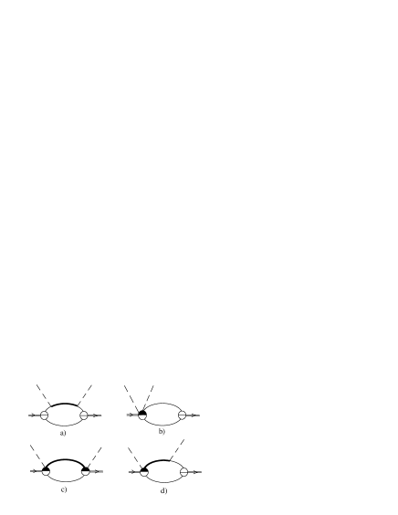
Figure 1: The diagrams contributing to the Compton Scattering amplitude: $(a)$ is the basic type and $(b)-(d)$ are tadpoles.

Figure 2: The sigma exchange diagrams contributing to the Compton Scattering amplitude.

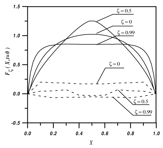
Figure 3: The asymmetric distribution functions at different values of an asymmetry parameter $\zeta$. The solid line shows the contribution to the distribution function of both the basic and the tadpole diagrams; the dashed-line represents the contribution from the tadpoles alone.

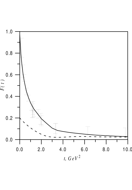
Figure 4: The pion elctromagnetic form factor. The solid line shows the contribution from both the basic and tadpole diagrams, the dashed-line again represents the contribution from the tadpoles only.

References

- [1] D.I.Diakonov, V.Yu.Petrov, Zh.E.T.Ph. 89 (1985) 361.
- [2] D.I.Diakonov, V.Yu.Petrov, Nucl.Phys. B245 (1984) 259.
- [3] E.V.Shuryak, Nucl.Phys. B203 (1982) 93, 116, 140;
- [4] E.V.Shuryak, Nucl.Phys. B214 (1983) 237.
- [5] M.V. Polyakov, C. Weiss, Phys. Rev. D60 (1999) 114017.
- [6] T. Schäfer and E.V. Shuryak, Rev. of Mod. Phys. 70(2), 323 (1998), and references therein.
- [7] S. Mandelstam, Ann. Phys. 19 (1962) 1, 25.
- [8] J. Terning, Phys. Rev. D 44, 887 (1991).
- [9] G. ’t Hooft Phys. Rev. D14 (1976) 3432.
- [10] M.K. Volkov Ann. Phys. (NY) 157 (1984) 228; Sov. J. Part. Nucl. Phys. 17 (1986) 186.
- [11] B. Jouvet Nouvo Cim. 5 (1956) 1133; M.T. Vaughn, R. Aron, R.D. Amado Phys. Rev. 124 (1961) 1258; A. Salam Nouvo Cim. 25 (1962) 224; K. Hayashi et al Fort. der Phys. 15 (1967) 625.
- [12] A.E.Dorokhov, L. Tomio, hep-ph/9803329
- [13] A.E.Dorokhov, S.V.Esaibegyan, S.V.Mikhailov, Phys. Rev. D56 (1997) 4062.
- [14] S.V. Mikhailov and A.V. Radyushkin Sov. J. Nucl. Phys. 49 (1989) 494;
- [15] S.V. Mikhailov and A.V. Radyushkin Phys. Rev. D45 (1992) 1754.
- [16] V.C.Belyaev, B.L.Ioffe Sov. Phys. JETP 56 (1982) 493
- [17] M.Kramer, G.Schierholtz Phys. Lett. B194 (1987) 283
- [18] X.Ji, Phys. Rev. Lett. 78 (1997) 610.
- [19] A.V.Radyushkin, Phys. Rev. D56 (1997) 5524.
- [20] M. Polyakov, Nucl. Phys. B555 (1999) 231.
- [21] I.Anikin et al, Zeit. für Phys. C65 (1995) 681; I.Anikin et al, Phys. of At. Nuclei 57(6) (1994) 1021
- [22] C.J. Bebek et al, Phys. Rev. D17 (1978), 1693.