Abstract

The status of the Higgs boson mass in the Standard Model and its supersymmetric extensions is reviewed and the perspectives of Higgs searches are discussed. The parameter space of the Minimal Supersymmetric Standard Model (MSSM) is analysed with the emphasis on the lightest Higgs mass. The infrared behaviour of renormalization group equations for the parameters of MSSM is examined and infrared quasi-fixed points are used for the Higgs mass predictions. They strongly suggest the Higgs mass to be lighter than 100 or 130 GeV for low and high $\tan\beta$ scenarios, respectively. Extended models, however, allow one to increase these limits for low $\tan\beta$ up to 50%.

1 Introduction

The last unobserved particle from the Standard Model is the Higgs boson. Its discovery would allow one to complete the SM paradigm and confirm the mechanism of spontaneous symmetry breaking. On the contrary, the absence of the Higgs boson would awake doubts about the whole picture and would require new concepts.

The Higgs mechanism is the simplest and minimal mechanism which allows one to provide masses to all the particles of the SM, preserving the renormalizability of a theory. It introduces a single new particle - the Higgs boson, which is considered to be a point-like particle, or a bound state in some approaches, and is supposed to be neutral and massive with the mass of an order of the electroweak breaking scale, i.e. $10^{2}$ GeV.

Experimental limits on the Higgs boson mass come from a direct search at LEP II and Tevatron and from indirect fits of electroweak precision data, first of all from the radiative corrections to the W and top quark masses. A combined fit of modern experimental data gives [2]

$$m_{h}=78^{+86}_{-47}\;{\rm GeV},$$ (1)

which at the 95% confidence level leads to the upper bound of 260 GeV. At the same time, recent direct searches at LEP II for the c.m. energy of 189 GeV give the lower limit of almost 95 GeV[2].

Within the Standard Model the value of the Higgs mass $m_{h}$ is not predicted. The effective potential of the Higgs field at the tree level is

$$V_{eff}=-m^{2}|H|^{2}+\frac{\lambda}{2}(|H|^{2})^{2}.$$ (2)

The minimum of $V_{eff}$ is achieved for non-vanishing v.e.v. of the Higgs field $<H>=v$ equal to $v=m/\sqrt{\lambda}$, which gives the mass $m_{h}=\sqrt{2\lambda}v$ as a function of the vacuum expectation value of the Higgs field, $v$ = 174.1 GeV, and the quartic coupling $\lambda$ which is a free parameter. However, one can get the bounds on the Higgs mass. They follow from the behaviour of the quartic coupling which obeys the following renormalization group equation describing the change of $\lambda$ with a scale:

$$\frac{d\lambda}{dt}=\frac{1}{16\pi^{2}}\left(6\lambda^{2}+6\lambda h_{t}^{2}-6h_{t}^{4}+gauge\ terms\right)$$ (3)

with $t=\ln(Q^{2}/\mu^{2})$. Here $h_{t}$ is the top-quark Yukawa coupling. Since the quartic coupling grows with rising energy indefinitely, an upper bound on $m_{h}$ follows from the requirement that the theory be valid up to the scale $M_{Planck}$ or up to a given cut-off scale $\Lambda$ below $M_{Planck}$ [3]. The scale $\Lambda$ could be identified with the scale at which a Landau pole develops. The upper bound on $m_{h}$ depends mildly on the top-quark mass through the impact of the top-quark Yukawa coupling on the running of the quartic coupling $\lambda$.

On the other hand, the requirement of vacuum stability in the SM (positivity of $\lambda$) imposes a lower bound on the Higgs boson mass, which crucially depends on the top-quark mass as well as on the cut-off $\Lambda$ [3, 4]. Again, the dependence of this lower bound on $m_{t}$ is due to the effect of the top-quark Yukawa coupling on the quartic coupling in eq.(3), which drives $\lambda$ to negative values at large scales, thus destabilizing the standard electroweak vacuum.

From the point of view of LEP and Tevatron physics, the upper bound on the SM Higgs boson mass does not pose any relevant restriction. The lower bound on $m_{h}$, instead, is particularly important in view of search for the Higgs boson at LEPII and Tevatron. For $m_{t}\sim 174$ GeV and $\alpha_{s}(M_{Z})=0.118$ the results at $\Lambda=10^{19}$ GeV or at $\Lambda=1$ TeV can be given by the approximate formulae[4]

$$m_{h} > 135+2.1[m_{t}-174]-4.5\left[\frac{\alpha_{s}(M_{Z})-0.118}{0.006}\right],\ \ \ \ \Lambda=10^{19}\ GeV,$$ (4)

$$m_{h} > 72+0.9[m_{t}-174]-1.0\left[\frac{\alpha_{s}(M_{Z})-0.118}{0.006}\right],\ \ \ \ \Lambda=1\ TeV,$$ (5)

where the masses are in units of GeV.

Fig.1 [5] shows the perturbativity and stability bounds on the Higgs boson mass of the SM for different values of the cut-off $\Lambda$ at which new physics is expected.

Figure 1: Strong interaction and stability bounds on the SM Higgs boson mass. $\Lambda$ denotes the energy scale up to which the SM is valid.

We see from Fig.1 and eqs.(4,5) that indeed for $m_{t}\sim 174$ GeV the discovery of a Higgs particle at LEPII would imply that the Standard Model breaks down at a scale $\Lambda$ well below $M_{GUT}$ or $M_{Planck}$, smaller for lighter Higgs. Actually, if the SM is valid up to $\Lambda\sim M_{GUT}$ or $M_{Planck}$, for $m_{t}\sim 174$ GeV only a small range of values is allowed: $134<m_{h}<\sim 200$ GeV. For $m_{t}$ = 174 GeV and $m_{h}<100$ GeV [i.e. in the LEPII range] new physics should appear below the scale $\Lambda\sim$ a few to 100 TeV. The dependence on the top-quark mass however is noticeable. A lower value, $m_{t}\simeq$ 170 GeV, would relax the previous requirement to $\Lambda\sim 10^{3}$ TeV, while a heavier value $m_{t}\simeq$ 180 GeV would demand new physics at an energy scale as low as 10 TeV.

The previous bounds on the scale at which new physics should appear can be relaxed if the possibility of a metastable vacuum is taken into account [6]. In this case, the lower bounds on $m_{h}$ follow from requiring that no transition at any finite temperature occurs, so that all space remains in the metastable electroweak vacuum. In practice, if the metastability arguments are taken into account, the lower bounds on $m_{h}$ become gradually weaker, though the calculations become less reliable.

On the other hand, this low limit is only valid in the SM with one Higgs doublet: it is enough to add a second doublet with the mass lighter than $\Lambda$ to avoid it. A particularly important example of a theory where the bound is avoided is the Minimal Supersymmetric Standard Model.

2 The Higgs Boson Mass in Minimal Supersymmetry

Supersymmetric extensions of the Standard Model are believed to be the most promising theories at high energies. An attractive feature of SUSY theories is a possibility of unifying various forces of Nature. The best known supersymmetric extension of the SM is the Minimal Supersymmetric Standard Model (MSSM) [7]. The parameter freedom of the MSSM comes mainly from the so-called soft SUSY breaking terms, which are the sources of uncertainty in the MSSM predictions. The most common way of reducing this uncertainty is to assume universality of soft terms, which means an equality of some parameters at a high energy scale. Adopting the universality, one reduces the parameter space to a five-dimensional one [7]: $m_{0}$, $m_{1/2}$, $A$, $\mu$, and $B$. The last two parameters are convenient to trade for the electroweak scale $v^{2}=v_{1}^{2}+v_{2}^{2}$, and $\tan\beta=v_{2}/v_{1}$, where $v_{1}$ and $v_{2}$ are the Higgs field vacuum expectation values.

Contrary to the SM, in the MSSM there are at least two Higgs doublets. At the tree level the Higgs potential containing the neutral components and therefore responsible for the masses of physical scalars has the form

$$V=m_{1}^{2}|H_{1}|^{2}+m_{2}^{2}|H_{2}|^{2}-m_{3}^{2}\left(H_{1}H_{2}+h.c.\right)+\frac{g^{2}+g^{\prime 2}}{8}\left(|H_{1}|^{2}-|H_{2}|^{2}\right)^{2}.$$ (6)

There are five physical eigenstates: $CP$-even Higgses $h$ and $H$, $CP$-odd Higgs $A$ and a pair of charged Higgses $H^{\pm}$, which at tree level have the following masses

$$m_{A}^{2} = m_{1}^{2}+m_{2}^{2}\ ,$$

$$m_{h,H}^{2} = \frac{1}{2}\left[m_{A}^{2}+M_{Z}^{2}\mp\sqrt{\left(m_{A}^{2}+M_{Z}^{2}\right)^{2}-4m_{A}^{2}M_{Z}^{2}\cos^{2}2\beta}\right]\ ,$$ (7)

$$m_{H^{\pm}}^{2} = m_{A}^{2}+M_{W}^{2}\ .$$

For $m_{A}\gg M_{Z}$ the mass of the lightest Higgs is less than the $Z$ boson mass

$$m_{h}\simeq M_{Z}|\cos 2\beta|,$$ (8)

independently of any other parameters. However, the inequality $m_{h}<M_{Z}$ is violated by radiative corrections, and the lightest Higgs mass can exceed a hundred GeV, but not very much [8, 9].

The detailed analysis of the MSSM parameter space can be performed by minimization of a $\chi^{2}$ function. This analysis implies also that a number of constraints on the parameters like the gauge coupling unification, $b-\tau$ unification, radiative electroweak symmetry breaking, dark matter density, $b\to s\gamma$ decay rate, etc are imposed. Details of this analysis can be found in Ref. [10, 11].

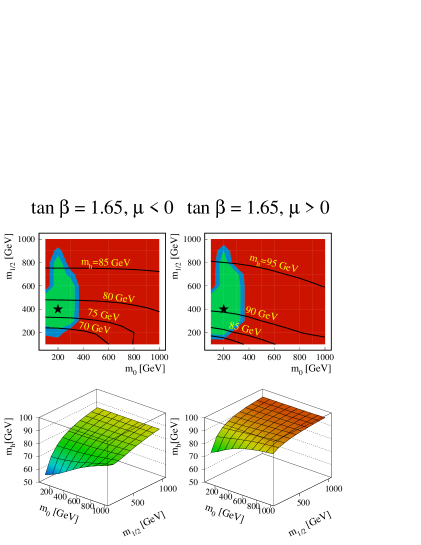
Figure 2: Contours of the Higgs mass (solid lines) in the $m_{0},m_{1/2}$ plane (above) and the Higgs masses (below) for both signs of $\mu$ for the low $\tan\beta$ solution $\tan\beta=1.65$ for $m_{t}=175$ GeV.

For low $\tan\beta$ the present Higgs limit severely constrains the parameter space, as can be seen from Fig. 2, which shows the excluded regions in the ($m_{0},m_{1/2})$ plane for different signs of $\mu$. The experimental Higgs limit of 90 GeV is valid for the low $\tan\beta$ scenario ($\tan\beta<4$) of the MSSM too. As is apparent from Fig. 2 this limit clearly rules out the $\mu<0$ solution, in agreement with other studies [12]. However, this figure assumes $m_{t}=175$ GeV. The top dependence on the Higgs mass is slightly steeper than linear in this range and may move the contours within $\pm 5$ GeV.

Adding about one $\sigma$ to the top mass, i.e. $m_{t}=180$ GeV, implies that for the contours in Fig. 2 one should add 6 GeV to the numbers shown. Even in this case the $\mu<0$ solution is excluded for a large region of the parameter space. Only the small allowed region with $m_{1/2}>700$ GeV is still available for $m_{t}=180$ GeV. Note that in this region the squarks are well above 1 TeV, so in this case the cancellation of the quadratic divergencies in the Higgs masses, which is only perfect if sparticles and particles have the same masses, starts to become worrying again.

For $\mu>0$ practically the whole plane is allowed, except for the left bottom corner shown on the top right-hand side of Fig. 2, although the latest experiment has almost covered this region [2].

The upper limit for the mass of the lightest Higgs is reached for heavy squarks, but it saturates quickly, as is apparent from the bottom row in Fig. 2. For $m_{0}=1000,m_{1/2}=1000$, which corresponds to squarks masses of about 2 TeV, one finds for the upper limit on the Higgs mass in the low $\tan\beta$ scenario [13]:

$$m_{h}^{max}=97\pm 6~{}{\rm GeV},$$

where the error is dominated by the uncertainty from the top mass. If one requires the squarks to be below 1 TeV, these upper limits are reduced by 4 GeV.

For high $\tan\beta$ the upper limit on the Higgs mass in the Constrained MSSM is [13]

$$m_{h}^{max}=120\pm 2~{}{\rm GeV}.$$

The error from the top mass is small since the high $\tan\beta$ fits anyway prefer top masses around 190 GeV.

3 Infrared Quasi-Fixed Point Scenario

One of the possible ways to reduce the parameter freedom of the MSSM is to use the fact that some low-energy parameters are insensitive to their initial high-energy values. This allows one to find them without detailed knowledge of physics at high energies. To do this one has to examine the infrared behaviour of renormalization group equations (RGEs) for these parameters and use possible infrared fixed points to further restrict them. Notice, however, that the true IR fixed points, discussed e.g. in Ref. [14] are reached only in the asymptotic regime. More interesting is another possibility connected with so-called infrared quasi-fixed points (IRQFPs) first discussed in Ref. [15] and then widely studied by other authors [16]-[29]. These fixed points usually give the upper (or lower) bounds for the relevant solutions.

The well-known example of such infrared behaviour is the top-quark Yukawa coupling $Y_{t}=h_{t}/(4\pi)^{2}$ for low $\tan\beta$ in the framework of the MSSM. In this case the corresponding one-loop RGE has exact solution

$$Y_{t}(t)=\frac{Y_{0t}E(t)}{1+6Y_{0t}F(t)},$$ (9)

where $E(t)$ and $F(t)$ are some known functions. It exhibits the IRQFP behaviour in the limit $Y_{0t}=Y_{t}(0)\to\infty$ [15, 18, 19, 20, 22, 30] where the solution becomes independent of the initial conditions:

$$Y_{t}(t)\Rightarrow Y_{t}^{FP}=\frac{E(t)}{6F(t)}.$$ (10)

A similar conclusion is valid for the other couplings [20, 22, 23, 24, 29, 30]. It has been pointed out that the IRQFPs exist for the trilinear SUSY breaking parameter $A_{t}$ [22], for the squark masses [20, 23] and for the other soft supersymmetry breaking parameters in the Higgs and squark sector [29].

In the case of large $\tan\beta$ the system of the RGEs has no analytical solution and one can use either numerical or approximate ones. It has been shown [31] that almost all SUSY breaking parameters exhibit IRQFP behaviour.

For the IRQFP solutions the dependence on initial conditions $Y_{i0},A_{0}$ and $m_{0}$ disappears at low energies. This allows one to reduce the number of unknown parameters and make predictions for the MSSM particle masses as functions the only free parameter, namely $m_{1/2}$, or the gaugino mass, while the other parameters are strongly restricted.

The strategy is the following [32, 31]. As input parameters one takes the known values of the top-quark, bottom-quark and $\tau$-lepton masses ($m_{t},m_{b},m_{\tau}$), the experimental values of the gauge couplings [2] $\alpha_{3}=0.118,\alpha_{2}=0.034,\alpha_{1}=0.017$, the sum of Higgs vev’s squared $v^{2}=v_{1}^{2}+v_{2}^{2}=(174.1\ GeV)^{2}$ and the fixed-point values for the Yukawa couplings and SUSY breaking parameters. To determine $\tan\beta$ the relations between the running quark masses and the Higgs v.e.v.s in the MSSM are used

$$m_{t} = h_{t}\ v\ \sin\beta\,,$$ (11)

$$m_{b} = h_{b}\ v\ \cos\beta\,,$$ (12)

$$m_{\tau} = h_{\tau}\ v\ \cos\beta\,.$$ (13)

The Higgs mixing parameter $\mu$ is defined from the minimization conditions for the Higgs potential. Then, one is left with a single free parameter, namely $m_{1/2}$, which is directly related to the gluino mass $M_{3}$. Varying this parameter within the experimentally allowed range, one gets all the masses as functions of this parameter.

For low $tan\beta$ the value of $\sin\beta$ is determined from eq.(11), while for high $\tan\beta$ it is more convenient to use the relation $\tan\beta=\frac{m_{t}}{m_{b}}\frac{h_{b}}{h_{t}}$, since the ratio $h_{t}/h_{b}$ is almost a constant in the range of possible values of $h_{t}$ and $h_{b}$.

For the evaluation of $\tan\beta$ one first needs to determine the running top- and bottom-quark masses. One can find them using the well-known relations to the pole masses (see e.g. [33, 34, 30]), including both QCD and SUSY corrections. For the top-quark one has:

$$m_{t}(m_{t})=\frac{m_{t}^{pole}}{1+\left(\frac{\Delta m_{t}}{m_{t}}\right)_{QCD}+\left(\frac{\Delta m_{t}}{m_{t}}\right)_{SUSY}},$$ (14)

where $m_{t}^{pole}=(174.1\pm 5.4)$ GeV [35]. Then, the following procedure is used to evaluate the running top mass. First, only the QCD correction is taken into account and $m_{t}(m_{t})$ is found in the first approximation. This allows one to determine both the stop masses and the stop mixing angle. Next, having at hand the stop and gluino masses, one takes into account the stop/gluino corrections.

For the bottom quark the situation is more complicated because the mass of the bottom quark $m_{b}$ is essentially smaller than the scale $M_{Z}$ and so one has to take into account the running of this mass from the scale $m_{b}$ to the scale $M_{Z}$. The procedure is the following [34, 36, 37]: one starts with the bottom-quark pole mass, $m_{b}^{pole}=4.94\pm 0.15$ [38] and finds the SM bottom-quark mass at the scale $m_{b}$ using the two-loop $QCD$ corrections

$$m_{b}(m_{b})^{SM}=\frac{m_{b}^{pole}}{1+\left(\frac{\Delta m_{b}}{m_{b}}\right)_{QCD}}\,.$$ (15)

Then, evolving this mass to the scale $M_{Z}$ and using a numerical solution of the two-loop SM RGEs [34, 37] with $\alpha_{3}(M_{Z})=0.12$ one obtains $m_{b}(M_{Z})_{SM}=2.91$ GeV. Using this value one can calculate the sbottom masses and then return back to take into account the SUSY corrections from massive SUSY particles

$$m_{b}(M_{Z})=\frac{m_{b}(M_{Z})^{SM}}{1+\left(\frac{\Delta m_{b}}{m_{b}}\right)_{SUSY}}\,.$$ (16)

When calculating the stop and sbottom masses one needs to know the Higgs mixing parameter $\mu$. For determination of this parameter one uses the relation between the $Z$-boson mass and the low-energy values of $m_{H_{1}}^{2}$ and $m_{H_{2}}^{2}$ which comes from the minimization of the Higgs potential:

$$\frac{M_{Z}^{2}}{2}+\mu^{2}=\frac{m_{H_{1}}^{2}+\Sigma_{1}-(m_{H_{2}}^{2}+\Sigma_{2})\tan^{2}\beta}{\tan^{2}\beta-1}\,,$$ (17)

where $\Sigma_{1}$ and $\Sigma_{2}$ are the one-loop corrections [11]. Large contributions to these functions come from stops and sbottoms. This equation allows one to obtain the absolute value of $\mu$, the sign of $\mu$ remains a free parameter.

Whence the quark running masses and the $\mu$ parameter are found, one can determine the corresponding values of $\tan\beta$ with the help of eqs.(11,12). This gives in low and high $\tan\beta$ cases, respectively

$$\tan{\beta} = 1.47\pm 0.15\pm 0.05\ \ \ for\ \mu>0\,,$$

$$\tan{\beta} = 1.56\pm 0.15\pm 0.05\ \ \ for\ \mu<0\,,$$

$$\tan{\beta} = 76.3\pm 0.6\pm 0.3\ \ \ \ \ for\ \mu>0\,,$$

$$\tan{\beta} = 45.7\pm 0.9\pm 0.4\ \ \ \ \ for\ \mu<0\,.$$

The deviations from the central value are connected with the experimental uncertainties of the top-quark mass, $\alpha_{3}(M_{Z})$ and uncertainty due to the fixed point values of $h_{t}(M_{Z})$ and $h_{b}(M_{Z})$.

Having all the relevant parameters at hand it is possible to estimate the masses of the Higgs bosons. With the fixed point behaviour one has the only dependence left, namely on $m_{1/2}$ or the gluino mass $M_{3}$. It is restricted only experimentally: $M_{3}>144$ GeV [2] for arbitrary values of the squarks masses.

Let us start with low $\tan\beta$ case. The masses of CP-odd, charged and CP-even heavy Higgses increase almost linearly with $M_{3}$. The main restriction comes from the experimental limit on the lightest Higgs boson mass. It excludes $\mu<0$ case and for $\mu>0$ requires the heavy gluino mass $M_{3}\geq 750$ GeV. Subsequently one obtains

$$m_{A}>844\ GeV,\ \ m_{H^{\pm}}>846\ GeV,\ \ m_{H}>848\ GeV,\ \ \ for\ \mu>0,$$

i.e. these particles are too heavy to be detected in the nearest experiments.

For high $\tan\beta$ already the requirement of positivity of $m_{A}^{2}$ excludes the region with small $M_{3}$. In the most promising region $M_{3}>1$ TeV ($m_{1/2}>300$ GeV) for the both cases $\mu>0$ and $\mu<0$ the masses of CP-odd, charged and CP-even heavy Higgses are also too heavy to be detected in the near future

$$m_{A}>1100\ \mbox{GeV for}\ \ \mu>0,\ \ \ m_{A}>570\ \mbox{GeV for}\ \ \mu<0,$$

$$m_{H^{\pm}}>1105\ \mbox{GeV for}\ \ \mu>0,\ \ \ m_{H^{\pm}}>575\ \mbox{GeV for}\ \ \mu<0.$$

$$m_{H}>1100\ \mbox{GeV for}\ \ \mu>0,\ \ \ m_{H}>570\ \mbox{GeV for}\ \ \mu<0.$$

The situation is different for the lightest Higgs boson $h$, which is much lighter. As has been already mentioned, for low $\tan\beta$ the negative values of $\mu$ are excluded by the experimental limits on the Higgs mass. Further on we consider only the positive values of $\mu$. Fig. 3 shows the value of $m_{h}$ for $\mu>0$ as a function of the geometrical mean of stop masses - this parameter is often identified with a supersymmetry breaking scale $M_{SUSY}$. One can see that the value of $m_{h}$ quickly saturates close to $\sim$ 100 GeV. For $M_{SUSY}$ of the order of 1 TeV the value of the lightest Higgs mass is [32]

$$m_{h}=(94.3+1.6+0.6\pm 5\pm 0.4)\ \mbox{GeV},\ \ \ \mbox{ for}\ M_{SUSY}=1\ TeV,$$ (18)

where the first uncertainty comes from the deviations from the IRQFPs for the mass parameters, the second one is related to that of the top-quark Yukawa coupling, the third reflects the uncertainty of the top-quark mass of 5.4 GeV, and the last one comes from that of the strong coupling.

One can see that the main source of uncertainty is the experimental error in the top-quark mass. As for the uncertainties connected with the fixed points, they give much smaller errors of the order of 1 GeV.

Note that the obtained result (18) is very close to the upper boundary, $m_{h}=97$ GeV, obtained in Refs. [30, 13] (see the previous section).

For the high $\tan\beta$ case the lightest Higgs is slightly heavier, but the difference is crucial for LEP II. The mass of the lightest Higgs boson as a function of $M_{SUSY}$ is shown in Fig.3. One has the following values of $m_{h}$ at a typical scale $M_{SUSY}=1$ TeV ($M_{3}\approx 1.3$TeV) [31]:

$$m_{h} = 128.2-0.4-7.1\pm 5\ \mbox{GeV, \ for}\ \mu>0\,,$$

$$m_{h} = 120.6-0.1-3.8\pm 5\ \mbox{GeV,\ for}\ \mu<0\,.$$

The first uncertainty is connected with the deviations from the IRQFPs for mass parameters, the second one with the Yukawa coupling IRQFPs, and the third one is due to the experimental uncertainty in the top-quark mass. One can immediately see that the deviations from the IRQFPs for mass parameters are negligible and only influence the steep fall of the function on the left, which is related to the restriction on the CP-odd Higgs boson mass $m_{A}$. In contrast with the low $\tan\beta$ case, where the dependence on the deviations from Yukawa fixed points was about $1$ GeV, in the present case it is much stronger. The experimental uncertainty in the strong coupling constant $\alpha_{s}$ is not included because it is negligible compared to those of the top-quark mass and the Yukawa couplings and is not essential here contrary to the low $\tan\beta$ case.

One can see that for large $\tan\beta$ the masses of the lightest Higgs boson are typically around 120 GeV that is too heavy for observation at LEP II.

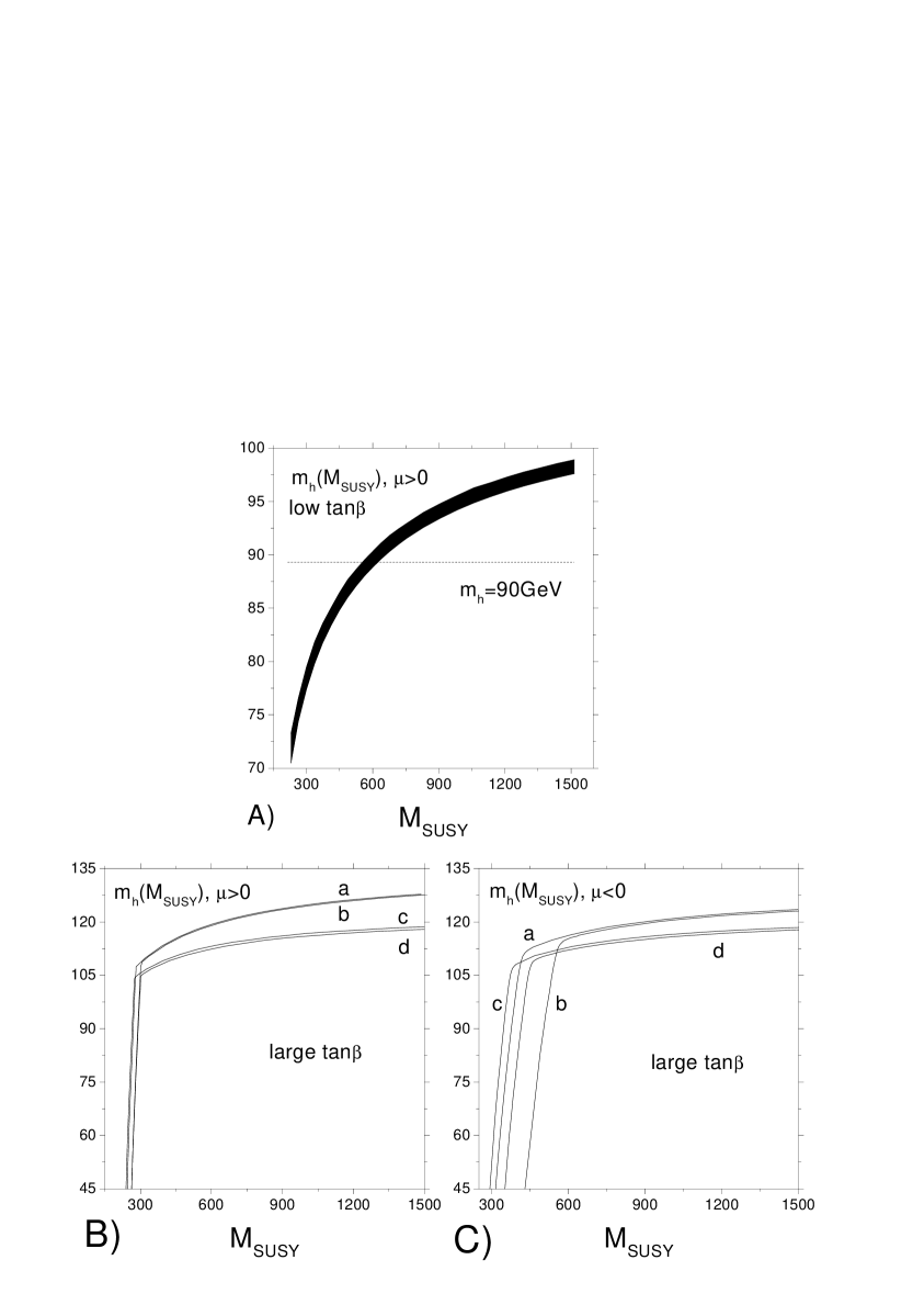
Figure 3: A) The dependence of the mass of the lightest Higgs boson $h$ on $M_{SUSY}=(\tilde{m}_{t_{1}}\tilde{m}_{t_{2}})^{1/2}$ (shaded area) for $\mu>0$, low $\tan\beta$. The dashed line corresponds to the minimum value of $m_{h}=90$ GeV allowed by experiment. B),C) The mass of the lightest Higgs boson $h$ as function of $M_{SUSY}$ for different signs of $\mu$, large $\tan\beta$. The curves (a,b) correspond to the upper limit of the Yukawa couplings and to $m_{0}^{2}/m_{1/2}^{2}=0$ (a) or to $m_{0}^{2}/m_{1/2}^{2}=2$ (b). The curves (c,d) correspond to the lower limit of the Yukawa couplings and to $m_{0}^{2}/m_{1/2}^{2}=0$ (c) or to $m_{0}^{2}/m_{1/2}^{2}=2$ (d). Possible values of the mass of the lightest Higgs boson are inside the areas marked by these lines.

4 Summary and Conclusion

Thus, one can see that in the IRQFP approach all the Higgs bosons except for the lightest one are found to be too heavy to be accessible in the nearest experiments. This conclusion essentially coincides with the results of more sophisticated analyses. The lightest neutral Higgs boson, on the contrary is always light. In the case of low $\tan\beta$ its mass is small enough to be detected or excluded in the next two years when the c.m.energy of LEP II reaches 200 GeV. On the other hand, for the high $\tan\beta$ scenario the values of the lightest Higgs boson mass are typically around 120 GeV, which is too heavy for the observation at LEP II leaving hopes for the Tevatron and LHC.

However, these SUSY limits on the Higgs mass may not be so restricting if non-minimal SUSY models are considered. In a SUSY model extended by a singlet, the so-called Next-to-Minimal model, eq.(8) is modified and at the tree level the bound looks like [39]

$$m_{h}^{2}\simeq M_{Z}^{2}\cos^{2}2\beta+\lambda^{2}v^{2}\sin^{2}2\beta,$$ (19)

where $\lambda$ is an additional singlet Yukawa coupling. This coupling being unknown brings us back to the SM situation, though its influence is reduced by $\sin 2\beta$. As a result, for low $\tan\beta$ the upper bound on the Higgs mass is slightly modified (see Fig.4).

Even more dramatic changes are possible in models containing non-standard fields at intermediate scales. These fields appear in scenarios with gauge mediated supersymmetry breaking. In this case, anyway the upper bound on the Higgs mass may increase up to 155 GeV [39] (the upper curve in Fig.4), though it is not necessarily saturated. One should notice, however, that these more sophisticated models do not change the generic feature of SUSY theories, the presence of the light Higgs boson.

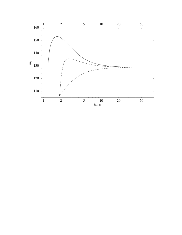
Figure 4: Dependence of the upper bound on the lightest Higgs boson mass on $\tan\beta$ in MSSM (lower curve), NMSSM (middle curve) and extended SSM (upper curve) [39]

Acknowledgments

The author is grateful to A.V.Gladyshev and M.Jurčišin for useful discussions and help in preparing the manuscript. Financial support from RFBR grant # 98-02-17453 is acknowledged.

References

- [1] L.B.Okun’, Uspekhi Fiz. Nauk. 168 (1998) 625.
-
[2]
LEP Electroweak Working Group, CERN-EP/99-15, 1999,
http://www.cern.ch/LEPEWWG/lepewpage.html. -
[3]
N.Cabibbo, L.Maiani, G.Parisi, and R.Petronzio, Nucl. Phys. B158
(1979) 295;
M.Lindner, Z.Phys.C31 (1986) 295; M.Sher, Phys.Rev. D 179 (1989) 273; M.Lindner, M.Sher and H.W.Zaglauer, Phys.Lett. B228 (1989) 139. -
[4]
M.Sher, Phys.Lett. B317 (1993) 159; C.Ford,
D.R.T.Jones, P.W.Stephenson and M.B.Einhorn, Nucl.Phys. B395
(1993) 17;
G.Altarelli and I. Isidori, Phys.Lett. B337 (1994) 141; J.A.Casas, J.R.Espinosa and M.Quiros, Phys.Lett. 342 (1995) 171. - [5] T.Hambye, K.Reisselmann, Phys.Rev. D55 (1997) 7255; H.Dreiner, hep-ph/9902347.
- [6] G.Anderson, Phys.Lett B243 (1990) 265; P.Arnold and S.Vokos, Phys.Rev. D44 (1991) 3260; J.R.Espinosa and M.Quiros, Phys.Lett. 353 (1995) 257.
-
[7]
H.P.Nilles, Phys.Rep. 110 (1984) 1,
H.E.Haber and G.L.Kane, Phys.Rep. 117 (1985) 75;
A.B.Lahanas and D.V.Nanopoulos, Phys.Rep. 145 (1987) 1;
R.Barbieri, Riv.Nuo.Cim. 11 (1988) 1;
W.de Boer, Progr. in Nucl. and Particle Phys. 33 (1994) 201;
D.I.Kazakov, Surveys in High Energy Physics, 10 (1997) 153. - [8] A. Brignole, J. Ellis, G. Ridolfi and F. Zwirner, Phys. Lett. B271 (1991) 123.
- [9] M.Carena, M.Quiros, C.E.M.Wagner, Nucl.Phys. B461 (1996) 407.
- [10] W.de Boer, R.Ehret and D.Kazakov, Z.Phys. C67 (1995) 647; W.de Boer, et al., Z.Phys. C71 (1996) 415.
- [11] A.V.Gladyshev, D.I.Kazakov, W.de Boer, G.Burkart and R.Ehret, Nucl. Phys. B498 (1997) 3.
- [12] S.A.Abel and B.C.Allanach, hep-ph/9803476.
- [13] W.de Boer, H.-J.Grimm, A.V.Gladyshev and D.I.Kazakov, Phys.Lett. B438 (1998) 281.
- [14] B.Pendleton and G.Ross, Phys.Lett. B98 (1981) 291.
-
[15]
C.T.Hill, Phys.Rev. D24 (1981) 691,
C.T.Hill, C.N.Leung, and S.Rao, Nucl.Phys. B262 (1985) 517. -
[16]
E.Paschos, Z.Phys. C26 (1984) 235;
J.Halley, E.Paschos, H.Usler, Phys.Lett. B155(1985) 107. -
[17]
J.Bagger, S.Dimopoulos, E.Masso, Nucl.Phys. B253
(1985) 397 ;
J.Bagger, S Dimopoulos, E.Masso, Phys.Lett. B156 (1985) 357 ;
S.Dimopoulos, S.Theodorakis, Phys.Lett B154 (1985) 153 - [18] W.Barger, M.Berger, P.Ohman, Phys.Lett. B314 (1993) 351
- [19] P.Langacker, N.Polonsky, Phys.Rev. D49 (1994) 454
- [20] M.Carena et al, Nucl.Phys. B419 (1994) 213
- [21] W.Bardeen et al, Phys.Lett. B320 (1994) 110.
- [22] P.Nath et al., Phys.Rev. D52 (1995) 4169.
- [23] M.Carena, C.E.M.Wagner, Nucl.Phys. B452 (1995) 45.
- [24] M.Lanzagorta, G.Ross, Phys. Lett. B364 (1995) 163.
-
[25]
J. Feng, N. Polonsky and S. Thomas, Phys. Lett. B370
(1996) 95,
N. Polonsky, Phys. Rev. D54 (1996) 4537. - [26] B. Brahmachari, Mod. Phys. Lett. A12 (1997) 1969.
- [27] P. Chankowski and S. Pokorski, hep-ph/9702431, in Perspectives on Higgs Physics II, edited by G.L. Kane (World Scientific, Singapure, 1998).
- [28] I. Jack, D.R.T. Jones and K.L. Roberts Nucl. Phys. B455 (1995) 83, P.M. Ferreira, I. Jack and D.R.T. Jones Phys. Lett. B357 (1995) 359.
- [29] S.A.Abel, B.C.Allanach, Phys. Lett. B415 (1997) 371.
- [30] J.Casas, J.Espinosa, H.Haber, Nucl.Phys. B526 (1998) 3.
- [31] M.Jurčišin and D.I.Kazakov, Mod. Phys.Lett A14 (1999) 671, hep-ph/9902290.
- [32] G.K.Yeghiyan, M.Jurčišin and D.I.Kazakov, Mod. Phys.Lett A14 (1999) 601, hep-ph/9807411.
- [33] B.Schrempp, M.Wimmer, Prog.Part.Nucl.Phys. 37 (1996) 1.
-
[34]
D.M.Pierce, J.A.Bagger, K.Matchev and R.Zhang,
Nucl.Phys. B491 (1997) 3,
J.A.Bagger, K.Matchev and D.M.Pierce, Phys.Lett. B348 (1995) 443. - [35] M.Jones, for the CDF and D0 Coll., talk at the XXXIIIrd Recontres de Moriond, (Electroweak Interactions and Unified Theories), Les Arcs, France, March 1998;
- [36] H.Arason, D.Castano, B.Keszthelyi, S.Mikaelian, E.Piard, P.Ramond, and B.Wright, Phys.Rev. D46 (1992) 3945.
- [37] N.Gray, D.J.Broadhurst, W.Grafe, and K.Schilcher, Z.Phys. C48 (1990) 673.
- [38] C.T.H.Davies, et al., Phys.Rev. D50 (1994) 6963.
- [39] M.Masip, R.Munos and A.Pomarol, Phys.Rev. D57 (1998) 5340.