Abstract

We calculate the ratios E2/M1 and C2/M1 for the electroproduction of the $\Delta(1232)$ in the region of photon virtuality $0\!<\!\!-q^{2}\!<\!1\,\,\mbox{GeV}^{2}$. The magnetic dipole amplitude M1 is also presented. The theory used is the chiral quark-soliton model, which is based on the instanton vacuum of the QCD. The calculations are performed in flavours SU(2) and SU(3) taking rotational ($1/N_{c}$) corrections into account. The results for the ratios agree qualitatively with the available data, although the magnitude of both ratios seems to underestimate the latest experimental results.

PACS numbers: 12.39Fe; 13.40-f; 14.20-c
Keywords: Chiral quark-soliton model; Delta electroproduction

1 Introduction

Electromagnetic processes have always played an important part in understanding the structure of the nucleon. Among these processes, the electroproduction of the $\Delta(1232)$ deserves a special place. In fact, from the viewpoint of the simplest quark model, the process $\gamma^{\ast}N\rightarrow\Delta$ is expected to proceed through the spin flip of one of the quarks, which implies a non-vanishing magnetic dipole transition and vanishing quadrupole transition amplitudes. This contradicts the experimental observations of non-vanishing quadupole amplitudes, although small when compared to the magnetic dipole amplitude.

The fact that the first available data [1, 2] for the ratios of electric and coulomb quadrupole amplitudes to the magnetic dipole amplitude, E2/M1 and C2/M1 respectively, did not establish a definite picture for these ratios, motivated in recent years a renewed interest in measurements of such electroproduction amplitudes, mainly due to favourable conditions offered by new experimental facilities like MAMI (Mainz), ELSA-ELAN (Bonn), LEGS (BNL), Bates (MIT) and the Jefferson Laboratory (Newport News). Results coming from these recent experimental activities are expected to allow for a great improvement in the experimental knowledge of the ratios E2/M1 and C2/M1, as [3, 4, 5] let anticipate.

The difference between the quark model predictions and experiment caused intensive discussions on the structure of the nucleon, the delta and the transition density. This process has been studied in the context of many models of baryon structure, which made an overall correct description of these ratios to become a constraint in model-making and refining. In the context of the quark model, to accomodate these noticeable amplitude ratios, charge deformations due to d-state admixtures in non-relativistic and relativized models have been invoked for an explanation [6, 7]. Other explanations can nevertheless be found: it has recently been estimated in photoproduction [8], that the proper consideration of two-body exchange currents alone can give raise to non-vanishing quadrupole amplitudes. Other quark model formulations, like a quark model constructed in the infinite momentum frame [9], a light-front constituent quark model [10] and a three-body force model [11], have also been used in addressing the $\Delta(1232)$ electroproduction amplitudes and/or form factors.

Calculations regarding the electroproduction of the $\Delta(1232)$ were also carried out in the framework of models fully based on chiral symmetry such as the $\sigma$- and chromodielectric models [12], the Skyrme model [13], the cloudy bag model [14] and also in heavy baryon chiral perturbation theory [15], with a recent work [16] extending it. Another class of models is based on effective lagrangian densities containing, to different extents, ingredients like Born terms, vector mesons and nucleon resonances (see [17] and references therein).

It is the aim of this paper to study the ratios E2/M1 and C2/M1 and their momentum dependence for the electroprodution of the $\Delta(1232)$ in the chiral quark-soliton model (CQSM) [18], rewiewed in [19, 20]. This model is based on the interaction of quarks with Goldstone bosons resulting from the spontaneous breaking of chiral symmetry. In the form used here, it can be regarded both as a version of an effective model derived from the instanton liquid model [21] with constant constituent quark mass [22] and as a non-linear version of the semi-bosonized Nambu-Jona-Lasinio model [23]. It allows for an unified description of mesons and baryons, both in flavours SU(2) and SU(3), with a small number of free parameters [19], i.e. three in SU(2) and four in SU(3)). A successful description of static properties of baryons, like mass splittings [24, 25], axial constants [26], magnetic moments [27] and form factors [28, 29] has been achieved.

In this work we generalize the work of Ref.[30] from photoproduction to electroproduction and consider also the flavour SU(3). The SU(2) calculation is done in exactly the same way as described and applied to many observables in Ref. [19]. This includes the evaluation of rotational $1/N_{c}$-corrections in order to improve axial and magnetic properties. For the calculation in SU(3) we apply the symmetry conserving approximation recently developed in Ref.[31].

The outline of the paper is as follows: In sections $2$ and $3$ we give a short account of the model, in the vacuum and baryonic sectors respectively, together with references to the original literature. Section $4$ contains the application of the model to the electroproduction of the $\Delta(1232)$, whose results for the amplitude ratios E2/M1 and C2/M1 are presented in section $5$ together with their discussion. In Section $6$ we present a summary of the main points discussed and the conclusions.

2 The chiral quark-soliton model (CQSM)

Thc Chiral Quark Soliton Model (CQSM) has been developed in Refs.[21, 22] and is described in detail in Refs.[18, 19, 20] with numerous successful applications to the baryons of the octet and decuplet, in particualr the nucleon and its form factors (for a review see [19]). The approach is (shortly) reviewed in this section in order to make the present paper selfcontained.

The CQSM is a field theoretical model based on the following quark-meson Lagrangian

$${\cal L}_{\rm CQSM}=\bar{\Psi}(i\gamma^{\mu}\partial_{\mu}-m-MU^{\gamma_{5}})\Psi.$$ (1)

In this expression, $m=diag(\bar{m},\bar{m},m_{s})$, $\bar{m}=(m_{u}+m_{d})/2$ is the current mass matrix of the quarks neglecting isospin breaking and $M$ is the dynamical quark mass which results from the spontaneous chiral symmetry breaking. The field $\psi$ is the constituent quark field and $U^{\gamma_{5}}$ designates the chiral Goldstone boson field

$$U^{\gamma_{5}}=\frac{1+\gamma_{5}}{2}U+\frac{1-\gamma_{5}}{2}U^{\dagger}\,,$$ (2)

with $U$ given by

$$U_{{\rm SU(2)}}(\mbox{\boldmath$x$})=e^{i\mbox{\boldmath$\scriptstyle\tau$}\cdot\vec{\theta}(\mbox{\boldmath${\scriptstyle x}$})}\quad\quad\quad{\rm and}\quad\quad\quad U_{{\rm SU(3)}}(\mbox{\boldmath$x$})=\left(\begin{array}[]{cc}U_{\rm SU(2)}(\mbox{\boldmath$x$})&0\\ 0&1\end{array}\right),$$ (3)

assuming the well established [32] embedding of SU(2) in SU(3), which is known to ensure the restriction of the right hypercharge in such a way that the octet and decuplet are the lowest possible representations.

The lagrangian (1) corresponds to a non-renormalizable field theory. Therefore, the practical applications must be done within a certain regularization method, which becomes part of the model. As in most of the applications [19], in this work we use the proper-time regularization (72), since we prefer to work with the euclidean version of the lagrangian (1)

$${\cal L}=\psi^{\dagger}D(U)\psi$$ (4)

where, choosing to work with hermitean euclidean Dirac matrices $\gamma^{\dagger}_{\mu}=\gamma_{\mu}$, the operator

$$D(U)=\gamma_{4}(\gamma_{\mu}\partial_{\mu}+m+MU^{\gamma_{5}})=\partial_{4}+h(U)+\gamma_{4}(m-\bar{m}\mathbf{1})$$ (5)

includes the euclidean time derivative $\partial_{4}$ and the Dirac one-particle hamiltonian

$$h(U)=\gamma_{4}(\gamma_{k}\partial_{k}+\bar{m}\mathbf{1}+MU^{\gamma_{5}}).$$ (6)

In SU(3), due to the embedding, a projection onto strange, $S={\rm diag}(0,0,1)$, and non-strange, $T={\rm diag}(1,0,0)$, subspaces gives:

$$D^{-1}(U)=D^{-1}(U_{\rm SU(2)})T+D^{-1}(U=1)S,$$ (7)

$$h(U)=h(U_{SU(2)})T+h(U=1)S,$$ (8)

with $U=1$ the vacuum configuration.

2.1 Fixing the parameters

Neglecting isospin breaking, two of the three parameters of the model in SU(2) are the current quark mass, $\bar{m}$, and the proper-time regularization cut-off parameter, $\Lambda$. These parameters are fixed in the mesonic sector by reproducing the empirical values of the pion mass $m_{\pi}=139$ MeV and the pion decay constant $f_{\pi}=93$ MeV, as explained in the following.

In order to study the vacuum mesonic properties, in terms of which the other parameters will be fixed, we consider the partition function of the model. It is given by the path integral

$$Z=\int\!{\cal D}U{\cal D}\psi^{\dagger}{\cal D}\psi e^{-\int\!d^{4}z\psi^{\dagger}D(U)\psi}=\int\!{\cal D}Ue^{N_{c}{\rm Tr}\log[D(U)]}\equiv\int\!{\cal D}Ue^{-S_{\rm eff}[U]}$$ (9)

where an integration over the quarks was performed, since they appear in a quadratic form. The effective action $S_{\rm eff}[U]$ can be written, in an unregularized form, as

$$S_{\rm eff}[\sigma,\vec{\pi}]=-N_{c}{\rm Tr}\log[D(U)]+N_{c}{\rm Tr}\log[D(U\!=\!1)]+\lambda\int\!d^{4}x(\sigma^{2}+\vec{\pi}^{2}-M^{2}).$$ (10)

In this expression, explicit scalar and pseudo-scalar meson fields

$$MU^{\gamma_{5}}\equiv e^{i\gamma_{5}\mbox{\boldmath$\scriptstyle\tau$}\cdot\vec{\theta}}=\sigma+i\gamma_{5}\vec{\pi}\cdot\mbox{\boldmath$\tau$},$$ (11)

are introduced, ‘Tr’ represents a functional trace – integration over space-time and trace over the spin and flavour degrees of freedom – and $\lambda$ is a lagrange multiplier imposing the chiral circle condition in the form $\sigma^{2}+\vec{\pi}^{2}=M^{2}$. The factor $N_{c}$ comes from the trace over color and is written explicitly. The term ${\rm Tr}\log D(U)$ is the so called one-quark-loop contribution since $D^{-1}(U)$ is the quark propagator in the background of the meson fields.

The one-quark-loop contribution $N_{c}{\rm Tr}\log D$ is real in SU(2), hence a proper-time regularization of (10), $S_{\rm eff}^{\Lambda}$, can be obtained by first observing that ${\rm Re}N_{c}{\rm Tr}\log D=1/2N_{c}{\rm Tr}\log(D^{\dagger}D)$ and then by using (72). This effective action has a translationally invariant stationary point at $\sigma_{c}=M$, $\pi^{a}_{c}=0$, identified with the vacuum expectation values of the meson fields in the one-quark-loop approximation. It is a property of the effective action that the inverse field propagators are given by its second-order variation with respect to the auxiliary meson fields at the stationary point. In momentum space, evaluating the traces in a plane wave basis [33] and for the pseudo-scalar field, this property

$$\left.{\delta S_{\rm eff}^{\Lambda}\over\delta\pi(q)\pi(-q)}\right|_{q^{2}=-m_{\pi}^{2}}=Z_{\pi}(q^{2}=-m_{\pi}^{2})\left[q^{2}+m_{\pi}^{2}\right|_{q^{2}=-m_{\pi}^{2}}$$ (12)

leads to the identification, with $M^{\prime}=M+\bar{m}$,

$$m_{\pi}^{2}={\bar{m}\over M^{\prime}}{\lambda\over Z_{\pi}(q^{2}=-m_{\pi}^{2})},$$ (13)

which vanishes in the chiral limit. Here, $\lambda$ can be determined from the so called gap-equation that results from the vanishing of the first variation of the action. Explicitly:

$$\lambda={4N_{c}\over(4\pi)^{2}}\int\limits_{0}^{\infty}\!{du\over u^{2}}\phi(u,\Lambda)e^{-u{M^{\prime}}^{2}},$$ (14)

$$Z_{\pi}(q^{2})={4N_{c}\over 2(4\pi)^{2}}\int\limits_{0}^{\infty}\!{du\over u}\phi(u,\Lambda)\int\limits_{0}^{1}\!d\beta e^{-u[{M^{\prime}}^{2}+\beta(1-\beta)q^{2}]}.$$ (15)

The function $\phi(u,\Lambda)$ comes from the proper-time regularization (72).

Turning to the pion decay constant, it is defined by the value of the matrix element of the axial current between the vacuum and a pion state

$$\langle 0|A_{\mu+}(x)|\pi^{-},q\rangle=-iq_{\mu}f_{\pi}e^{-iq\cdot x}.$$ (16)

The axial current is defined as the first variation of the action $\delta S_{\rm eff}\equiv\int\!A_{\mu a}(\partial\alpha_{a})$ under the rotation

$$U^{\gamma_{5}}\longrightarrow e^{-i\mbox{\boldmath$\scriptstyle\alpha$}\cdot\vec{\tau}\gamma_{5}/2}U^{\gamma_{5}}e^{-i\mbox{\boldmath$\scriptstyle\alpha$}\cdot\vec{\tau}\gamma_{5}/2}.$$ (17)

From the regularized action we deduce the following form for the axial current:

$$A_{\mu a}(x)=M\int\!{d^{4}q\over(2\pi)^{4}}d^{4}y\>e^{iy\cdot q}(\partial_{\mu}\pi^{a})\sqrt{Z_{\pi}(q)}e^{-iq\cdot x}.$$ (18)

It is written in terms of the physical pion field, given from (12) by $\pi^{a}\rightarrow\pi^{a}\sqrt{Z_{\pi}}$. The substitution of this expression for the axial current in (16) and assuming a canonical quantization for the pion field yields for the pion decay constant

$$f_{\pi}^{2}=M^{2}Z_{\pi}(q^{2}=-m_{\pi}^{2}).$$ (19)

Equations (13,19) are now used for a given dynamical mass $M$ to fix $\Lambda$ and $\bar{m}$, in the one-quark-loop approximation. For reasonable values of $M$, i.e. $350MeV\leq M\leq 450MeV$ we obtain $\bar{m}$ close to its phenomenological value of $6$ MeV.

In SU(3) there is additionally only the strange quark mass parameter $m_{s}$, since in this approach the strange and non-strange constituent quark masses are bound to be the same, i.e. $M$. The details are more involved and can be found in [24]. The relations above for the pion are maintained. In the same line of reasoning as for SU(2), the empirical value of the kaon mass can be used to fix $m_{s}$:

$$m_{K}^{2}={\lambda\over Z_{K}(q^{2}=-m_{K}^{2})}{\bar{m}+m_{s}\over M}+(m_{s}-\bar{m})^{2}.$$ (20)

It is found, however, that the value for $m_{s}$ obtainable in this way is lower than the phenomenological value of $150$ MeV. We prefer then to fix $m_{s}$ to its phenomenological value by introducing a second parameter $\Lambda_{2}$ into the function $\phi$ involved in the proper-time regularization (72), in the form

$$\phi(u,\Lambda_{1},\Lambda_{2})=\theta\left(u-1/\Lambda_{1}^{2}\right)\left[(u-\Lambda_{1})/(\Lambda_{2}-\Lambda_{1})+\theta\left(u-1/\Lambda_{2}^{2}\right)\right],$$ (21)

which is then used in the regularization of all quantities in the SU(3) case.

It can be shown [19, 20] that, with the effective action considered here, the Goldstone theorem, the Golberger-Treiman and the Gell-Mann-Oakes relations are verified. The remaining parameter, the value of the constituent quark mass $M$, is the only parameter left to be fixed in the baryonic sector. In fact it is taken from the review [19] with a value of $M=420MeV$. This value of $M$ has been adjusted to yield in average a good description to many nucleon observables as e.g. radii, form factors, various charges, etc.

3 The baryons in the CQSM

In order to allow for a better understanding of both the way in which matrix elements of quark operators (46) are treated and how the baryons are described in this model, we start by showing how the soliton mean-field solution can be obtained through the nucleon correlation function. It will be seen that the saddle-point approximation for the correlation function, expressed as a path integral, agrees with the Hartree picture of the nucleon as a bound state of $N_{c}$ weakly interacting quarks in the meson field $U_{c}$. Again, all details of the model are well understood and have been described in Refs.[18, 19, 20] with many applications in Ref. [19].

However, such mean-field solitonic solutions do not have the appropriate quantum numbers to describe a baryon because the hedgehog mean-field soliton $U_{c}(\mbox{\boldmath$x$})$ breaks the translational, rotational and isorotational symmetries of the action. These quantum numbers are obtained in a projection after variation way, implemented using the path integral [22].

3.1 The mean-field solution: the soliton

The nucleon correlation function $\langle 0|J_{B}(0,T/2)J^{\dagger}_{B}(0,-T/2)|0\rangle,$ where the baryonic current

$$J_{B}(\mbox{\boldmath$x$},t)=\frac{1}{N_{c}!}\varepsilon^{\alpha_{1}\cdots\alpha_{N_{c}}}\Gamma_{B}^{\{f\}}\psi_{\alpha_{1}f_{1}}(\mbox{\boldmath$x$},t)\cdots\psi_{\alpha_{N_{c}}f_{N_{c}}}(\mbox{\boldmath$x$},t)$$ (22)

is constructed from $N_{c}$ quark fields $\psi_{\alpha f}$, the $\alpha_{i}$ are color indices, $f_{i}$ represents both flavour and spin indices and $\Gamma_{B}^{\{f\}}$ is a matrix that carries the quantum numbers of the baryonic state $B$, can be represented by the following path integral in euclidean space:

$$\langle 0|J_{B}(0,T/2)J^{\dagger}_{B}(0,-T/2)|0\rangle$$ (23)

$$\mathrel{\mathop{=}\limits_{T\rightarrow\infty}}{1\over\mathcal{Z}}\int\!{\cal D}\psi^{\dagger}{\cal D}\psi{\cal D}\,UJ_{B}(0,T/2)J^{\dagger}_{B}(0,-T/2)e^{-\int\!d^{4}z\psi^{\dagger}D(U)\psi}.$$

The large euclidean time separtion $T$ behaviour of this correlation function is dominated by the state with lowest energy,

$$\langle 0|J_{B}(0,T/2)J^{\dagger}_{B}(0,-T/2)|0\rangle\mathrel{\mathop{\sim}\limits_{T\rightarrow\infty}}e^{-M_{c}T},$$ (24)

whose determination relies on the evaluation of the right-hand side of (23) within some set of assumptions.

In (23) the quarks can be integrated exactly due to the fact that the action is quadratic in the quark fields. After that, (23) can be written as

$$\langle 0|J_{B}(0,T/2)J^{\dagger}_{B}(0,-T/2)|0\rangle$$ (25)

$$\mathrel{\mathop{=}\limits_{T\rightarrow\infty}}{1\over\mathcal{Z}}\int\!{\cal D}\,U\,\Gamma_{B}^{\{f\}}\prod\limits_{k}^{N_{c}}\left\langle 0,T/2\left|D^{-1}(U)\right|0,-T/2\right\rangle_{f_{k}g_{k}}\Gamma_{B}^{\{g\}}e^{N_{c}{\rm Tr}\log[D(U)]},$$

where one can recognize the quark propagators coming from the contraction of the quark fields in the baryonic currents. The spectral representation for the quark propagator in a static field $U$ is given by

$$\left\langle\mbox{\boldmath$x$}^{\prime},x^{\prime}_{4}\left|D^{-1}(U)\right|\mbox{\boldmath$x$},x_{4}\right\rangle\! \!=\! \!\theta(x^{\prime}_{4}-x_{4})\sum_{\varepsilon_{n}>0}e^{-\varepsilon_{n}(x^{\prime}_{4}-x_{4})}\phi_{n}(\mbox{\boldmath$x$}^{\prime})\phi^{\dagger}_{n}(\mbox{\boldmath$x$})$$ (26)

$$\!-\! \!\theta(x_{4}-x^{\prime}_{4})\sum_{\varepsilon_{n}<0}e^{-\varepsilon_{n}(x^{\prime}_{4}-x_{4})}\phi_{n}(\mbox{\boldmath$x$}^{\prime})\phi^{\dagger}_{n}(\mbox{\boldmath$x$}),$$

written in terms of the eigenvalues and eigenfunctions of the one-particle Dirac hamiltonian (6)

$$h(U)\phi_{n}(\mbox{\boldmath$x$})=\varepsilon_{n}\phi_{n}(\mbox{\boldmath$x$}).$$ (27)

Using this spectral representation, it is easy to see that the large euclidean time separation $T$ yields for the product of the $N_{c}$ quark propagators

$$\prod\limits^{N_{c}}\left\langle 0,T/2\left|D^{-1}(U)\right|0,-T/2\right\rangle\mathrel{\mathop{\sim}\limits_{T\rightarrow\infty}}e^{-TN_{c}\varepsilon_{val}(U)},$$ (28)

where $\varepsilon_{val}$ is the so called valence level, i.e. the bound level of low positive energy.

The fermion determinant in (25) contains ultraviolet divergencies and must be regularized. Schematically,

$$\left.N_{c}{\rm Tr}\log[D(U)]-N_{c}{\rm Tr}\log[D(U\!=\!1)]\right|_{reg}\mathrel{\mathop{\sim}\limits_{T\rightarrow\infty}}-TN_{c}\!\!\sum_{\varepsilon_{n},\varepsilon^{(0)}_{n}<0}\!\!\left(\varepsilon_{n}-\varepsilon^{(0)}_{n}\right)_{reg}\equiv-TN_{c}\varepsilon_{sea}^{reg}(U),$$ (29)

where the term ${\rm Tr}\log[D(U\!\!=\!\!1)]$ comes from the normalization factor $\mathcal{Z}$ in (23) and refers to the vacuum configuration $U\!=\!1$. The $\varepsilon^{(0)}$ are the eigenstates of the Dirac hamiltonian for this case:

$$h(U\!=\!1)\phi^{(0)}_{n}(\mbox{\boldmath$x$})=\varepsilon^{(0)}_{n}\phi^{(0)}_{n}(\mbox{\boldmath$x$}),$$ (30)

with $\phi^{(0)}_{n}(\mbox{\boldmath$x$})$ the free particle wave functions.

Finally, one obtains

$${1\over\mathcal{Z}}\prod\limits^{N_{c}}\left\langle 0,T/2\left|D^{-1}(U)\right|0,-T/2\right\rangle\>e^{N_{c}{\rm Tr}\log[D(U)]}\mathrel{\mathop{\sim}\limits_{T\rightarrow\infty}}e^{-T[N_{c}\varepsilon_{val}(U)+N_{c}\varepsilon_{sea}^{reg}(U)]}.$$ (31)

The saddle point approximation for the integration over $U$ is now justified by the large $N_{c}$ limit. The corresponding field configuration $U$ with baryon number one is then represented by

$$\delta_{U}\Bigl{(}N_{c}\varepsilon_{val}[U]+\varepsilon_{sea}[U]\Bigr{|}_{U=U_{c}}=0,$$ (32)

which is solved by an iterative self-consistent procedure in a finite quasi–discrete basis. Apparently the pion field $\vec{\pi}(\mathbf{x})$ in $U$ is not an independent dynamical field with e.g. independent contributions to observables. The $\vec{\pi}(\mathbf{x})$ is basically an abbreviation for the pseudoscalar quark density of the occupied single quark states. This equation is solved imposing an aditional constraint on the field $U$, namely an hedgehog shape: $\theta(\mbox{\boldmath$x$})=\mbox{\boldmath$\hat{x}$}F(r)$ with $\mbox{\boldmath$\hat{x}$}=\mbox{\boldmath$x$}/r$, $r=|\mbox{\boldmath$x$}|$ and the profile function of the soliton $F(r)$ satisfying $F(r)\rightarrow 0$ as $r\rightarrow\infty$ and $F(0)=-\pi$.

3.2 Quantization

The apropriate baryonic quantum numbers are obtained by restricting, in the path integral, the $U$ field configurations to time dependent fluctuations of the field $U_{c}(\mbox{\boldmath$x$})$ along the zero modes. To these modes correspond large amplitude fluctuations related to the global symmetries of the action: translations and rotations in space and rotations in flavour space. The two type of rotations are connected by the hedgehog, though. The small amplitude fluctuations, corresponding to non-zero modes, correspond to higher terms in the $1/N_{c}$ expansion and are therefore neglected.

The large amplitude fluctuations can be treated in the path integral formalism. This is achieved by using

$$U(\mbox{\boldmath$x$},x_{4})=A(x_{4})\,U_{c}\Bigl{(}\mbox{\boldmath$x$}-\mbox{\boldmath$X$}(x_{4})\Bigr{)}A^{\dagger}(x_{4})\,,$$ (33)

where $A(x_{4})$ is a unitary time-dependent SU(2) or SU(3) rotation matrix in flavour space and $\mbox{\boldmath$X$}(x_{4})$ the parameter of a translation. The integration over $X$ will provide a projection into states with definite momentum and the rotation in flavour space will allow the obtention of states with definite spin and isospin quantum numbers.

In the context of a rotating stationary field configuration $U(\mbox{\boldmath$x$})$, the operator $D(U)$ is modified according to

$$D(U)\equiv D\Bigl{[}A(x_{4})U\bigl{(}\mbox{\boldmath$x$}\!-\mbox{\boldmath$X$}(x_{4})\bigr{)}A^{\dagger}(x_{4})\Bigr{]}$$ (34)

$$\mbox{\hskip 28.45274pt}=A\>e^{-i\mbox{\boldmath$\scriptstyle P$}\cdot\mbox{\boldmath$\scriptstyle X$}}\Bigl{(}D(U_{c})+A^{\dagger}\dot{A}-i\mbox{\boldmath$P$}\cdot\dot{\mbox{\boldmath$X$}}+\gamma_{4}A^{\dagger}\delta m\,A\Bigr{)}e^{i\mbox{\boldmath$\scriptstyle P$}\cdot\mbox{\boldmath$\scriptstyle X$}}A^{\dagger},$$

in which $\delta m=m-\bar{m}\mathbf{1}$ is absent in SU(2).

Considering the ansatz (34) in the expression (25) results in

$$\langle 0|J_{B}(0,T/2)J^{\dagger}_{B}(0,-T/2)|0\rangle\mathrel{\mathop{=}\limits_{T\rightarrow\infty}}{1\over\mathcal{Z}}\int\!d^{3}X\int\!\!{\cal D}\,A\,\>\Gamma_{B}^{\{f\}}$$ (35)

$$\times\prod\limits_{k}^{N_{c}}\langle-\mbox{\boldmath$X$},T/2|A(T/2)\>[D(U_{c})+A^{\dagger}\dot{A}]^{-1}\>A^{\dagger}(-T/2)\;|-\mbox{\boldmath$X$},-T/2\rangle_{f_{k}g_{k}}$$

$$\times\>\Gamma_{B}^{\{g\}}\>e^{N_{c}{\rm Tr}\log[D(U_{c})+A^{\dagger}\dot{A}]}.$$

The significant change is the substitution of the integration over $U$ by an integration over the matrices $A$ specifying the orientation of the soliton in flavour space.

The term $A^{\dagger}\dot{A}$ allows for the introduction of an hermitian angular velocity matrix [24]

$$\Omega=-iA^{\dagger}\dot{A}\equiv\sum_{a}\Omega_{a}t_{a},$$ (36)

standing $t_{a}$ for $\tau_{a}/2$ in SU(2) and $\lambda_{a}/2$ in SU(3). The next step consists in assuming adiabatic rotation and performing an expansion in $\Omega$ treating it as small and neglecting its derivatives. This is justified because from the delta–nucleon mass splitting one can estimate that $\Omega$ is $O(1/N_{c})$. Using

$$(D(U_{c})+i\Omega)^{-1}=D^{-1}(U_{c})-D^{-1}(U_{c})i\Omega D^{-1}(U_{c})+\cdots$$ (37)

the product of the $N_{c}$ propagators and fermion determinant becomes

$$\mbox{}{1\over Z}\prod\limits^{N_{c}}\left\langle-\mbox{\boldmath$X$},T/2\left|D^{-1}(U)\right|-\!\mbox{\boldmath$X$},-T/2\right\rangle_{f_{i}g_{i}}\>e^{N_{c}{\rm Tr}\log[D(U)]}$$ (38)

$$\mathrel{\mathop{\sim}\limits_{T\rightarrow\infty}}A_{f_{i}f^{\prime}_{i}}\phi^{\rm val}_{f_{i}^{\prime}}(\mbox{\boldmath$X$}){\phi^{\rm val}}^{\dagger}_{g_{i}^{\prime}}(\mbox{\boldmath$X$})A_{g^{\prime}_{i}g_{i}}e^{-TM_{c}-\int\!dx_{4}L_{\rm rot}}.$$

The rotational lagrangian is given by

$$L_{\rm rot}={1\over 2}\sum_{a=1}^{3}I_{1}\Omega_{a}^{2}+{1\over 2}\sum_{a=3}^{7}I_{2}\Omega_{a}^{2}-{N_{c}\over 2\sqrt{3}}\Omega_{8}$$ (39)

where the two last terms concern SU(3) only. This SU(3) result is obtained from (38) through the projection onto strange and non-strange subspaces (7). The moments of inertia $I_{1}$, $I_{2}$ are $O(1/N_{c})$ and are regularized quantities.

The expression (38) shows that, in the large $N_{c}$ limit, the integration over the orientation matrices of the soliton $A$ is dominated by those trajectories which are close to the ones of the quantum spherical rotator with collective hamiltonian

$$H_{\rm coll}={1\over 2I_{1}}\sum_{a=1}^{3}J_{a}^{2}+{1\over 2I_{2}}\sum_{a=3}^{7}J_{a}^{2}$$ (40)

with the $J_{a}$, $a=1,2,3$ identified as spin operators and playing, in this context, the part of right rotation generators [24]. The quantization rules that follow are

$$i\Omega_{a}=\left\{\begin{array}[]{cc}J_{a}/I_{1}&,a=1,2,3\\ J_{a}/I_{2}&,a=4,\ldots,7\end{array}\right.$$ (41)

and $J_{8}=-N_{c}/(2\sqrt{3})$, which can be read from the linear term in $\Omega_{8}$ in (39). This constraint in $J_{8}$ can be cast in terms of the ‘right’ hypercharge $Y_{R}$, which, in analogy with the hypercharge, can be defined as $Y_{R}=2J_{8}/\sqrt{3}=-N_{c}/3$. Constraining it to be $-1$ also constrains the SU(3) representantions to the octet and decuplet with spins $1/2$ and $3/2$ respectively.

Concerning the wave functions, it is possible to show [19] that the contraction of a matrix $\Gamma_{B}\equiv\Gamma_{JJ_{3}TT_{3}}$, carrying the quantum numbers of the baryon, with the product of $N_{c}$ rotation matrices $A$ and valence wave functions $\phi^{val}(\mbox{\boldmath$X$})$, which have grand spin $0$, result formally in

$$\sum_{\{f_{k},f_{k}^{\prime}\}}\Gamma_{JJ_{3}TT_{3}}^{\{f_{k}\}}A_{f_{1}f_{1}^{\prime}}(T/2)\cdots A_{f_{N_{c}}f_{N_{c}}^{\prime}}(T/2)\int\!d^{3}X\phi^{val}_{f_{1}}(\mbox{\boldmath$X$})\ldots\phi^{val}_{f_{N_{c}}}(\mbox{\boldmath$X$})$$ (42)

$$= \sum_{T_{3}^{\prime}}\sum_{\{f_{k}^{\prime}\}}\Gamma_{JJ_{3}TT_{3}}^{\{f_{k}\}}D^{(T)}_{T_{3}T_{3}^{\prime}}\bigl{[}A(T/2)\bigr{]}\int\!d^{3}X\phi^{val}_{f_{1}}(\mbox{\boldmath$X$})\ldots\phi^{val}_{f_{N_{c}}}(\mbox{\boldmath$X$})$$

$$\longrightarrow (-1)^{J+J_{3}}D^{(T)}_{T_{3},-J_{3}}\bigl{[}A(T/2)\bigr{]}.$$

Apart from a normalization factor, this is the wave function of the collective state written in terms of the Wigner $D$ functions, given in SU(2) by

$$\psi_{B}(A)\equiv\psi_{TT_{3},JJ_{3}}(A)=\sqrt{2T+1}(-)^{T+J_{3}}D_{-T_{3}J_{3}}^{(T=J)}(A).$$ (43)

This function is an eigenfunction of the hamiltonian (40), as expected. In SU(3), analogously, the wave function is given by

$$\psi_{(YTT_{3}),(Y^{\,\prime}=-1\,JJ_{3})}^{(n)}(A)=\sqrt{\dim(n)}(-)^{Y^{\prime}/2+J_{3}}D_{(YTT_{3}),(Y^{\prime}=-1,J,-J_{3})}^{(n)\ast}(A).$$ (44)

The path integration over $A$ in (35) can now be carried out using

$$\int\!{\cal D}A\;\psi^{*}_{B}(A)\psi_{B}(A)e^{-I/2\int dx_{4}\Omega^{2}}\equiv\langle B|e^{-H_{\rm coll}}T|B\rangle=\int\!dA\,\psi^{*}_{B}(A)\psi_{B}(A)e^{-TJ(J+1)/(2I)}.$$ (45)

From such formalism, the Nucleon-$\Delta$ mass splitting is easely computed and found to reproduce well the experimental value. Actually, although the SU(3) formalism is obtained by assuming the famous embedding [32], the results of SU(2) and SU(3) are by no means identical since the flavour rotation is performed in different flavour spaces.

3.3 Baryonic matrix elements

The baryon expectaction values of quark currents, $\bar{\psi}O\psi$, being $O$ some matrix with spin and isospin indices, can be expressed as a functional integral [22] through

$$\left\langle B^{\prime},\mbox{\boldmath$p$}^{\prime}\left|\bar{\psi}O\psi\,\right|B,\mbox{\boldmath$p$}\right\rangle=\lim_{T\rightarrow\infty}\frac{1}{\cal Z}\int\!d^{3}x\,d^{3}x^{\prime}\>e^{-i(\mbox{\boldmath$\scriptstyle p$}^{\prime}\cdot\mbox{\boldmath$\scriptstyle x$}^{\prime}-\mbox{\boldmath$\scriptstyle p$}\cdot\mbox{\boldmath$\scriptstyle x$})}$$ (46)

$$\times\int\!{\cal D}U{\cal D}\bar{\psi}{\cal D}\psi\,\,J_{B^{\prime}}\left(\mbox{\boldmath$x$}^{\prime},T/2\right)\,\bar{\psi}O\psi\,J_{B}^{\dagger}\left(\mbox{\boldmath$x$},-T/2\right)e^{-\int\!d^{4}z\,\,\psi^{\dagger}D(U)\psi},$$

in which the baryonic state is again created from the vacuum by the current $J_{B}^{\dagger}$ given by (22). When the quarks are integrated out in (46) the result is given as a sum of two parts: a valence part,

$$\left\langle B^{\prime},\mbox{\boldmath$p$}^{\prime}\left|\bar{\psi}O\psi\,\right|B,\mbox{\boldmath$p$}\right\rangle_{val}=\lim_{T\rightarrow\infty}N_{c}\frac{1}{\cal Z}\int\!\!d^{3}x\,d^{3}x^{\prime}\,e^{-i(\mbox{\boldmath$\scriptstyle p$}^{\prime}\cdot\mbox{\boldmath$\scriptstyle x$}^{\prime}-\mbox{\boldmath$\scriptstyle p$}\cdot\mbox{\boldmath$\scriptstyle x$})}\>\Gamma_{B^{\prime}}^{\{f\}\,}\Gamma_{B}^{\{g\}}$$ (47)

$$\times\int\!{\cal D}A\>e^{N_{c}\,{\rm Tr}\,\log\,D(U)}\>\prod\limits_{k}^{N_{c}}\left\langle\mbox{\boldmath$x$}^{\prime},T/2\left|D^{-1}(U)\right|\mbox{\boldmath$x$},-T/2\right\rangle_{f_{k}g_{k}}$$

$$\times\left\langle\mbox{\boldmath$x$}^{\prime}T/2\left|D^{-1}(U)\right|0,0\right\rangle_{f_{1}d}O_{dd^{\prime}}\left\langle 0,0\left|D^{-1}(U)\right|\mbox{\boldmath$x$},-T/2\right\rangle_{d^{\prime}g_{1}}\,,$$

and a Dirac sea part,

$$\left\langle B^{\prime},\mbox{\boldmath$p$}^{\prime}\left|\bar{\psi}O\psi\,\right|B,\mbox{\boldmath$p$}\right\rangle_{sea}=\lim_{T\rightarrow\infty}N_{c}\frac{1}{\cal Z}\int\!\!d^{3}x\,d^{3}x^{\prime}\,e^{-i(\mbox{\boldmath$\scriptstyle p$}^{\prime}\cdot\mbox{\boldmath$\scriptstyle x$}^{\prime}-\mbox{\boldmath$\scriptstyle p$}\cdot\mbox{\boldmath$\scriptstyle x$})}\>\Gamma_{B^{\prime}}^{\{f\}\,}\Gamma_{B}^{\{g\}}$$ (48)

$$\times\int\!{\cal D}A\>\prod\limits_{k}^{N_{c}}\left\langle\mbox{\boldmath$x$}^{\prime},T/2\left|D^{-1}(U)\right|\mbox{\boldmath$x$},-T/2\right\rangle_{f_{k}g_{k}}$$

$$\times{\rm Tr}\left\{O_{dd^{\prime}}\left\langle 0,0\left|-D^{-1}(U)\right|0,0\right\rangle_{dd^{\prime}}\right\}\>e^{N_{c}\,{\rm Tr}\,\log\,D(U)}.$$

Proceeding in the same way as in the preceding section, the valence contribution after some simple manipulations acquires the form [28, 29] in SU(2)

$$\left\langle B^{\prime},\mbox{\boldmath$p$}^{\prime}\left|\bar{\psi}O\psi\,\right|B,\mbox{\boldmath$p$}\right\rangle_{val}=N_{c}\int\!\!d^{3}x\,e^{-i(\mbox{\boldmath$\scriptstyle p$}^{\prime}-\mbox{\boldmath$\scriptstyle p$})\cdot\mbox{\boldmath$\scriptstyle x$}}\int\!dA\psi_{B^{\prime}}^{\ast}(A)\bigl{[}{\cal V}^{(\Omega^{0})}(\mbox{\boldmath$x$})+{\cal V}^{(\Omega^{1})}(\mbox{\boldmath$x$})\bigr{]}\psi_{B}(A)$$ (49)

with a leading term, independent of the angular velocity ($\Omega^{0}$),

$${\cal V}^{(\Omega^{0})}(\mbox{\boldmath$x$})=\phi^{\dagger}_{\rm val}(\mbox{\boldmath$x$})A^{\dagger}OA\>\phi_{\rm val}(\mbox{\boldmath$x$}),$$ (50)

and a term proportional to the angular velocity ($\Omega^{1}$), hence $O(1/N_{c})$,

$${\cal V}^{(\Omega^{1})}(\mbox{\boldmath$x$})={1\over 2I_{1}}\sum\limits_{\varepsilon_{n}\neq\varepsilon_{\rm val}}{1\over\varepsilon_{\rm val}-\varepsilon_{n}}$$ (51)

$$\times \Bigl{\{}\theta(\varepsilon_{n})\left[J_{a}\phi^{\dagger}_{n}(\mbox{\boldmath$x$})A^{\dagger}OA\,\phi_{\rm val}(\mbox{\boldmath$x$})\langle{\rm val}|\tau^{a}|n\rangle+\phi^{\dagger}_{\rm val}(\mbox{\boldmath$x$})A^{\dagger}OA\,\phi_{n}(\mbox{\boldmath$x$})\langle n|\tau^{a}|{\rm val}\rangle J_{a}\right]$$

$$+\theta(-\varepsilon_{n})\left[J_{a}\phi^{\dagger}_{\rm val}(\mbox{\boldmath$x$})A^{\dagger}OA\,\phi_{n}(\mbox{\boldmath$x$})\langle n|\tau^{a}|{\rm val}\rangle+\phi^{\dagger}_{n}(\mbox{\boldmath$x$})A^{\dagger}OA\,\phi_{\rm val}(\mbox{\boldmath$x$})\langle{\rm val}|\tau^{a}|n\rangle J_{a}\right]\Bigr{\}}.$$

For the SU(3) flavour case the structure is the same except for the existence of more terms resulting from the projection (7).

The last important aspect is the ordering of the collective operators, which accounts for the different orderings of $J_{a}$ and $A^{\dagger}OA$ present in (51). In the non-singlet case, writing the operator $O$ in the form $O=O^{a}\tau^{a}$ gives

$$A^{\dagger}\tau^{a}A=D^{(1)}_{ab}(A)\tau^{b},$$ (52)

with the definition $D^{(1)}_{ab}(A)=(1/2)\,{\rm tr}\,(A^{\dagger}\tau^{a}A\tau^{b}),$ which does not comute with the spin operators $J_{a}$. Therefore, the proper time ordering of the collective operators must be taken into account in arriving at (51), both in SU(2) and SU(3) [19].

4 Electroproduction of the $\Delta$(1232)

Now we turn to the problem of the $\Delta$–electroproduction. One should note here, on the basis of the preceeding sections, that in the present formalism the $\Delta$ is a bound state which corresponds to a soliton rotating in flavour space. Hence it is as stable as the nucleon and does not decay in nucleon and pion without strong modification of the model.

The electromagnetic current, obtained by minimally coupling the photon field with the quarks at the level of the lagrangian (1), is conserved. However, that may not be the case in calculations based on the $1/N_{c}$ expansion, since a truncation is always involved and, in the end, $N_{c}$ is taken to be $N_{c}=3$. In the present case, we have further to add that not all the possible $1/N_{c}$ contributions are included: the ansatz (33) does not contain modes orthogonal to the zero modes. We follow the assumption that the contribution of such modes, of higher order in $1/N_{c}$ is small, as is in the case for other baryonic observables in the framework used here [19].

The reference frame in which we chose to compute the nucleon to $\Delta$ transition amplitude is the rest frame of the $\Delta$. The kinematics is then specified by the nucleon $(E_{N},-\mbox{\boldmath$q$})$ and photon $(\omega,\mbox{\boldmath$q$})$ four momenta. In terms of the photon virtuality, $Q^{2}=-q^{2}$, one can further write

$$|\mbox{\boldmath$q$}|^{2}=\left(\frac{m_{\Delta}^{2}+m_{N}^{2}+Q^{2}}{2\,m_{\Delta}}\right)^{2}-m_{N}^{2}\,$$ (53)

and

$$\omega=\frac{m_{\Delta}^{2}-m_{N}^{2}-Q^{2}}{2\,m_{\Delta}}.$$ (54)

The helicity transversal ($A_{\lambda}$) and scalar ($S_{1/2}$) amplitudes are defined by

$$A_{\lambda}(q^{2})=-\frac{e}{\sqrt{2\omega}}\left\langle\Delta{\scriptstyle\left(\frac{3}{2},\lambda\right)}\,\right|\int d^{3}x\,\bar{\psi}{\cal Q}\mbox{\boldmath$\gamma$}\psi\cdot\xi_{+1}e^{i\mbox{\boldmath$\scriptstyle q$}\cdot\mbox{\boldmath$\scriptstyle x$}}\left|N{\scriptstyle\left(\frac{1}{2},\lambda-1\right)}\right\rangle$$ (55)

and

$$S_{1/2}(q^{2})=-\frac{e}{\sqrt{2\omega}}\frac{1}{\sqrt{2}}\left\langle\Delta{\scriptstyle\left(\frac{3}{2},\frac{1}{2}\right)}\right|\int d^{3}x\,\bar{\psi}{\cal Q}\gamma^{0}\psi e^{i\mbox{\boldmath$\scriptstyle q$}\cdot\mbox{\boldmath$\scriptstyle x$}}\left|N{\scriptstyle\left(\frac{1}{2},\frac{1}{2}\right)}\right\rangle\,,$$ (56)

where $\xi_{+1}=-1/\sqrt{2}(1,+i,0)$, $\lambda=1/2,3/2$, the replacement of $1/\sqrt{2\omega}$ by $1/\sqrt{2\omega(q^{2}=0)}$ has been made and ${\cal Q}$ is the charge matrix.

These amplitudes can be multipole expanded, leading to the following multipole quantities relevant for $\Delta$ electroproduction:

$${\cal M}^{M1} = i\sqrt{6\pi}\int d^{3}x\,\left\langle\Delta{\scriptstyle\left({3\over 2},{1\over 2}\right)}\right|\left\{Y^{1}\otimes J^{(1)}\right\}_{11}j_{1}(|\mbox{\boldmath$q$}|r)\,\left|N{\scriptstyle\left({1\over 2},-{1\over 2}\right)}\right\rangle\,,$$ (57)

$${\cal M}^{E2} = \frac{\sqrt{5\pi}}{3}\frac{\omega}{|\mbox{\boldmath$q$}|}\int\!d^{3}x\,\left\langle\Delta{\scriptstyle\left({3\over 2},{1\over 2}\right)}\right|\,\rho(\mbox{\boldmath$x$})Y_{21}(\hat{x})\frac{\partial}{\partial r}\left(rj_{2}(|\mbox{\boldmath$q$}|r)\right)\,\left|N{\scriptstyle\left({1\over 2},-{1\over 2}\right)}\right\rangle$$ (58)

$$\mbox{}- i\frac{\sqrt{5\pi}}{3}|\mbox{\boldmath$q$}|\int\!d^{3}x\,\left\langle\Delta{\scriptstyle\left({3\over 2},{1\over 2}\right)}\right|\,\hat{x}\cdot\mbox{\boldmath$J$}\>Y_{21}(\hat{x})j_{2}(|\mbox{\boldmath$q$}|r)\left|N{\scriptstyle\left({1\over 2},-{1\over 2}\right)}\right\rangle\,,$$

$${\cal M}^{C2} = -\sqrt{20\pi}\int\!d^{3}x\,\left\langle\Delta{\scriptstyle\left({3\over 2},{1\over 2}\right)}\right|\,\rho(\mbox{\boldmath$x$})j_{2}(|\mbox{\boldmath$q$}|r)\,Y_{20}(\hat{x})\left|N{\scriptstyle\left({1\over 2},{1\over 2}\right)}\right\rangle\,.$$ (59)

These quantities are now in a form suitable to be calculated in the model applying the formalism described in the preceding section.

The final expressions for the quadrupole electric and scalar multipole quantities are:

$${{\cal M}_{\rm SU(3)}^{E2}\over\left\langle\Delta\right|D_{Q3}^{(8)}\,\left|N\right\rangle}=2{{\cal M}_{\rm SU(2)}^{E2}\over\left\langle\Delta\right|D_{00}^{(1)}\,\left|N\right\rangle}=-\frac{3}{8\sqrt{2}I_{1}}{\omega\over|\mbox{\boldmath$q$}|}\int\!d^{3}x\,\,{\partial\over\partial r}\Bigl{(}rj_{2}(|\mbox{\boldmath$q$}|r)\Bigr{)}\,\,{\cal G}^{(\Omega^{1})}(\mbox{\boldmath$x$}),$$ (60)

and

$${{\cal M}_{\rm SU(3)}^{C2}\over\left\langle\Delta\right|D_{Q3}^{(8)}\,\left|N\right\rangle}=2{{\cal M}_{\rm SU(2)}^{C2}\over\left\langle\Delta\right|D_{00}^{(1)}\,\left|N\right\rangle}=-\frac{3}{4I_{1}}\int\!d^{3}x\,\,j_{2}(|\mbox{\boldmath$q$}|r)\,\,{\cal G}^{(\Omega^{1})}(\mbox{\boldmath$x$}).$$ (61)

The notation $\langle\Delta|D_{ab}|N\rangle$ applies to the integration over the collective wave functions

$$\left\langle\Delta\right|D_{ab}^{(n)}\,\left|N\right\rangle=\int\!dA\,\psi_{\Delta}^{\ast}(A)D_{ab}^{(n)}(A)\psi_{N}(A)\,,$$ (62)

with $\Delta$ and $N$ as shorthand for spin and isospin quantum numbers of the baryonic state and $D_{Qa}^{(8)}=\lambda_{a}(D_{3a}^{(8)}+{1\over\sqrt{3}}D_{8a}^{(8)})/2$, which comes from the rotation of the charge matrix $Q$ in SU(3) flavour space, $A^{\dagger}{\cal Q}A=D_{Qa}^{(8)}\lambda_{a}$.

The density ${\cal G}^{(\Omega^{1})}(\mbox{\boldmath$x$})$ is given by

$${\cal G}^{(\Omega^{1})}(\mbox{\boldmath$x$}) = \sum_{n\neq val}\frac{1}{\varepsilon_{n}-\varepsilon_{val}}\phi^{\dagger}_{n}(\mbox{\boldmath$x$})\{Y_{2}\otimes\tau_{1}\}_{1a}\phi_{\rm val}(\mbox{\boldmath$x$})\left\langle n|\tau_{a}|val\right\rangle$$ (63)

$$+ \sum_{m,n}{\cal R}_{A}(\varepsilon_{m},\varepsilon_{n})\phi^{\dagger}_{m}(\mbox{\boldmath$x$})\{Y_{2}\otimes\tau_{1}\}_{1a}\phi_{n}(\mbox{\boldmath$x$})\left\langle m|\tau_{a}|n\right\rangle$$

with $\left\langle m|\tau_{a}|n\right\rangle=\int d^{3}x\phi^{\dagger}_{m}\tau_{a}\phi_{n}$ in terms of the hamiltonian eigenfunctions (27). The regularization function ${\cal R}_{A}(\varepsilon_{m},\varepsilon_{n})$ is given in Appendix A. The comparison with (49) shows that the leading ($\Omega^{0}$) term vanishes both in SU(2) and SU(3), that is, the quadropole amplitudes are $O(1/N_{c})$. Within the present embedding treatment of SU(3), the only difference between SU(3) and SU(2) comes from the collective parts because the contribution containing the unpolarized strange quark one-particle states $\phi^{(0)}(\mbox{\boldmath$x$})$ vanishes in SU(3), which is not the case for ${\cal M}_{\rm SU(3)}^{M1}$ below.

As for the the magnetic dipole quantities, we obtain

$${\cal M}_{\rm SU(3)}^{M1} = -\frac{3\sqrt{3}}{2}\left\langle\Delta\right|D_{Q3}^{(8)}\,\left|N\right\rangle{\cal F}^{(\Omega^{0})}_{1}(|\mbox{\boldmath$q$}|)-\frac{1}{2\sqrt{2}\,I_{1}}\left\langle\Delta\right|D_{Q3}^{(8)}\,\left|N\right\rangle{\cal F}^{(\Omega^{1})}_{2}(|\mbox{\boldmath$q$}|)$$ (64)

$$+ \frac{\sqrt{3}}{4\,I_{2}}\left\langle\Delta\right|d_{Qab}D_{Qa}^{(8)}J_{b}\delta_{ab}\,\left|N\right\rangle{\cal F}^{(\Omega^{1})}_{3}(|\mbox{\boldmath$q$}|)$$

and

$${\cal M}_{\rm SU(2)}^{M1}=-\frac{\sqrt{3}}{2}\left\langle\Delta\right|D_{00}^{(1)}\,\left|N\right\rangle{\cal F}^{(\Omega^{0})}_{1}(|\mbox{\boldmath$q$}|)+\frac{\sqrt{2}}{8\,I_{1}}\left\langle\Delta\right|D_{00}^{(1)}\,\left|N\right\rangle{\cal F}^{(\Omega^{1})}_{2}(|\mbox{\boldmath$q$}|)\,$$ (65)

with

$${\cal F}^{(\Omega^{0})}_{1}(|\mbox{\boldmath$q$}|) = \int\!d^{3}x\,j_{1}(|\mbox{\boldmath$q$}|r)\Bigl{[}\phi^{\dagger}_{\rm val}(\mbox{\boldmath$x$})\gamma_{5}(\hat{\mbox{\boldmath$x$}}\times\mbox{\boldmath$\sigma$})\cdot\mbox{\boldmath$\tau$}\phi_{\rm val}(\mbox{\boldmath$x$})$$ (66)

$$+ \sum_{n}{\cal R}_{1}(\varepsilon_{n})\phi^{\dagger}_{n}(\mbox{\boldmath$x$})\gamma_{5}(\hat{\mbox{\boldmath$x$}}\times\mbox{\boldmath$\sigma$})\cdot\mbox{\boldmath$\tau$}\phi_{n}(\mbox{\boldmath$x$})\Bigr{]},$$

$${\cal F}^{(\Omega^{1})}_{2}(|\mbox{\boldmath$q$}|) = -{1\over 2}\int\!d^{3}x\,j_{1}(|\mbox{\boldmath$q$}|r)\Bigl{[}\sum_{n\neq val}\frac{sgn(\varepsilon_{n})}{\varepsilon_{n}-\varepsilon_{val}}\phi^{\dagger}_{n}(\mbox{\boldmath$x$})i\gamma_{5}\Bigl{(}(\hat{\mbox{\boldmath$x$}}\times\mbox{\boldmath$\sigma$})\times\mbox{\boldmath$\tau$}\Bigr{)}_{a}\phi_{\rm val}(\mbox{\boldmath$x$})\left\langle n|\tau_{a}|val\right\rangle$$ (67)

$$+ {1\over 2}\sum_{m,n}{\cal R}_{B}(\varepsilon_{m},\varepsilon_{n})\phi^{\dagger}_{m}(\mbox{\boldmath$x$})i\gamma_{5}\Bigl{(}(\hat{\mbox{\boldmath$x$}}\times\mbox{\boldmath$\sigma$})\times\mbox{\boldmath$\tau$}\Bigr{)}_{a}\phi_{n}(\mbox{\boldmath$x$})\left\langle m|\tau_{a}|n\right\rangle\Bigr{]}$$

and

$${\cal F}^{(\Omega^{1})}_{3}(|\mbox{\boldmath$q$}|) = \int\!d^{3}x\,j_{1}(|\mbox{\boldmath$q$}|r)\Bigl{[}\sum_{n^{0}}\frac{1}{\varepsilon^{0}_{n}-\varepsilon_{val}}\phi^{\dagger}_{\rm val}(\mbox{\boldmath$x$})\gamma_{5}(\hat{\mbox{\boldmath$x$}}\times\mbox{\boldmath$\sigma$})\cdot\mbox{\boldmath$\tau$}\phi^{(0)}_{n}(\mbox{\boldmath$x$})\left\langle n^{0}|val\right\rangle$$ (68)

$$+ \sum_{m,n^{0}}{\cal R}_{\cal M}(\varepsilon_{m},\varepsilon^{0}_{n})\phi^{\dagger}_{m}(\mbox{\boldmath$x$})\gamma_{5}(\hat{\mbox{\boldmath$x$}}\times\mbox{\boldmath$\sigma$})\cdot\mbox{\boldmath$\tau$}\phi^{(0)}_{n}(\mbox{\boldmath$x$})\langle n^{0}|m\rangle\Bigr{]},$$

with $\left\langle n^{0}|m\right\rangle=\int d^{3}x{\phi^{(0)}}^{\dagger}_{n}\phi_{m}$ and $\phi^{(0)}_{n}(\mbox{\boldmath$x$})$ given by (30). The regularization functions ${\cal R}_{1}(\varepsilon_{n})$, ${\cal R}_{B}(\varepsilon_{m},\varepsilon_{n})$ are given in Appendix A, and ${\cal R}_{\cal M}$ is given by

$${\cal R}_{\cal M}(\varepsilon_{m},\varepsilon_{n})=\frac{\frac{1}{2}[sgn(\varepsilon_{m})-sgn(\varepsilon_{n})]}{\varepsilon_{n}-\varepsilon_{m}}\,.$$ (69)

5 Results and discussion

The ratios E2/M1 and C2/M1 are calculated, exactly in the way described in the previous section, for a constituent mass $M$ of 420 MeV, which, after reproducing masses and decay constants in the mesonic sector, is the only free parameter left to be fixed in the baryonic sector. For $M$ we chose the canonical value of 420 MeV for which the chiral quark-soliton model is known to reproduce well [19] nucleon observables, like non-transitional form factors, both in SU(2) [28] and SU(3) [29]. The $\Delta$ is also well described within exactly the same framework. In particular, the nucleon-$\Delta$ mass splitting is well reproduced [19], supporting the above procedure adopted in calculating observables.

In (34), the $\delta m$ term is often treated perturbatively in this model. Such a perturbative expansion in $\delta m$ was not performed in the present paper since it was found in many calculations in the CQSM that the linear corrections $O(\delta m)$ are in general small [19], as e.g. in the case of magnetic moments [27]. Only for very sensitive quantities directly related to the strange content of the nucleon has the inclusion of the term $\delta m$ an effect larger than about 10 percent.

In this calculation, because we aim to study the electroproduction at low $Q^{2}$, no correction for relativistic recoil effects was taken into account explicitly. Such terms are of higher order in $1/N_{c}$ and are expected to become important around and above $1$ GeV². In our approach, the interval for the photon virtuality is determined by the fact that the momentum transfer is $O(N_{c}^{0})$, hence parametrically limited by the nucleon mass.

The ratios are related to the multipoles (57-59) through

$${E2\over M1}={1\over 3}{A_{1/2}(E2)\over A_{1/2}(M1)}={1\over 3}{{\cal M}^{E2}\over{\cal M}^{M1}}$$ (70)

and

$${C2\over M1}={1\over 2}{S_{1/2}(C2)\over A_{1/2}(M1)}={1\over 2\sqrt{2}}{{\cal M}^{C2}\over{\cal M}^{M1}}\,.$$ (71)

Our results for them are presented in Fig.1 and in Fig.2. A first comparison allowed by these figures with the available experimental data, allows us to conclude that the negative signs obtained for these two ratios are in agreement with the experimental data obtained in the last few years. The multipole amplitude M1 is shown in Fig. 3 and compared with experimental data [2, 34]. It underestimates the data and the situation does not improve by considering the SU(3) case. This can be traced back to the model since it also underestimates other magnetic-type observables. Actually this feature is common to almost all of the hedgehog-type chiral soliton models and apparently the present approach does not provide an exception for this observable  [27].

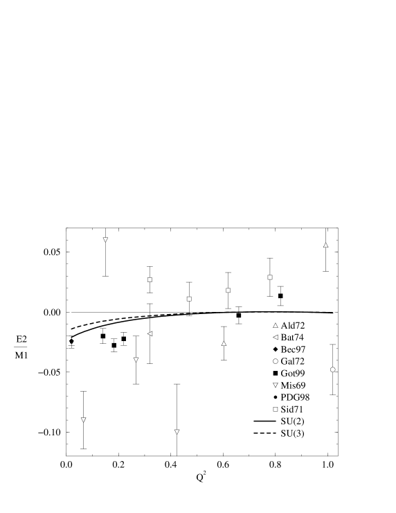
Figure 1: The ratio E2/M1 calculated in the CQSM, in flavor SU(2) and SU(3), for a constituent quark mass of 420 MeV represented as a function of $Q^{2}$ in GeV². Older experimental data (open symbols) is taken from references [1, 2], more recent data (filled symbols) is from [5] and at the photon point from [3].

Figure 2: The ratio C2/M1 calculated in the CQSM, in flavor SU(2) and SU(3), for a constituent quark mass of 420 MeV represented as a function of $Q^{2}$ in GeV². Older experimental data (open symbols) is taken from references [1, 2] and more recent data (filled symbols) is from [4, 5].

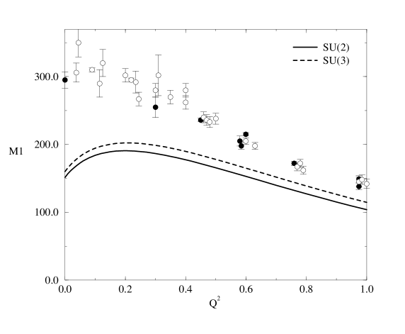
Figure 3: The magnetic dipole amplitude M1${\scriptstyle=-\left[3A_{3/2}+\sqrt{3}A_{1/2}\right]/(2\sqrt{3})}$ calculated in the CQSM, in flavor SU(2) and SU(3), for a constituent quark mass of 420 MeV represented, in units of $10^{-3}$ GeV^-1/2, as a function of $Q^{2}$ (in GeV²). The experimental data is taken from references [2] ($\circ$) and  [34] ($\bullet$).

For the ratio E2/M1, we obtain values, at the photon point, of $-2.1$ % and $-1.4$ %, in SU(2) and SU(3), respectively. A comparison with the most recent photoproduction data [3] in particular with the value $-2.5\pm.5$ %, noted by the Particle Data Group, reveals that our results are smaller, but that the SU(2) value still falls within this estimate. Our prediction for finite momentum transfers yields values which , starting at ${Q^{2}}=0$, tend momotonically to zero and vanish basically for ${Q^{2}}\geq 0.6$ GeV². The predictions are in this range qualitatively in agreement with the data in Ref.[5]. The change to positive E2/M1-values at $Q^{2}=0.8$ GeV² found by Gothe et al. [5] is not reproduced in the present calculations.

For a direct comparison of our numbers with the above data we must take into account that in our formalism the delta is a stable state, which does not decay into nucleon and pion (unless the formalism is developed further which is not done yet). Hence the model allows to calculate the real parts of the transition amplitudes, but not the imaginary ones. Furthermore the extraction of the resonance contribution from the experimental data is not so easely performed and is still a matter of debate. The difficulties are related, among others, to the background contributions originating from the Born term. This question of separating the contributions to the amplitudes has been adressed by several authors [35] and in some cases the non-resonance contributions were found to be large. An unitary ambiguity is known to exist in the case of the E2/M1 ratio [36], related mainly to the models necessary to extract the resonance contribution. A status report concerning the latest determinations of E2/M1 can be found in Ref. [37]. Speed-plot techniques [38] result in E2/M1-ratios of about -3.5%, which are larger than those quoted above.

Concerning the comparison with other models, values for the ratio E2/M1 at the photon point, obtained in the context of electroproduction studies, range from $-0.2$ % in a relativized quark model [7] to $-3.5$ % ($Re$ E2/M1) in the context of heavy baryon chiral perturbation theory [16], passing through $-1.8$ % in the chiral chromodielectric model and $-1.9$ % in the linear sigma model [12], $-2.3$ % in the skyrme model [13] and $-2.4$ % ($Re$ E2/M1) in the chiral bag model [14]. Although the comparison between models may help to understand the physical reasons for the observed ratios, it is also necessary to take into account that different ingredients are involved in the different model calculations above. The models more suitable for a comparison with the CQSM are the constituent quark model and the Skyrme model, between which the CQSM is supposed to interpolate in the limits of small and large soliton sizes, respectively. Indeed, we find that our results in flavour SU(2) at the photon point are between the value of $-0.2$ % [7] for the constituent quark model and the values in the range $-2.6$ % to $-4.9$ % [39] obtained in the Skyrme model. One has also to add however that the nonrelativistic quark model can accomodate higher values, up to $-2$ %, for the ratio E2/M1 [40] if the effects of basis truncation are taken with care. In which regards SU(3), our value $-1.4$ % for E2/M1 at the photon point is smaller than the results for this ratio obtained in hyperon decays within the Skyrme model [41], which fall in the interval $-2.06$ to $-3.14$ % for different model approaches.

It is interesting to note that in subsequent and more refined calculations in these models the results approach an intermediate common value, thus decreasing the difference in the predictions: $-2.3$ % [13] in the Skyrme model and $-3.5$ % [8] for the constituent quark model (in photoproduction). The numerical results obtained in [8] show also the importance of the pionic degrees of freedom, both when compared with previous results in the constituent quark model and with the CQSM and the Skyrme models above, which already include such degrees of freedom from the very beginning, to different extents, though. The role of the meson degrees of freedom may explanain the lower value obtained in SU(3) as compared to SU(2). It may be caused by the poor description of the kaon cloud since the embedding of SU(2) in SU(3) imposes a pion tail for the soliton giving the kaon too large an importance.

For the ratio C2/M1, a comparison made in the same spirit as above for E2/M1, reveals that this ratio slightly underestimates the data above $Q^{2}=0.3$ GeV², where other models [12, 13] obtain a better agreement. Nevertheless, our results are closer to experiment than the quark model results [6, 7]. As for values of $Q^{2}$ between $0$ and $0.3$ GeV², experimentally the situation is not clear. While some old [1] and more recent [4] data seem to show a peaking structure around $0.15$ GeV², more recent results [5] still show a clear decrease of C2/M1 however less pronounced with values similar to those observed for $Q^{2}>0.3$ Gev². As far as we known, no model predicts such a peaking structure. Instead, our results show a smooth growth of the magnitude of the ratio C2/M1 with $Q^{2}$. This behaviour is found within most of the other models in the range of $Q^{2}$ smaller than $1$ GeV² studied. Our results are closer to experimental results, together with  [12, 13], when compared with the remaining models.

6 Summary and Conclusions

The photo- and electroproduction of the $\Delta(1232)$ have been investigated in the chiral quark-soliton model through the computed transition ratios, E2/M1 and C2/M1. The three (four) parameters of the model in SU(2) (SU(3)) were adjusted to the pion decay constant, the pion mass (kaon mass) and from a general fit to nucleon properties. No parametrization adjustment to nucleon-delta transitions was considered. Both ratios E2/M1 as well of C2/M1 are found to be negative for all momentum transfers, as indicated by experiment. The value of E2/M1 at $Q^{2}=0$ underestimates the most recent experimental points by 30 % if one compares the numbers directly. This is the accuracy of the calculations also for finite momentum transfers. Strong fluctuations of C2/M1 at small momentum transfers, as found in some experiments, are not seen in the present approach. Generally the SU(3) calculations do not improve the SU(2) results.

Acknowledgements

The authors thank P. Pobylitsa and M. Polyakov for useful discussions. DU acknowledge the finantial support from PraxisXXI/BD/9300/96 and AS support from PraxisXXI/BD/15681/98 in the final stages of this work. AS and MF acknowledge financial support from Inida Project n432/DAAD. This work was also supported by PRAXIS/PCEX/P/FIS/6/96 (Lisboa) and partially by the DFG (Schwerpunktprogramm) and the COSY-Project Juelich.

Appendix A The Proper-time Regularization

The proper-time regularization is based on the relation, here applied to the real part of the fermionic determinant,

$$\left.-Re\left[Tr\log D(U)\right]+Re\left[Tr\log D(U\!=\!1)\right]\right|_{reg}$$ (72)

$$={1\over 2}{\rm Tr}\int_{0}^{\infty}\frac{du}{u}\phi\left(u,\Lambda\right)\left[e^{-uD^{\dagger}(U)D(U)}-e^{-uD^{\dagger}(1)D(1)}\right]$$

where the arbitrary function $\phi(u,1/\Lambda)$ is chosen as to make the integral finite: it has the form $\theta(u-1/\Lambda^{2})$ in SU(2) and (21) in SU(3).

In order to obtain a finite expression for the sea contribution (48), it is necessary to regularize [28, 29]

$${\rm Tr}\log[D(U)-\epsilon O]={\rm Tr}\log[D(U_{c})+i\Omega-\epsilon O],$$ (73)

in terms of which the functional trace in (48) can be rewritten through

$${\rm Tr}\left[O\langle 0,0|-D^{-1}(U)|0,0\rangle\right]={\delta\over\delta\epsilon(0)}{\rm Tr}\left[D(U)-\epsilon O\right|_{\epsilon=0}.$$ (74)

considering $\epsilon$ real but the operator $O$ not necessarely hermitian.

Since, for the operators considered here, only the real part of ${\rm Tr}\log D_{\epsilon}(U)$ is divergent, it is enough to consider (72). Using

$$e^{\hat{A}+\hat{B}}-e^{\hat{A}} = \int\limits_{0}^{1}d\alpha\>e^{\alpha\hat{A}}\hat{B}e^{(1-\alpha)\hat{B}}$$ (75)

$$+ \int\limits_{0}^{1}d\beta\int\limits_{0}^{1-\beta}d\alpha\>e^{\alpha\hat{A}}\hat{B}e^{\beta\hat{A}}\hat{B}e^{(1-\alpha-\beta)\hat{A}}+\cdots$$

and expanding up to first order in the angular velocity $\Omega$ (37) leads to an expression similar to (49) for the valence part, with ${\cal V}^{(\Omega^{0})}$ and ${\cal V}^{(\Omega^{1})}$ substituted respectively by ${\cal S}^{(\Omega^{0})}$ and ${\cal S}^{(\Omega^{1})}$ given by

$${\cal S}^{(\Omega^{0})}(\mbox{\boldmath$x$})=\sum_{n}{\cal R}_{1}(\varepsilon_{n},\eta)\phi^{\dagger}_{n}(\mbox{\boldmath$x$})\,A^{\dagger}OA\,\phi_{n}(\mbox{\boldmath$x$}),$$ (76)

$${\cal S}^{(\Omega^{1})}(\mbox{\boldmath$x$}) = {1\over 4I_{1}}\sum_{m,n}\Bigl{[}{\cal R}_{2}^{(+)}(\varepsilon_{m},\varepsilon_{n},\eta)J_{a}[\phi^{\dagger}_{m}(\mbox{\boldmath$x$})\,A^{\dagger}OA\,\phi_{n}(\mbox{\boldmath$x$})]$$ (77)

$$\mbox{\hskip 28.45274pt}+{\cal R}_{2}^{(-)}(\varepsilon_{m},\varepsilon_{n},\eta)[\phi^{\dagger}_{m}(\mbox{\boldmath$x$})\,A^{\dagger}OA\,\phi_{n}(\mbox{\boldmath$x$})]J_{a}\Bigr{]}\langle n|\tau_{a}|m\rangle,$$

again in SU(2) for simplicity. The constant $\eta$ is defined by $O^{\dagger}=\eta O$.

The regularization functions appearing in the final expressions for the amplitudes are written in terms of the functions above according to [28, 29]:

$$R_{1}\left(\varepsilon_{n}\right)\equiv R_{1}\left(\varepsilon_{n},-1\right)=-{\varepsilon_{n}\over\sqrt{\pi}}\int_{0}^{\infty}\frac{du}{\sqrt{u}}\phi(u,\Lambda)e^{-u\varepsilon_{n}^{2}}\,,$$ (78)

$$R_{A}\left(\varepsilon_{m},\varepsilon_{n}\right)=-{1\over 2}\left[{\cal R}_{2}^{(+)}(\varepsilon_{m},\varepsilon_{n},-1)+{\cal R}_{2}^{(-)}(\varepsilon_{m},\varepsilon_{n},-1)\right]$$ (79)

$$=-\frac{1}{2\sqrt{\pi}}\int_{0}^{\infty}\frac{du}{\sqrt{u}}\phi(u,\Lambda)\left(\frac{\varepsilon_{n}e^{-u\varepsilon_{n}^{2}}+\varepsilon_{m}e^{-u\varepsilon_{m}^{2}}}{\varepsilon_{m}+\varepsilon_{n}}-\frac{1}{u}\frac{e^{-u\varepsilon_{n}^{2}}-e^{-u\varepsilon_{m}^{2}}}{\varepsilon_{m}^{2}-\varepsilon_{n}^{2}}\right)\,,$$

$$R_{B}\left(\varepsilon_{m},\varepsilon_{n}\right)={1\over 2}\left[{\cal R}_{2}^{(-)}(\varepsilon_{m},\varepsilon_{n},1)-{\cal R}_{2}^{(+)}(\varepsilon_{m},\varepsilon_{n},1)\right]$$ (80)

$$=-\frac{1}{2\pi}\int_{0}^{\infty}\!du\phi(u,\Lambda)\int_{0}^{1}\!d\alpha\frac{\left(1-\alpha\right)\varepsilon_{m}-\alpha\varepsilon_{n}}{\sqrt{\alpha\left(1-\alpha\right)}}\>e^{-u\left[\alpha\varepsilon_{n}^{2}+\left(1-\alpha\right)\varepsilon_{m}^{2}\right]/\Lambda^{2}}\,.$$

References

- [1] J.C. Adler et al., Nucl. Phys. B 46 (1972) 573; K. Bätzner et al., Nucl. Phys. B 76 (1974) 1; R.L. Crawford, Nucl. Phys. B 28 (1971) 573; R. Siddle et al., Nucl. Phys. B 35 (1971) 93.
- [2] S. Galster et al., Phys. Rev. D 5 (1972) 519; C. Mistretta et al., Phys. Rev. 184 (1968) 1487.
- [3] C. Caso et al. (PDG), Eur. Phys. J. C3 (1998) 1; R. Beck et al., Phys. Rev. Lett. 78 (1997) 606; G. Blanpied et al., Phys. Rev. Lett. 79 (1997) 4337.
- [4] F. Kalleicher et al., Z. Phys. A 359 (1997) 201; C. Mertz et al., nucl-ex/9902012; H. Schmieden, Talk given at PANIC99, nucl-ex/9909006.
- [5] R.W. Gothe, Proceedings of the International School of Nuclear Physics, 21st Course: “Electromagnetic Probes and the Structure of Hadrons and Nuclei”, Erice 1999, to be published in Prog. Part. Nucl. Phys. 44.
- [6] M. Bourdeau and N.C. Mukhopadhyay, Phys. Rev. Lett. 58 (1987) 976; S.A. Gogilidze, Yu. Surovtsev anf F.G. Tkebuchava, Yad. Fiz. 45 (1987) 1085; M. Warns, H. Schröder, W. Pfeil and H. Rollnik, Z. Phys. C 45 (1990) 627.
- [7] S. Capstick and G. Karl, Phys. Rev. D 41 (1990) 2767; S. Capstick, Phys. Rev. D 46 (1992) 2864.
- [8] A.J. Buchmann, E. Hernández and A. Faessler, Phys. Rev. C 55 (1997) 448.
- [9] I.G. Aznauryan, Z. Phys. A (1993) 297.
- [10] F. Cardarelli, E. Pace, G. Salmè and S. Simula, Phys. Lett. B 371 (1996) 7.
- [11] M. Aiello, M. Ferraris, M.M Giannini, M. Pizzo and E. Santopinto, Phys. Lett. B 387 (1996) 215.
- [12] M. Fiolhais, B. Golli and S. S̆irca, Phys. Lett. B 373 (1996) 229.
- [13] H. Walliser and G. Holzwarth, Z. Phys. A 357 (1997) 317.
- [14] D.H. Lu, A.W. Thomas and A.G. Williams, Phys. Rev. C 55 (1997) 3108.
- [15] V. Bernard, N. Kaiser, T.S.-H. Lee and Ulf-G. Meissner, Phys. Rep. 246 (1994) 315.
- [16] G.C. Gellas, T.R. Hemmert, C.N. Ktorides and G.I. Poulis, Phys. Rev. D 60 (1999) 54022.
- [17] D. Drechsel, O. Hanstein, S. S. Kamalov and L. Tiator, Nucl. Phys. A 645 (1999) 145.
- [18] D. Diakonov, NORDITA-98-14, hep-ph/9802298.
- [19] Chr.V. Christov, A. Blotz, H.-C. Kim, P. Pobylitsa, T. Watabe, Th. Meissner, E. Ruiz Arriola and K. Goeke, Prog. Part. Nucl. Phys. 37 (1996) 91.
- [20] R. Alkofer, H. Reinhardt and H. Weigel, Phys. Rep. 265 (1996) 139.
- [21] D.I. Diakonov and V.Yu. Petrov, Nucl. Phys. B 272 (1986) 457.
- [22] D.I. Diakonov, V.Yu. Petrov and P.V. Pobylitsa, Nucl. Phys. B 306 (1988) 809.
- [23] Y. Nambu and G. Jona-Lasinio, Phys. Rev. 122 (1961) 354.
- [24] A. Blotz, D. Diakonov, K. Goeke, N.W. Park, V. Petrov and P.V. Pobylitsa, Nucl. Phys. A 555 (1993) 765.
- [25] H. Weigel, R. Alkofer and H. Reinhardt, Nucl. Phys. B 387 (1992) 638.
- [26] A. Blotz, M. Praszałowicz and K. Goeke, Phys. Rev. D 53 (1996) 485.
- [27] H.-C. Kim, A. Blotz, M.V. Polyakov and K. Goeke, Nucl. Phys. A 598 (1996) 379.
- [28] Chr.V. Christov, A.Z. Górski, K. Goeke and P.V. Pobylitsa, Nucl. Phys. A 592 (1995) 513.
- [29] H.-C Kim, A. Blotz, M. Polyakov and K. Goeke, Phys. Rev. D 53 (1996) 4013.
- [30] T. Watabe, Chr. V. Christov and K. Goeke, Phys. Lett. B (1995) 197; T. Watabe and K. Goeke, Proceedings of the Institut for Nuclear Theory- Vol. 4, World Scientific, 1996.
- [31] M. Praszałowicz, T. Watabe and Klaus Goeke, Nucl. Phys. A 647 (1999) 49.
- [32] E. Witten, Nucl. Phys. B223 (1983) 422.
- [33] M. Jaminon, G. Ripka and P. Stassart, Nucl. Phys. A 504 (1989 733.
- [34] W.W. Ash et al., Phys. Lett. B 24 (1967) 154; W. Bartel et al., Phys. Lett. B 28 (1968) 148; S. Stein et al., Phys. Rev. D 12 (1975) 1884.
- [35] R.M. Davidson, N.C. Mukhopadhyay, M.S. Pierce, R.A. Arnt, I.I. Strakovsky and R.L. Workman, Phys. Rev. C 59 (1999) 1059; I.G. Aznauryan, Phys. Rev. D 57 (1998) 2727.
- [36] Th. Wilbois, P. Wilhelm and H. Arenhövel, Phys. Rev. C 57 (1998) 295.
- [37] R.L. Workman, Talk given at Baryons 98, nucl-th/9810013.
- [38] O. Hanstein, D. Drechsel and L. Tiator, Phys. Lett. B 385 (1996) 45.
- [39] A. Wirzba and W. Weise, Phys. Lett. B 188 (1987) 6.
- [40] D. Drechsel and M.M. Giannini, Phys. Lett. B 143 (1984) 329.
- [41] A. Abada, H. Weigel and H. Reinhardt, Phys. Lett. B 366 (1996) 26; T. Haberichter, H.Reinhardt, N.N. Scoccola and H. Weigel, Nucl. Phys. A 615 (1997) 26.