Formation of color-singlet gluon-clusters and inelastic diffractive scattering

Abstract

This is the extensive follow-up report of a recent Letter in which the existence of self-organized criticality (SOC) in systems of interacting soft gluons is proposed, and its consequences for inelastic diffractive scattering processes are discussed. It is pointed out, that color-singlet gluon-clusters can be formed in hadrons as a consequence of SOC in systems of interacting soft gluons, and that the properties of such spatiotemporal complexities can be probed experimentally by examing inelastic diffractive scattering. Theoretical arguments and experimental evidences supporting the proposed picture are presented — together with the result of a systematic analysis of the existing data for inelastic diffractive scattering processes performed at different incident energies, and/or by using different beam-particles. It is shown in particular that the size- and the lifetime-distributions of such gluon-clusters can be directly extracted from the data, and the obtained results exhibit universal power-law behaviors — in accordance with the expected SOC-fingerprints. As further consequences of SOC in systems of interacting soft gluons, the $t$-dependence and the $(M_{x}^{2}/s)$-dependence of the double differential cross-sections for inelastic diffractive scattering off proton-target are discussed. Here $t$ stands for the four-momentum-transfer squared, $M_{x}$ for the missing mass, and $\sqrt{s}$ for the total c.m.s. energy. It is shown, that the space-time properties of the color-singlet gluon-clusters due to SOC, discussed above, lead to simple analytical formulae for $d^{2}\sigma/dt\,d(M_{x}^{2}/s)$ and for $d\sigma/dt$, and that the obtained results are in good agreement with the existing data. Further experiments are suggested.

I Interacting soft gluons in the small-$x_{B}$ region of DIS

A number of striking phenomena have been observed in recent deep-inelastic electron-proton scattering (DIS) experiments in the small-$x_{B}$ region. In particular it is seen, that the contribution of the gluons dominates[1], and that large-rapidity-gap (LRG) events exist[2, 3, 4]. The latter shows that the virtual photons in such processes may encounter “colorless objects” originating from the proton.

The existence of LRG events in these and other[5, 6] scattering processes have attracted much attention, and there has been much discussion [2, 3, 4, 5, 6, 7, 8, 9, 10, 11] on problems associated with the origin and/or the properties of such “colorless objects”. Reactions in which “exchange” of such “colorless objects” dominate are known in the literature [3, 4, 8, 9] as “diffractive scattering processes”. While the concepts and methods used by different authors in describing such processes are in general very much different from one another, all the authors (experimentalists as well as theorists) seem to agree on the following[9] (see also Refs. [References–References, References–References]): (a) Interacting soft gluons play a dominating role in understanding the phenomena in the small-$x_{B}$ region of DIS in general, and in describing the properties of LRG events in particular. (b) Perturbative QCD should be, and can be, used to describe the LRG events associated with high transverse-momentum ($p_{\perp}$) jets which have been observed at HERA[10] and at the Tevatron[7]. Such events are, however, rather rare. For the description of the bulk of LRG events, concepts and methods beyond the perturbative QCD, for example Pomeron Models[8] based on Regge Phenomenology, are needed. It has been suggested a long time ago (see the first two papers in Ref.[References]) that, in the QCD language, “Pomeron-exchange” can be interpreted as “exchange of two or more gluons” and that such results can be obtained by calculating the corresponding Feynman diagrams. It is generally felt that non-perturbative methods should be useful in understanding “the small-$x_{B}$ phenomena”, but the question, whether or how perturbative QCD plays a role in such non-perturbative approaches does not have an unique answer.

In a recent Letter [12], we proposed that the “colorless objects” which play the dominating role in LRG events are color-singlet gluon-clusters due to self-organized criticality, and that optical-geometrical concepts and methods are useful in examing the space-time properties of such objects.

The proposed picture [12] is based on the following observation: In a system of soft gluons whose interactions are not negligible, gluons can be emitted and/or absorbed at any time and everywhere in the system due to color-interactions between the members of the system as well as due to color-interactions of the members with gluons and/or quarks and antiquarks outside the system. In this connection it is important to keep in mind that gluons interact directly with gluons and that the number of gluons in a system is not a conserved quantity. Furthermore, since in systems of interacting soft-gluons the “running-coupling-constant” is in general greater than unity, non-perturbative methods are needed to describe the local interactions associated with such systems. That is, such systems are in general extremely complicated, they are not only too complicated (at least for us) to take the details of local interactions into account (for example by describing the reaction mechanisms in terms of Feynman diagrams), but also too complicated to apply well-known concepts and methods in conventional Equilibrium Statistical Mechanics. In fact, the accumulated empirical facts about LRG events and the basic properties of gluons prescribed by the QCD are forcing us to accept the following picture for such systems:

A system of interacting soft gluons can be, and should be considered as an open, dynamical, complex system with many degrees of freedom, which is in general far from equilibrium.

In our search for an appropriate method to deal with such complex systems, we are led to the following questions: Do we see comparable complex systems in Nature? If yes, what are the characteristic features of such systems, and what can we learn by studying such systems?

II Characteristic features of open dynamical complex systems

Open, dynamical, complex systems which are in general far from equilibrium are not difficult to find in Nature — at least not in the macroscopic world! Such systems have been studied, and in particular the following have been observed by Bak, Tang and Wiesenfeld (BTW) some time ago[13]: This kind of complex systems may evolve to self-organized critical states which lead to fluctuations extending over all length- and time-scales, and that such fluctuations manifest themselves in form of spatial and temporal power-law scaling behaviors showing properties associated with fractal structure and flicker noise, respectively.

To be more precise, BTW[13] and many other authors[14] proposed, and demonstrated by numerical simulations, the following: Open, dynamical, complex systems of locally interacting objects which are in general far from equilibrium can evolve into self-organized structures of states which are barely stable. A local perturbation of a critical state may “propagate”, in the sense that it spreads to (some) nearest neighbors, and than to the next-nearest neighbors, and so on in a “domino effect” over all length scales, the size of such an “avalanche” can be as large as the entire system. Such a “domino effect” eventually terminates after a total time $T$, having reached a final amount of dissipative energy and having effected a total spatial extension $S$. The quantity $S$ is called by BTW the “size”, and the quantity $T$ the “lifetime” of the avalanche — named by BTW a “cluster” (hereafter referred to as BTW-cluster or BTW-avalanche). As we shall see in more details later on, it is of considerable importance to note that a BTW-cluster cannot, and should not be identified with a cluster in the usual sense. It is an avalanche, not a static object with a fixed structure which remains unchanged until it decays after a time-interval (known as the lifetime in the usual sense).

In fact, it has been shown[13, 14] that the distribution ($D_{S}$) of the “size” (which is a measure of the dissipative energy, $S$) and the distribution ($D_{T}$) of the lifetime ($T$) of BTW-clusters in such open, dynamical, complex systems obey power-laws:

$$D_{S}(S)\sim S^{-\mu},$$ (1)

$$D_{T}(T)\sim T^{-\nu},$$ (2)

where $\mu$ and $\nu$ are positive real constants. Such spatial and temporal power-law scaling behaviors can be, and have been, considered as the universal signals — the “fingerprints” — of the locally perturbed self-organized critical states in such systems. It is expected[13, 14] that the general concept of self-organized criticality (SOC), which is complementary to chaos, may be the underlying concept for temporal and spatial scaling in a wide class of open, non-equilibrium, complex systems — although it is not yet known how the exponents of such power laws can be calculated analytically from fundamental theories such that for gravitation or that for electromagnetism.

SOC has been observed experimentally in a large number of open, dynamical, complex systems in non-equilibrium[13, 14, 15, 16, 17, 18] among which the following examples are of particular interest, because they illuminate several aspects of SOC which are relevant for the discussion in this paper.

First, the well-known Gutenberg-Richter law[19, 15] for earthquakes as a special case of Eq.(1): In this case, earthquakes are BTW-clusters due to SOC. Here, $S$ stands for the released energy (the magnitude) of the observed earthquakes. $D_{S}(S)$ is the number of earthquakes at which an energy $S$ is released. Such a simple law is known to be valid for all earthquakes, large (up to $8$ or $9$ in Richter scale) or small! We note, the power-law behavior given by the Gutenberg-Richter law implies in particular the following. The question “How large is a typical earthquake?” does not make sense!

Second, the sandpile experiments[13, 14] which show the simple regularities mentioned in Eqs.(1) and (2): In this example, we see how local perturbation can be caused by the addition of one grain of sand (note that we are dealing with an open system!). Here, we can also see how the propagation of perturbation in form of “domino effect” takes place, and develops into BTW-clusters/avalanches of all possible sizes and durations. The size- and duration-distributions are given by Eqs.(1) and (2), respectively. This example is indeed a very attractive one, not only because such experiments can be, and have been performed in laboratories [14], but also because they can be readily simulated on a PC[13, 14].

Furthermore, it has been pointed out, and demonstrated by simple models[14, 16, 17, 18], that the concept of SOC can also be applied to Biological Sciences. It is amazing to see how phenomena as complicated as Life and Evolution can be simulated by simple models such as the “Game of Life”[16] and the “Evolution Model”[17, 18].

Having seen that systems of interacting soft-gluons are open, dynamical, complex systems, and that a wide class of open, dynamical, complex systems in the macroscopic world evolve into self-organized critical states which lead to fluctuations extending over all length- and time-scales, it seems natural to ask the following: Can such states and such fluctuations also exist in the microscopic world — on the level of quarks and gluons? In particular: Can SOC be the dynamical origin of color-singlet gluon-clusters which play the dominating role in inelastic diffractive scattering processes?

III SOC in inelastic diffractive scattering processes?

One of the main goals of the present paper is to answer the questions mentioned at the end of the last section. We discuss in this and in the following four sections, how to look for signals of SOC in systems of interacting gluons, and what can we see when we look for signals of SOC in scattering processes in which systems of interacting gluons play the dominating role.

Here, we explicitly see: (a) The fundamental properties of the gluons, (b) the necessary conditions for the occurrence of SOC, and (c) the available technical possibilities strongly suggest that the most favorable place to study the possible existence of such signals is (i) to look at the experimental results obtained in events associated with large rapidity gaps in deep-inelastic scattering, (ii) to look at the experimental results in inelastic diffractive hadron-hadron scattering, and (iii) to compare such observations with each other.

Having the special role played by “the colorless objects” in inelastic diffractive scattering in mind, let us begin our discussion with the question: What are such “colorless objects”? Up to now, we do not know much about such objects. We know that they carry neither color- nor any flavor-quantum numbers. We know that they exist in high-energy reactions where soft gluons play the dominating role. We know that they can be probed in diffractive scattering processes, in the sense that they can interact with different beam-particles. But, there are a lot more which we do not know, for example: What is the mass of a typical “colorless object”? What is the lifetime of a typical “colorless object”? Do such objects have distinct electromagnetic structures? Are they hadron-like? Before more and better empirical facts about such objects become available, guesses and/or speculations may be helpful, provided that they agree with the existing data, and they are consistent with the fundamental theoretical knowledge — in particular consistent with the basic properties of the gluons (the direct gluon-gluon coupling prescribed by the QCD-Lagrangian, the confinement, and the non-conservation of gluon number, etc.). In this sense, we may wish to ask: Is it possible that the colorless objects are BTW-clusters which exist due to SOC in systems of interacting soft gluons? We are aware of the fact that the existence of SOC cannot (at least cannot yet) be derived from a basic theory such as QCD [Perhaps this can be and/or should be compared with the fact that the Gutenberg Richter law for earthquakes cannot (at least cannot yet) be derived from gravitational theory]. But, as in the case of earthquakes or any other open dynamical systems which leads to SOC, we can and we should ask: Can this be checked experimentally? Can this be done by looking for characteristic properties of SOC — in particular the SOC-fingerprints mentioned in Eqs.(1) and (2) in the relevant experiments?

To answer these questions, it is useful to recall the following: Since the “colorless objects” are color-singlets which can exist inside and/or outside the proton, the interactions between such color-singlets as well as those between such objects and “the mother proton” should be of Van der Waals type. Hence, it is expected that such a colorless object can be readily separated as an entire object from the mother proton in scattering processes in which the momentum-transfer is sufficient to overcome the binding energy due to the Van der Waals type of interactions. This means, in inelastic diffractive scattering the beam-particle (which is the virtual photon $\gamma^{\star}$ in DIS) should have a chance to encounter one of the color-singlet gluon-clusters. For the reasons mentioned above, the struck colorless object can simply be “knocked out” and/or “carried away” by the beam-particle in such a collision event. Hence, it seems that the question whether “the colorless objects” are indeed BTW-clusters is something that can be answered experimentally. In this connection we recall that, according to the general theory of SOC[13, 14], the size of a BTW-cluster is characterized by its dissipative energy, and in case of systems of interacting soft gluons associated with the proton, the dissipative energy carried by the BTW-cluster should be proportional to the energy fraction ($x_{P}$) carried by the colorless object. Hence, if the colorless object can indeed be considered as a BTW-cluster due to SOC, we should be able to obtain information about the size-distribution of such color-singlet gluon-clusters by examing the $x_{P}$-distributions of LRG events in the small-$x_{B}$ region of DIS.

Having this in mind, we now take a closer look at the measured [3] “diffractive structure function” $F_{2}^{D(3)}(\beta,Q^{2};x_{P})\equiv\int dtF_{2}^{D(4)}(\beta,Q^{2};x_{P},t)$. Here, we note that $F_{2}^{D(4)}(\beta,Q^{2};x_{P},t)$ is related [3, 4, 8, 9, 10] to the differential cross-section for large-rapidity-gap events

$${d^{4}\sigma^{D}\over d\beta dQ^{2}dx_{P}dt}={4\pi\alpha^{2}\over\beta Q^{4}}(1-y+{y^{2}\over 2})F_{2}^{D(4)}(\beta,Q^{2};x_{P},t),$$ (3)

in analogy to the relationship between the corresponding quantities [namely $d^{2}\sigma/(dx_{B}\,dQ^{2})$ and $F_{2}(x_{B},Q^{2})$] for normal deep-inelastic electron-proton scattering events

$${d^{2}\sigma\over dx_{B}dQ^{2}}={4\pi\alpha^{2}\over x_{B}Q^{4}}(1-y+{y^{2}\over 2})F_{2}(x_{B},Q^{2}).$$ (4)

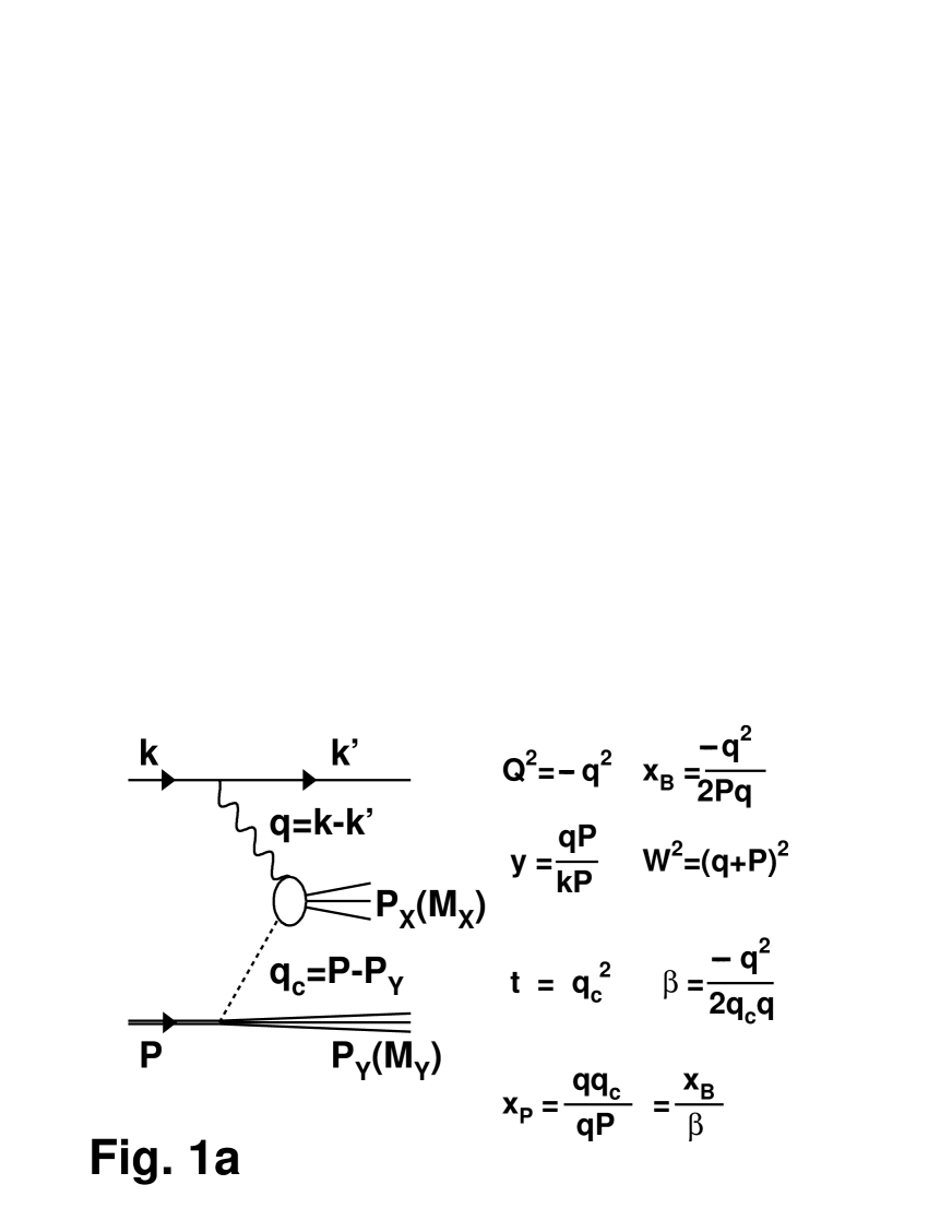
Figure 1: The well-known Feynman diagrams (a) for diffractive and (b) for normal deep-inelastic electron-proton scattering are shown together with the relevant kinematical variables which describe such processes.

The kinematical variables, in particular $\beta$, $Q^{2}$, $x_{P}$ and $x_{B}$ (in both cases) are directly measurable quantities, the definitions of which are shown in Fig.1 together with the corresponding diagrams of the scattering processes. We note that, although these variables are Lorentz-invariants, it is sometimes convenient to interpret them in a “fast moving frame”, for example the electron-proton center-of-mass frame where the proton’s 3-momentum $\vec{P}$ is large (i.e. its magnitude $|\vec{P}|$ and thus the energy $P^{0}\equiv(|\vec{P}|^{2}+M^{2})^{1/2}$ is much larger than the proton mass $M$). While $Q^{2}$ characterizes the virtuality of the space-like photon $\gamma^{\star}$, $x_{B}$ can be interpreted, in such a “fast moving frame” (in the framework of the celebrated parton model), as the fraction of proton’s energy $P^{0}$ (or longitudinal momentum $|\vec{P}|$) carried by the struck charged constituent.

We recall, in the framework of the parton model, $F_{2}(x_{B},$ $Q^{2})/x_{B}$ for “normal events” can be interpreted as the sum of the probability densities for the above-mentioned $\gamma^{\star}$ to interact with a charged constituent of the proton. In analogy to this, the quantity $F_{2}^{D(3)}(\beta,Q^{2};x_{P})/\beta$ for LRG events can be interpreted as the sum of the probability densities for $\gamma^{\star}$ to interact with a charged constituent which carries a fraction $\beta\equiv x_{B}/x_{P}$ of the energy (or longitudinal momentum) of the colorless object, under the condition that the colorless object (which we associate with a system of interacting soft gluons) carries a fraction $x_{P}$ of proton’s energy (or longitudinal momentum). We hereafter denote this charged-neutral and color-neutral gluon-system by $c^{\star}_{0}$ (in Regge pole models[8] this object is known as the “Pomeron”). Hence, by comparing Eq.(3) with Eq.(4) and by comparing the two diagrams shown in Fig.1a and Fig.1b, it is tempting to draw the following conclusions:

The diffractive process is nothing else but a process in which the virtual photon $\gamma^{\star}$ encounters a $c_{0}^{\star}$, and $\beta$ is nothing else but the Bjorken-variable with respect to $c_{0}^{\star}$ (this is why it is called $x_{BC}$ in Ref.[References]). This means, a diffractive $e^{-}p$ scattering event can be envisaged as an event in which the virtual photon $\gamma^{\star}$ collides with “a $c_{0}^{\star}$-target” instead of “the proton-target”. Furthermore, since $c_{0}^{\star}$ is charge-neutral, and a photon can only directly interact with an object which has electric charges and/or magnetic moments, it is tempting to assign $c_{0}^{\star}$ an electromagnetic structure function $F_{2}^{c}(\beta,Q^{2})$, and study the interactions between the virtual photon and the quark(s) and antiquark(s) inside $c_{0}^{\star}$. In such a picture (which should be formally the same as that of Regge pole models[8], if we would replace the $c_{0}^{\star}$’s by “pomerons”) we are confronted with the following two questions:

First, is it possible and meaningful to discuss the $x_{P}$-distributions of the $c_{0}^{\star}$’s without knowing the intrinsic properties, in particular the electromagnetic structures, of such objects?

Second, are the $c_{0}^{\star}$’s hadron-like, such that the electromagnetic structure of a (a typical, or an average) $c_{0}^{\star}$ can be studied in the same way as those for ordinary hadron?

Since we wish to begin the quantitative discussion with something familiar to most of the readers in this community, and we wish to differentiate between the conventional-approach and the SOC-approach, we would like to discuss the second question here, and leave the first question to the next section. We recall (see in particular the last two papers in Ref.[References]), in order to see whether the second question can be answered in the affirmative, we need to know whether $F_{2}^{D(3)}(\beta,Q^{2};x_{P})$ can be factorized in the form

$$F_{2}^{D(3)}(\beta,Q^{2};x_{P})=f_{c}(x_{P})F_{2}^{c}(\beta,Q^{2}).$$ (5)

Here, $f_{c}(x_{P})$ plays the role of a “kinematical factor” associated with the “target $c_{0}^{\star}$”, and $x_{P}$ is the fraction of proton’s energy (or longitudinal momentum) carried by $c_{0}^{\star}$. [We could call $f_{c}(x_{P})$ “the $c_{0}^{\star}$-flux” — in exactly the same manner as in Regge pole models[8], where it is called “the pomeron flux”.] $F_{2}^{c}(\beta,Q^{2})$ is “the electromagnetic structure function of $c_{0}^{\star}$” [the counterpart of $F_{2}(x_{B},Q^{2})$ of the proton] which — in analogy to proton (or any other hadron) — can be expressed as

$$\frac{F_{2}^{c}(\beta,Q^{2})}{\beta}=\sum_{i}e_{i}^{2}[q_{i}^{c}(\beta,Q^{2})+\bar{q}_{i}^{c}(\beta,Q^{2})],$$ (6)

where $q_{i}^{c}(\bar{q}_{i}^{c})$ stands for the probability density for $\gamma^{\star}$ to interact with a quark (antiquark) of flavor $i$ and electric charge $e_{i}$ which carries a fraction $\beta$ of the energy (or longitudinal momentum) of $c_{0}^{\star}$. It is clear that Eq.(6) should be valid for all $x_{P}$-values in this kinematical region, that is, both the right- and the left-hand-side of Eq.(6) should be independent of the energy (momentum) carried by the “hadron” $c_{0}^{\star}$.

Hence, to find out experimentally whether the second question can be answered in the affirmative, we only need to check whether the data are in agreement with the assumption that $F_{2}^{c}(\beta,Q^{2})$ prescribed by Eqs.(5) and (6) exists. For such a test, we take the existing data[3] and plot $\log[F_{2}^{D(3)}(\beta,Q^{2};x_{P})/\beta]$ against $\log\beta$ for different $x_{P}$-values. We note, under the assumption that the factorization shown in Eq.(5) is valid, the $\beta$-dependence for a given $Q^{2}$ in such a plot should have exactly the same form as that in the corresponding $\log[F_{2}^{c}(\beta,Q^{2})/\beta]$ vs $\log\beta$ plot; and that the latter is the analog of $\log[F_{2}(x_{B},Q^{2})/x_{B}]$ vs $\log x_{B}$ plot for normal events. In Fig.2 we show the result of such plots for three fixed $Q^{2}$-values (3.5, 20 and 65 GeV², as representatives of three different ranges in $Q^{2}$). Our goal is to examine whether or how the $\beta$-dependence of the function given in Eq.(6) changes with $x_{P}$. In principle, if there were enough data points, we should, and we could, do such a plot for the data-sets associated with every $x_{P}$-value. But, unfortunately there are not so much data at present. What we can do, however, is to consider the $\beta$-distributions in different $x_{P}$-bins, and to vary the bin-size of $x_{P}$, so that we can explicitly see whether/how the shapes of the $\beta$-distributions change. The results are shown in Fig.2. The $\beta$-distribution in the first row, corresponds to the integrated value $\tilde{F}^{D}_{2}(\beta,Q^{2})$ shown in the literature[3, 9]. Those in the second and in the third row are obtained by considering different bins and/or by varying the sizes of the bins. By joining the points associated with a given $x_{P}$-interval in a plot for a given $Q^{2}$, we obtain the $\beta$-distribution for a $c_{0}^{\star}$ carrying approximately the amount of energy $x_{P}P^{0}$, encountered by a photon of virtuality $Q^{2}$. Taken together with Eq.(6) we can then extract the distributions $q_{i}^{c}(\beta,Q^{2})$ and $\bar{q}_{i}^{c}(\beta,Q^{2})$ for this $Q^{2}$-value, provided that $F_{2}^{c}(\beta,Q^{2})/\beta$ is independent of $x_{P}$. But, as we can see in Fig.2, the existing data[3] show that the $x_{P}$-dependence of this function is far from being negligible! Note in particular that according to Eq.(5), by choosing a suitable $f_{P}(x_{P})$ we can shift the curves for different $x_{P}$-values in the vertical direction (in this log-log plot); but we can never change the shapes of the $\beta$-distributions which are different for different $x_{P}$-values!

In order to see, and to realize, the meaning of the $x_{P}$-dependence of the distributions of the charged constituents of $c^{\star}_{0}$ expressed in terms of $F_{2}^{c}(\beta,Q^{2})/\beta$ in LRG events [see Eqs.(5) and (6)], let us, for a moment, consider normal deep-inelastic scattering events in the $x_{B}$-region where quarks dominate ($x_{B}>0.1$, say). Here we can plot the data for $\log[F_{2}(x_{B},Q^{2})/x_{B}]$ as a function of $\log x_{B}$ obtained at different incident energies ($P^{0}$’s) of the proton. Suppose we see, that at a given $Q^{2}$, the data for $x_{B}$-distributions taken at different values of $P^{0}$ are very much different. Would it still be possible to introduce $F_{2}(x_{B},Q^{2})$ as “the electromagnetic structure function” of the proton, from which we can extract the $x_{B}$-distribution of the quarks $q_{i}(x_{B},Q^{2})$ at a given $Q^{2}$? The fact that it is not possible to assign an $x_{P}$-independent structure function $F_{2}^{c}(\beta,Q^{2})/\beta$ to $c_{0}^{\star}$ which stands for the “Pomeron”, and whose “flux” $f_{c}(x_{P})$ is expected to be independent of $\beta$ and $Q^{2}$, deserves to be taken seriously. It strongly suggests that the following picture cannot be true: “There exists an universal colorless object (call it Pomeron or $c_{0}^{\star}$ or something else) the exchange of which describes diffractive scattering in general and DIS off proton in particular. This object is hadron-like in the sense that it has not only a typical size and a typical lifetime, but also a typical electromagnetic structure which can e.g. be measured and described by an electromagnetic structure function”.

In summary of this section, we note that the empirical facts mentioned above show that no energy-independent electromagnetic structure function can be assigned to the expected universal colorless object $c_{0}^{\star}$. This experimental fact is of considerable importance, because it is the first indication that, if there is an universal “colorless object”, this object cannot be considered as an ordinary hadron. It has to be something else! In fact, as we shall see below, this property is closely related to the observation that such an object cannot have a typical size, or a typical lifetime. To be more precise, the fact that the data [3] cannot accommodate the simple factorization assumption shown in Eq.(5), in which a universal Pomeron flux with a unique hadron-like Pomeron structure function exists, can be considered as further support to the proposed SOC picture because a BTW-cluster, which has neither a typical size nor a typical lifetime, cannot have an universal static structure. With these characteristic properties of the colorless objects in mind, we see [20] an overlap between the SOC-picture and the partonic picture for Pomeron and/or Pomeron and Reggeon [8, 20] in which, beside the Pomeron, exchange of ( in general infinite number of) subleading trajectories are possible. In fact, it has been reported [3, 4] that very good agreement can be achieved between the data [3, 4] and these types of models. Hence, in order to differentiate between the two approaches, it is not only useful but also necessary to examine the corresponding predictions for the dependence on the invariant momentum transfer $t$. This will be discussed in detail in Sections VIII - XI.

IV Distributions of the gluon-clusters

After having seen that the existing data does not allow us to assign an energy-independent electromagnetic structure function to “the colorless object” such that the universal colorless object ($c_{0}^{\star}$) can be treated as an ordinary hadron, let us now come back to the first question in Section III, and try to find out whether it is never-the-less possible, and meaningful, to talk about the $x_{P}$-distribution of $c_{0}^{\star}$. As we shall see in this section, the answer to this question is Yes! Furthermore, we shall also see, in order to answer this question in the affirmative, we do not need the factorization mentioned in Eq.(5), and we do not need to know whether the $c_{0}^{\star}$’s are hadron-like. But, as we have already mentioned above, it is of considerable importance to discuss the second question so that we can understand the origin and the nature of the $c_{0}^{\star}$’s.

In view of the fact that we do use the concept “distributions of gluons” in deep-inelastic lepton-hadron scattering, although the gluons do not directly interact with the virtual photons, we shall try to introduce the notion “distribution of $c_{0}^{\star}$” in a similar manner. In order to see what we should do for the introduction of such distributions, let us recall the following:

For normal deep-inelastic $e^{-}p$ collision events, the structure function $F_{2}(x_{B},Q^{2})$ can be expressed in terms of the distributions of partons, where the partons are not only quarks and antiquarks, but also gluons which can contribute to the structure function by quark-antiquark pair creation and annihilation. In fact, in order to satisfy energy-momentum-conservation (in the electron-proton system), the contribution of the gluons $x_{g}g(x_{g},Q^{2})$ has to be taken into account in the energy-momentum sum rule for all measured $Q^{2}$-values. Here, we denote by $g(x_{g},Q^{2})$ the probability density for the virtual photon $\gamma^{\star}$ (with virtuality $Q^{2}$) to meet a gluon which carries the energy (momentum) fraction $x_{g}$ of the proton, analogous to $q_{i}(x_{B},Q^{2})$ [or $\bar{q}_{i}(x_{B},Q^{2})$] which stands for the probability density for this $\gamma^{\star}$ to interact with a quark (or an antiquark) of flavor $i$ and electric charge $e_{i}$ which carries the energy (momentum) fraction $x_{B}$ of the proton. We note, while both $x_{B}$ and $x_{g}$ stand for energy (or longitudinal momentum) fractions carried by partons, the former can be, but the latter cannot be directly measured.

Having these, in particular the energy-momentum sum rule in mind, we immediately see the following: In a given kinematical region in which the contributions of only one category of partons (for example quarks for $x_{B}>0.1$ or gluons for $x_{B}<10^{-2}$) dominate, the structure function $F_{2}(x_{B},Q^{2})$ can approximately be related to the distributions of that particular kind of partons in a very simply manner. In fact, the expressions below can be, and have been, interpreted as the probability-densities for the virtual photon $\gamma^{\star}$ (with virtuality $Q^{2}$) to meet a quark or a gluon which carries the energy (momentum) fraction $x_{B}$ or $x_{g}$ respectively.

$${F_{2}(x_{B},Q^{2})\over x_{B}} \approx \sum_{i}e_{i}^{2}\,q_{i}(x_{B},Q^{2})\mbox{\hskip 28.45274ptor\hskip 28.45274pt}$$

$${F_{2}(x_{B},Q^{2})\over x_{g}} \approx g(x_{g},Q^{2})\mbox{\ .}$$ (7)

The relationship between $q_{i}(x_{B},Q^{2})$, $g(x_{g},Q^{2})$ and $F_{2}(x_{B},Q^{2})$ as they stand in Eq.(IV) are general and formal (this is the case especially for that between $g$ and $F_{2}$) in the following sense: Both $q_{i}(x_{B},Q^{2})$ and $g(x_{g},Q^{2})$ contribute to the energy-momentum sum rule and both of them are in accordance with the assumption that partons of a given category (quarks or gluons) dominate a given kinematical region (here $x_{B}>0.1$ and $x_{B}<10^{-2}$, respectively). But, neither the dynamics which leads to the observed $Q^{2}$-dependence nor the relationship between $x_{g}$ and $x_{B}$ are given. This means, without further theoretical inputs, the simple expression for $g(x_{g},Q^{2})$ as given by Eq.(IV) is practically useless!

Having learned this, we now discuss what happens if we assume, in diffractive lepton-nucleon scattering, that the color-singlet gluon-clusters ($c_{0}^{\star}$’s) dominate the small-$x_{B}$ region ($x_{B}<10^{-2}$, say). In this simple picture, we are assuming that the following is approximately true: The gluons in this region appear predominantly in form of $c_{0}^{\star}$’s. The interaction between the struck $c_{0}^{\star}$ and the rest of the proton can be neglected during the $\gamma$-$c_{0}^{\star}$ collision such that we can apply impulse-approximation to the $c_{0}^{\star}$’s in this kinematical region. That is, here we can introduce — in the same manner as we do for other partons (see Eq.(IV)), a probability density $D_{S}(x_{P}|\beta,Q^{2})$ for $\gamma^{\star}$ in the diffractive scattering process to “meet” a $c_{0}^{\star}$ which carries the fraction $x_{P}$ of the proton’s energy $P^{0}=(|\vec{P}|^{2}+M^{2})^{1/2}\approx|\vec{P}|$ (where $\vec{P}$ is the momentum and $M$ is the mass of the proton). In other words, in diffractive scattering events for processes in the kinematical region $x_{B}<10^{-2}$, we should have, instead of $g(x_{g},Q^{2})$, the following:

$${F_{2}^{D(3)}(\beta,Q^{2};x_{P})\over x_{P}}\approx D_{S}(x_{P}|\beta,Q^{2})\,.$$ (8)

Here, $x_{P}P^{0}$ is the energy carried by $c_{0}^{\star}$, and $\beta$ indicates the corresponding fraction carried by the struck charged constituent in $c_{0}^{\star}$. In connection with the similarities and the differences between $q_{i}(x_{B},Q^{2})$, $g(x_{B},Q^{2})$ in Eq.(IV) and $D_{S}(x_{P}|\beta,Q^{2})$ in Eq.(8), it is useful to note in particular the significant difference between $x_{g}$ and $x_{P}$, and thus that between the $x_{g}$-distribution $g(x_{g},Q^{2})$ of the gluons and the $x_{P}$-distribution $D_{S}(x_{P}|\beta,Q^{2})$ of the $c^{\star}_{0}$’s: Both $x_{g}$ and $x_{P}$ are energy (longitudinal momentum) fractions of charge-neutral objects, with which $\gamma^{\star}$ cannot directly interact. But, in contrast to $x_{g}$, $x_{P}$ can be directly measured in experiments, namely by making use of the kinematical relation

$$x_{P}\approx{Q^{2}+M_{x}^{2}\over Q^{2}+W^{2}},$$ (9)

and by measuring the quantities $Q^{2}$, $M_{x}^{2}$ and $W^{2}$ in every collision event. Here, $Q$, $M_{x}$ and $W$ stand respectively for the invariant momentum-transfer from the incident electron, the invariant-mass of the final hadronic state after the $\gamma^{\star}-c_{0}^{\star}$ collision, and the invariant mass of the entire hadronic system in the collision between $\gamma^{\star}$ and the proton. Note that $x_{B}\equiv\beta x_{P}$, hence $\beta$ is also measurable. This means, in sharp contrast to $g(x_{g},Q^{2})$, experimental information on $D_{S}(x_{P}|\beta,Q^{2})$ in particular its $x_{P}$-dependence can be obtained — without further theoretical inputs!

V The first SOC-fingerprint: Spatial scaling

We mentioned at the beginning of Section III, that in order to find out whether the concept of SOC indeed plays a role in diffractive DIS we need to check the fingerprints of SOC shown in Section II, and that such tests can be made by examing the corresponding cluster-distributions obtained from experimental data. We are now ready to do this, because we have learned in Sections III and IV, that it is not only meaningful but also possible to extract $x_{P}$-distributions from the measured diffractive structure functions, although the $c_{0}^{\star}$’s cannot be treated as hadrons. In fact, as we can explicitly see in Eqs.(8) and (9), in order to extract the $x_{P}$-dependence of the $c_{0}^{\star}$’s from the data, detailed knowledge about the intrinsic structure of the $c_{0}^{\star}$’s are not necessary.

Having these in mind, we now consider $D_{S}$ as a function of $x_{P}$ for given values of $\beta$ and $Q^{2}$, and plot $F_{2}^{D(3)}(\beta,Q^{2};x_{P})/x_{P}$ against $x_{P}$ for different sets of $\beta$ and $Q^{2}$. The results of such log-log plots are shown in Fig.3. As we can see, the data[3, 4] suggest that the probability-density for the virtual photon $\gamma^{\star}$ to meet a color-neutral and charged-neutral object $c_{0}^{\star}$ with energy (longitudinal momentum) fraction $x_{P}$ has a power-law behavior in $x_{P}$, and the exponent of this power-law depends very little on $Q^{2}$ and $\beta$. This is to be compared with $D_{S}(S)$ in Eq.( 1), where $S$, the dissipative energy (the size of the BTW-cluster) corresponds to the energy of the system $c_{0}^{\star}$. The latter is $x_{P}P^{0}$, where $P^{0}$ is the total energy of the proton.

It means, the existing data[3, 4] show that $D_{S}(x_{P}|\beta,Q^{2})$ exhibits the same kind of power-law behavior as the size-distribution of BTW-clusters. This result is in accordance with the expectation that self-organized critical phenomena may exist in systems of interacting soft gluons in diffractive deep-inelastic electron-proton scattering processes.

We note, up to now, we have only argued (in Section I) that such gluon-systems are open, dynamical, complex systems in which SOC may occur, and we have mentioned (in Section II) the ubiquitousness of SOC in Nature. Having seen the experimental evidence that one of the “SOC-fingerprints” (which are necessary conditions for the existence of SOC) indeed exists, let us now take a second look at such gluon-systems from a theoretical standpoint. Viewed from a “fast moving frame” which can for example be the electron-proton c.m.s. frame, such systems of interacting soft gluons are part of the proton (although color-singlets can also be outside the confinement region). Soft gluons can be intermittently emitted or absorbed by gluons in such a system, as well as by gluons, quarks and antiquarks outside the system. The emission- and absorption-processes are due to local interactions prescribed by the well-known QCD-Lagrangian (here “the running coupling constants” are in general large, because the distances between the interacting colored objects cannot be considered as “short”; remember that the spatial dimension of a $c_{0}^{\star}$ can be much larger than that of a hadron!). In this connection, it is useful to keep the following in mind: Due to the complexity of the system, details about the local interactions may be relatively unimportant, while general and/or global features — for example energy-flow between different parts (neighbors and neighbor’s neighbors $\ldots$) of the system — may play an important role.

How far can one go in neglecting dynamical details when one deals with such open complex systems? In order to see this, let us recall how Bak and Sneppen[17] succeeded in modeling some of the essential aspects of The Evolution in Nature. They consider the “fitness” of different “species”, related to one another through a “food chain”, and assumed that the species with the lowest fitness is most likely to disappear or mutate at the next time-step in their computer simulations. The crucial step in their simulations that drives evolution is the adaption of the individual species to its present environment (neighborhood) through mutation and selection of a fitter variant. Other interacting species form part of the environment. This means, the neighbors will be influenced by every time-step. The result these authors obtained strongly suggests that the process of evolution is a self-organized critical phenomenon. One of the essential simplifications they made in their evolution models[17, 18] is the following: Instead of the explicit connection between the fitness and the configuration of the genetic codes, they use random numbers for the fitness of the species. Furthermore, as they have pointed out in their papers, they could in principle have chosen to model evolution on a less coarse-grained scale by considering mutations at the individual level rather than on the level of species, but that would make the computation prohibitively difficult.

Having these in mind, we are naturally led to the questions: Can we consider the creation and annihilation processes of colorless systems of interacting soft gluons associated with a proton as “evolution” in a microscopic world? Before we try to build models for a quantitative description of the data, can we simply apply the existing evolution models[17, 18] to such open, dynamical, complex systems of interacting soft gluons, and check whether some of the essential features of such systems can be reproduced?

To answer these questions, we now report on the result of our first trial in this direction: Based on the fact that we know very little about the detailed reaction mechanisms in such gluon-systems and practically nothing about their structures, we simply ignore them, and assume that they are self-similar in space (this means, color-singlet gluon-clusters ($c_{0}^{\star}$) can be considered as clusters of $c_{0}^{\star}$’s and so on). Next, we divide them into an arbitrary given number of subsystems $s_{i}$ (which may or may not have the same size). Such a system is open, in the sense that neither its energy $\varepsilon_{i}$, nor its gluon-number $n_{i}$ has a fixed value. Since we do not know, in particular, how large the $\varepsilon_{i}$’s are, we use random numbers. As far as the $n_{i}$’s are concerned, since we do not know how these numbers are associated with the energies in the subsystems $s_{i}$, except that they are not conserved quantities, we just ignore them, and consider only the $\varepsilon_{i}$’s. As in Ref.[References] or in Ref.[References], the random number of this subsystem as well as those of the fixed[17] or random (see the first paper of Ref.[References]) neighbors will be changed at every time-step. Note, this is how we simulate the processes of energy flow due to exchange of gluons between the subsystems, as well as those with gluons/quarks/antiquarks outside the system. In other words, in the spirit of Bak and Sneppen[17] we are neglecting the dynamical details totally. Having in mind that, in such systems, the gluons as well as the subsystems ($s_{i}$’s) of gluons are virtual (space-like), we can ask: “How long can such a colorless subsystem $s_{i}$ of interacting soft gluons exist, which carries energy $\varepsilon_{i}$?” According to the uncertainty principle, the answer should be: “The time interval in which the subsystem $s_{i}$ can exist is proportional to $1/\varepsilon_{i}$, and this quantity can be considered as the lifetime $\tau_{i}$ of $s_{i}$.” In this sense, those colorless subsystems of gluons are expected to have larger probabilities to mutate when they are associated with higher energies, and thus shorter “lifetimes”. Note that the basic local interaction in this self-organized evolution process is the emission (or absorption) of gluons by gluons prescribed by the QCD-Lagrangian — although the detailed mechanisms (which can in principle be explicitly written down by using the QCD-Lagrangian) do not play a significant role.

In terms of the evolution model[17, 18] we now call $s_{i}$ the “species” and identify the corresponding lifetime $\tau_{i}$ as the “fitness of $s_{i}$”. Because of the one-to-one correspondence between $\tau_{i}$ and $\varepsilon_{i}$, where the latter is a random number, we can also directly assign random numbers to the $\tau_{i}$’s instead. From now we can adopt the evolution model[17, 18] and note that, at the start of such a process (a simulation), the fitness on average grow, because the least fit are always eliminated. Eventually the fitness do not grow any further on average. All gluons have a fitness above some threshold. At the next step, the least fit species (i.e. the most energetic subsystem $s_{i}$ of interacting soft gluons), which would be right at the threshold, will be “replaced” and starts an avalanche (or punctuation of mutation events), which is causally connected with this triggering “replacement”. After a while, the avalanche will stop, when all the fitnesses again will be over that threshold. In this sense, the evolution goes on, and on, and on. As in Refs.[References] and [References], we can monitor the duration of every avalanche, that is the total number of mutation events in everyone of them, and count how many avalanches of each size are observed. The avalanches mentioned here are special cases of those discussed in Section II. Their size- and lifetime-distributions are given by Eq.(1) and Eq.(2), respectively. Note in particular that the avalanches in the Bak-Sneppen model correspond to sets of subsystems $s_{i}$, the energies ($\epsilon_{i}$) of which are too high “to be fit for the colorless systems of low-energy gluons”. It means, in the proposed picture, what the virtual photon in deep-inelastic electron-proton scattering “meet” are those “less fit” one — those who carry “too much” energy. In a geometrical picture this means, it is more probable for such “relatively energetic” color-singlet gluon-clusters ($c_{0}^{\star}$) to be spatially further away from the (confinement region of) the proton.

There exists, in the mean time, already several versions of evolution models[14, 18] based on the original idea of Bak and Sneppen[17]. Although SOC phenomena have been observed in all these cases[14, 17, 18], the slopes of the power-law distributions for the avalanches are different in different models — depending on the rules applied to the mutations. The values range from approximately $-1$ to approximately $-2$. Furthermore, these models[14, 17, 18] seem to show that neither the size nor the dimension of the system used for the computer simulation plays a significant role.

Hence, if we identify the colorless charge-neutral object $c_{0}^{\star}$ encountered by the virtual photon $\gamma^{\star}$ with such an avalanche, we are identifying the lifetime of $c_{0}^{\star}$ with $T$, and the “size” (that is the total amount of dissipative energy in this “avalanche”) with the total amount of energy of $c_{0}^{\star}$. Note that the latter is nothing else but $x_{P}P^{0}$, where $P^{0}$ is the total energy of the proton. This is how and why the $S$-distribution in Eq. (1) and the $x_{P}$-distribution of $D_{S}(x_{P}|\beta,Q^{2})$ in Eq.(8) are related to each other.

VI The second fingerprint: Temporal scaling

In this section we discuss in more detail the effects associated with the time-degree-of-freedom. In this connection, some of the concepts and methods related to the two questions raised in Section III are of great interest. In particular, one may wish to know why the parton-picture does not work equally well for hadrons and for $c_{0}^{\star}$’s. The answer is very simple: The time-degree of freedom cannot be ignored when we apply impulse-approximation, and the applicability of the latter is the basis of the parton-model. We recall that, when we apply the parton model to stable hadrons, the quarks, antiquarks and gluons are considered as free and stable objects, while the virtual photon $\gamma^{\star}$ is associated with a given interaction-time $\tau_{\rm int}(Q^{2},x_{B})$ characterized by the values $Q^{2}$ and $x_{B}$ of such scattering processes. We note however that, this is possible only when the interaction-time $\tau_{\rm int}$ is much shorter than the corresponding time-scales related to hadron-structure (in particular the average propagation-time of color-interactions in hadrons). Having these in mind, we see that, we are confronted with the following questions when we deal with $c_{0}^{\star}$’s which have finite lifetimes: Can we consider the $c_{0}^{\star}$’s as “free” and “stable” particles when their lifetimes are shorter than the interaction-time $\tau_{\rm int}(Q^{2},x_{B})$? Can we say that a $\gamma^{\star}$-$c_{0}^{\star}$ collision process takes place, in which the incident $\gamma^{\star}$ is absorbed by one or a system of the charged constituents of $c_{0}^{\star}$, when the lifetime $T$ of $c_{0}^{\star}$ is shorter than $\tau_{\rm int}(Q^{2},x_{B})$?

Since the notion “stable objects” or “unstable objects” depends on the scale which is used in the measurement, the question whether a $c_{0}^{\star}$ can be considered as a parton (in the sense that it can be considered as a free “stable object” during the $\gamma^{\star}$-$c_{0}^{\star}$ interaction) depends very much on the interaction-time $\tau_{int}(Q^{2},x_{B})$. Here, for given values of $Q^{2}$, $x_{B}$, and thus $\tau_{int}(Q^{2},x_{B})$, only those $c^{\star}_{0}$’s whose lifetimes ($T$’s) are greater than $\tau_{int}(Q^{2},x_{B})$ can absorb the corresponding $\gamma^{\star}$. That is to say, when we consider diffractive electron-proton scattering in kinematical regions in which $c_{0}^{\star}$’s dominate, we must keep in mind that the measured cross-sections (and thus the diffractive structure function $F_{2}^{D(3)}$) only include contributions from collision-events in which the condition $T>\tau_{\rm int}(Q^{2},x_{B})$ is satisfied !

We note that $\tau_{\rm int}$ can be estimated by making use of the uncertainty principle. In fact, by calculating $1/q^{0}$ in the above-mentioned reference frame, we obtain

$$\tau_{\rm int}={4|\vec{P}|\over Q^{2}}{x_{B}\over 1-x_{B}},$$ (10)

which implies that, for given $|\vec{P}|$ and $Q^{2}$ values,

$$\tau_{\rm int}\propto x_{B},\hskip 28.45274pt\mbox{\rm for }x_{B}\ll 1.$$ (11)

This means, for diffractive $e^{-}p$ scattering events in the small-$x_{B}$ region at given $|\vec{P}|$ and $Q^{2}$ values, $x_{B}$ is directly proportional to the interaction time $\tau_{\rm int}$. Taken together with the relationship between $\tau_{\rm int}$ and the minimum lifetime $T({\rm min})$ of the $c_{0}^{\star}$’s mentioned above, we reach the following conclusion: The distribution of this minimum value, $T({\rm min})$ of the $c_{0}^{\star}$’s which dominate the small-$x_{B}$ ($x_{B}<10^{-2}$, say) region can be obtained by examining the $x_{B}$-dependence of $F_{2}^{D(3)}(\beta,Q^{2};x_{P})/\beta$ discussed in Eqs.(5), (6) and in Fig.2. This is because, due to the fact that this function is proportional to the quark (antiquark) distributions $q^{c}_{i}(\bar{q_{i}}^{c})$ which can be directly probed by the incident virtual photon $\gamma^{\star}$, by measuring $F_{2}^{D(3)}(\beta,Q^{2},x_{P})/\beta$ as a function of $x_{B}\equiv\beta x_{P}$, we are in fact asking the following question: Do the distributions of the charged constituents of $c_{0}^{\star}$ depend on the interaction time $\tau_{\rm int}$, and thus on the minimum lifetime $T({\rm min})$ of the to be detected $c_{0}^{\star}$? We use the identity $x_{B}\equiv\beta x_{P}$ and plot the quantity $F_{2}^{D(3)}(\beta,Q^{2};x_{P})/\beta$ against the variable $x_{B}$ for fixed values of $\beta$ and $Q^{2}$. The result of such a log-log plot is given in Fig.4. It shows not only how the dependence on the time-degree-of-freedom can be extracted from the existing data[3], but also that, for all the measured values of $\beta$ and $Q^{2}$, the quantity

$$p(x_{B}|\beta,Q^{2})\equiv{F_{2}^{D(3)}(\beta,Q^{2};x_{B}/\beta)\over\beta}$$ (12)

is approximately independent of $\beta$, and independent of $Q^{2}$. This strongly suggests that the quantity given in Eq.(12) is associated with some global features of $c_{0}^{\star}$ — consistent with the observation made in Section III which shows that it cannot be used to describe the structure of $c_{0}^{\star}$. This piece of empirical fact can be expressed by setting $p(x_{B}|\beta,Q^{2})\approx p(x_{B})$. By taking a closer look at this $\log$-$\log$ plot, as well as the corresponding plots for different sets of fixed $\beta$- and $Q^{2}$-values (such plots are not shown here, they are similar to those in Fig.3), we see that they are straight lines indicating that $p(x_{B})$ obeys a power-law. What does this piece of experimental fact tell us? What can we learn from the distribution of the lower limit of the lifetimes (of the gluon-systems $c_{0}^{\star}$’s)?

In order to answer these questions, let us, for a moment, assume that we know the lifetime-distribution $D_{T}(T)$ of the $c_{0}^{\star}$’s. In such a case, we can readily evaluate the integral

$$I[\tau_{\rm int}(x_{B})]\equiv\int^{\infty}_{\tau_{\rm int}(x_{B})}D_{T}(T)dT,$$ (13)

and thus obtain the number density of all those clusters which live longer than the interaction time $\tau_{\rm int}(x_{B})$. Hence, under the statistical assumption that the chance for a $\gamma^{\star}$ to be absorbed by one of those $c_{0}^{\star}$’s of lifetime $T$ is proportional to $D_{T}(T)$ (provided that $\tau_{\rm int}(Q^{2},x_{B})\leq T$, otherwise this chance is zero), we can then interpret the integral in Eq.(13) as follows: $I[\tau_{\rm int}(Q^{2},x_{B})]\propto p(x_{B})$ is the probability density for $\gamma^{\star}$ [associated with the interaction-time $\tau_{\rm int}(x_{B})$] to be absorbed by $c_{0}^{\star}$’s. Hence,

$$D_{T}(x_{B})\propto{d\over dx_{B}}p(x_{B}).$$ (14)

This means in particular, the fact that $p(x_{B})$ [introduced in Eq.(12)] obeys a power-law in $x_{B}$ implies that $D_{T}(T)$ obeys a power-law in $T$. Such a behavior is similar to that shown in Eq.( 2). In order to see the quality of this power-law behavior of $D_{T}$, and the quality of its independence of $Q^{2}$ and $\beta$, we compare the above-mentioned behavior with the existing data[3, 4]. In Fig.5, we show the log-log plots of $d/dx_{B}[p(x_{B})]$ against $x_{B}$. In doing this plot, we keep the definition of $p(x_{B}|\beta,Q^{2})$ given in Eq.(12) and its weak $\beta$- and $Q^{2}$-dependence in mind, and we note that $d/dx_{B}[p(x_{B})]$ is approximately $F_{2}^{D(3)}(\beta,Q^{2};x_{B}/\beta)/(\beta x_{B})$, provided that $p(x_{B}|\beta,Q^{2})$ shows a power-law behavior in $x_{B}$. Here, we not only see that the quality of the power-law behavior of $D_{T}$ in $T$ is intimately related to the quality of the power-law behavior of $F_{2}^{D(3)}(\beta,Q^{2};x_{B}/\beta)/(\beta x_{B})$ in $x_{B}$, but also how weak the $\beta$- and the $Q^{2}$-dependence are.

VII SOC-fingerprints in inelastic diffractive $\gamma^{\star}p-,\gamma p-,pp-,$ and $\bar{p}p-$scattering
processes

We have seen, in Sections V and VI, that in diffractive deep-inelastic electron-proton scattering, the size- and the lifetime-distributions of the color-singlet gluon-clusters ($c_{0}^{\star}$) obey power-laws, and that the exponents depend very little on the variables $\beta$ and $Q^{2}$. We interpreted the power-law behaviors as the fingerprints of SOC which are expected to manifest themselves in systems of interacting soft gluons (which play the dominating role in diffractive DIS). This expectation is based on the fact that the fundamental properties of gluons (in particular the direct gluon-gluon coupling, the confinement, and the non-conservation of gluon-numbers) show that the necessary conditions for the existence of SOC in systems of interacting gluons are fulfilled, and the fact that (as we can see in various open dynamical complex systems) power-law behavior in size- and lifetime-distributions are indeed reliable indicators for the existence of SOC. In this sense, the existence of such power-law behavior can be understood in terms of the QCD-based SOC-picture, although it is not (at least not yet) possible to derive the power-law behavior of the size- and lifetime-distributions, and to calculate the exponents by using non-perturbative QCD. But can the observed approximate independence (or weak dependence) of the exponents on $Q^{2}$ and $\beta$ also be understood in terms of the QCD-based SOC-picture mentioned above? In particular, what do we expect to see in photoproduction processes where the associated value for $Q^{2}$ is approximately zero? We note that the possible relationship between the $Q^{2}>$ a few GeV² case and the $Q^{2}\approx 0$ case in diffractive scattering is of considerable interest for many reasons. One of them is the fact that, by comparing these two cases, we can see the fundamental difference between the conventional (pQCD-corrected parton model plus Regge phenomenology) picture and the proposed QCD-based SOC-picture for inelastic diffractive scattering. In the conventional picture, the $Q^{2}>$ a few GeV² case is “hard” and thus should be described by concepts and methods of parton model and pQCD, while the $Q^{2}\approx 0$ case is “soft” and thus should be understood in terms of Regge poles. What are the predictions of the proposed SOC-picture? What do the experimental data tell us in this connection? Would a systematic comparison of the existing data at different $Q^{2}$-values — including those near $Q^{2}=0$ be useful in understanding the underlying reaction mechanism(s) of diffractive scattering in general, and differentiate between the conventional and the proposed picture in particular?

In order to answer these questions, let us recall the space-time aspects of the collision processes which are closely related to the above-mentioned power-law behaviors. Viewed in a fast moving frame (e.g. the c.m.s. of the colliding electron and proton), the states of the interacting soft gluons originating from the proton are self-organized. The $c_{0}^{\star}$ caused by local perturbations and developed through “domino effects” are BTW-avalanches (see Sections I and V), the size-distribution of which [see Eqs.(8) and (1)] are given by Fig.3. This explicitly shows that there are $c_{0}^{\star}$’s of all sizes, because a power-law size-distribution implies that there is no scale in size. Recall that, since such $c_{0}^{\star}$’s are color-singlets, their spatial extensions can be much larger than that of the proton, and thus they can be “seen” also outside the proton by a virtual photon originating from the electron. In other words, what the virtual photon encounters is a cloud of $c_{0}^{\star}$’s, everyone of which is in general partly inside and partly outside the proton.

The virtual photon, when it encounters a $c_{0}^{\star}$, will be absorbed by the charged constituents (quarks and antiquarks due to fluctuations of the gluons) of the gluon-system. Here it is useful to recall that in such a space-time picture, $Q^{2}$ is inversely proportional to the transverse size, and $x_{B}$ is a measure of the interaction time [See Eqs. (10) and (11) in Section VI] of the virtual photon. It is conceivable, that the values for the cross-sections for virtual photons (associated with a given $Q^{2}$ and a given $x_{B}$) to collide with $c_{0}^{\star}$’s (of a given size and a given lifetime) may depend on these variables. But, since the processes of self-organization (which produce such $c_{0}^{\star}$’s) take place independent of the virtual photon (which originates from the incident electron and enters “the cloud” to look for suitable partners), the power-law behaviors of the size- and lifetime-distributions of the $c_{0}^{\star}$’s are expected to be independent of the properties associated with the virtual photon. This means, by using $\gamma^{\star}$’s associated with different values of $Q^{2}$ to detect $c_{0}^{\star}$’s of various sizes, we are moving up or down on the straight lines in the log-log plots for the size- and lifetime distributions, the slopes of which do not change. In other words, the observed approximative $Q^{2}$-independence of the slope in the above-mentioned log-log plots of the data can be considered as a natural consequence of the QCD-based SOC picture.

As far as the $\beta$-dependence is concerned, we recall the results obtained in Sections III and IV, which explicitly show the following: The $c_{0}^{\star}$’s cannot be considered as hadrons. In particular, it is neither possible nor meaningful to talk about “the electromagnetic structure of the (or a typical, or an average) $c_{0}^{\star}$”. This is not only because the power-law behavior of the size and the lifetime distributions of such $c_{0}^{\star}$’s implies that such objects — although they are color-singlets — can have neither a typical (an average) size, nor a typical (an average) lifetime, but also because of the following fact: When $F_{2}^{D(3)}(\beta,Q^{2};x_{P})/\beta$ which is usually known [9] as “the electromagnetic structure function of the colorless object exchanged in diffractive scattering processes” is plotted as functions of $\beta$ (cf. Fig.2), we see a rather significant $x_{P}$-dependence. This does not mean, however, that the measured $\beta$-dependence of $F_{2}^{D(3)}$ cannot provide us with any further information on the electromagnetic properties of the color-singlet gluon-clusters ($c_{0}^{\star}$)! This is because, the $c_{0}^{\star}$’s which play the dominating role in diffractive scattering are color-singlets, hence, even when such clusters are BTW-avalanches which have neither a typical size nor a typical lifetime, a set of such clusters with given size- and lifetime-distributions can nevertheless be considered as a specific set of hadrons with distinct properties. Hence, when the $\beta$-dependence of $F_{2}^{D(3)}(\beta,Q^{2};x_{P})/\beta$ is examined in inelastic diffractive scattering processes, the electromagnetic properties of such a set of hadrons are probed by the incident (virtual or real, depending on the $Q^{2}$-value of the event) photons. In this connection, it is perhaps useful to consider the $\beta$-distribution integrated over $x_{P}$

For the purpose of comparing SOC-fingerprints obtained at different $Q^{2}$-values, we are interested much more in measurable quantities in which the integrations over $\beta$ have been carried out. A suitable candidate for this purpose is the differential cross-section

$$\frac{1}{x_{P}}\,\frac{d^{2}\sigma^{D}}{dQ^{2}dx_{P}}=$$ (15)

$$= \int d\beta\,\frac{4\pi\alpha^{2}}{\beta Q^{4}}\,\left(1-y+\frac{y^{2}}{2}\right)\,\frac{F_{2}^{D(3)}(\beta,Q^{2};x_{P})}{x_{P}}$$

$$\approx \int d\beta\,\frac{4\pi\alpha^{2}}{\beta Q^{4}}\,\left(1-y+\frac{y^{2}}{2}\right)\,D_{S}(x_{P}|\beta,Q^{2})$$

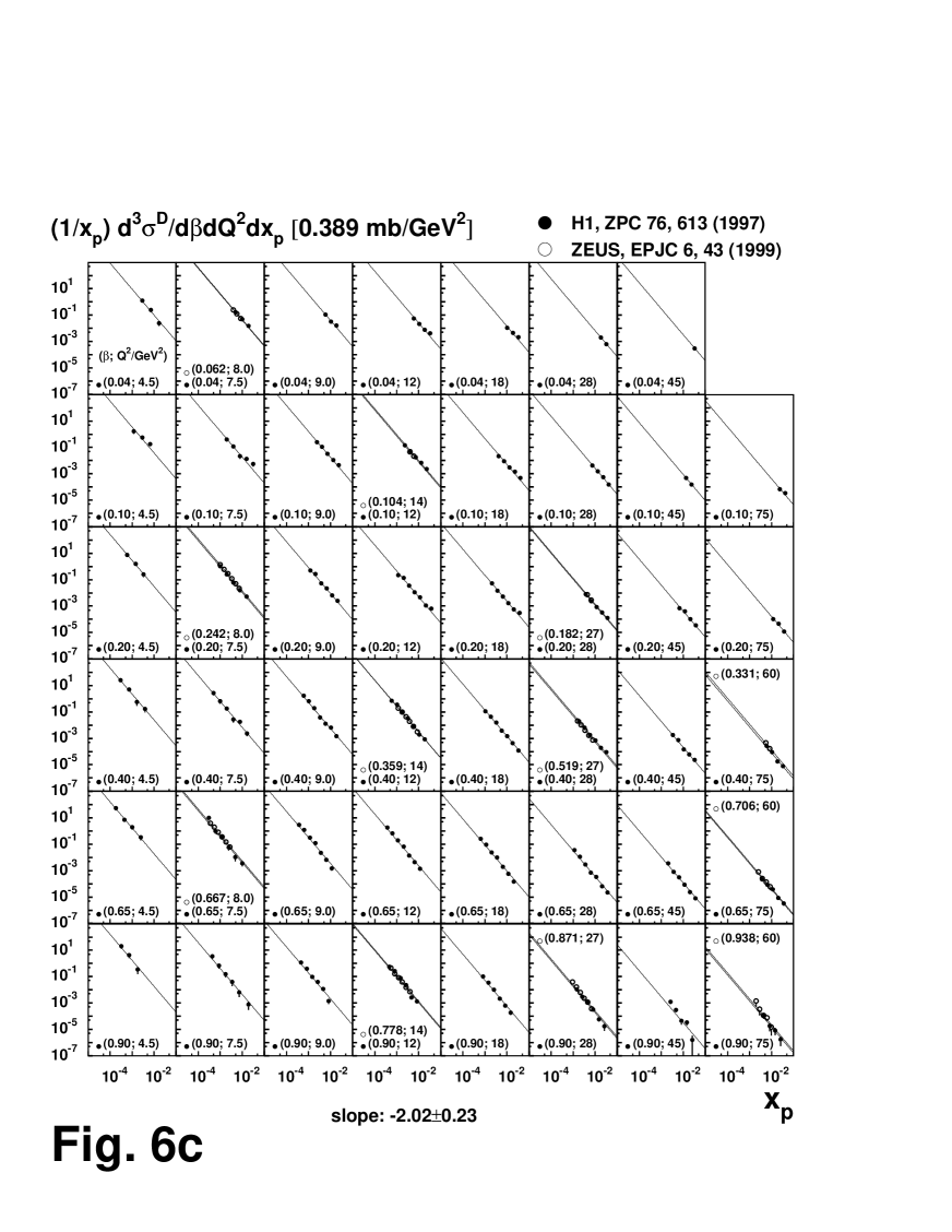
Figure 6: (a) $(1/x_{P})d^{3}\sigma^{D}/d\beta dQ^{2}dx_{P}$ is plotted as a function of $x_{P}$ in different bins of $\beta$ and $Q^{2}$. The data are taken from Ref.[References]. (The factor $0.389\,\mbox{mb}$ is due to $(1\,\mbox{GeV})^{-2}=0.389\,\mbox{mb}$.) (b) $(1/x_{P})d^{2}\sigma^{D}/dQ^{2}dx_{P}$ in units of $\mbox{GeV}^{-4}$ is plotted as a function of $x_{P}$ in different bins of $Q^{2}$. The data are taken from Ref.[References]. (c) same as (a) but with data taken from Ref.[References]. (The factor $0.389\,\mbox{mb}$ is due to $(1\,\mbox{GeV})^{-2}=0.389\,\mbox{mb}$.)

Together with Eqs.(3) and (8), we see that this cross-section is nothing else but the effective $\beta$-weighted $x_{P}$-distribution $D_{S}(x_{P}|Q^{2},\beta)$ of the $c_{0}^{\star}$’s. Note that the weighting factors shown on the right-hand-side of Eq.(15) are simply results of QED! Next, we use the data[3, 4] for $F_{2}^{D(3)}$ which are available at present, to do a log-log plot for the integrand of the expression in Eq.(15) as a function of $x_{P}$ for different values of $\beta$ and $Q^{2}$. This is shown in in Fig.6a and Fig.6c. Since the absolute values of this quantity depend very much, but the slope of the curves very little on $\beta$, we carry out the integration as follows: We first fit every set of the data separately. Having obtained the slopes and the intersection points, we use the obtained fits to perform the integration over $\beta$. The results are shown in the

$$\log{\left(\frac{1}{x_{P}}\,\frac{d^{2}\sigma^{D}}{dQ^{2}\,dx_{P}}\right)} \log{(x_{P})}$$   versus

plots of Fig.6b. These results show the $Q^{2}$-dependence of the slopes is practically negligible, and that the slope is approximately $-1.95$ for all values of $Q^{2}$.

Furthermore, in order to see whether the quantity introduced in Eq.(15) is indeed useful, and in order to perform a decisive test of the $Q^{2}$-independence of the slope in the power-law behavior of the above-mentioned size-distributions, we now compare the results in deep-inelastic scattering[3, 4] with those obtained in photoproduction[21], where LRG events have also been observed. This means, as in diffractive deep-inelastic scattering, we again associate the observed effects with colorless objects which are interpreted as a system of interacting soft gluons originating from the proton. In order to find out whether it is the same kind of gluon-clusters as in deep-inelastic scattering, and whether they “look” very much different when we probe them with real ($Q^{2}=0$) photons, we replot the existing $d\sigma/dM_{x}^{2}$ data[21] for photoproduction experiments performed at different total energies, and note the kinematical relationship between $M_{x}^{2}$, $W^{2}$ and $x_{P}$ (for $Q^{2}\ll M^{2}$ and $|t|\ll M_{x}^{2}$):

$$x_{P}\approx\frac{M_{x}^{2}}{W^{2}}$$ (16)

The result of the corresponding

$$\log{\left(\frac{1}{x_{P}}\,\frac{d\sigma}{dx_{P}}\right)} \log{(x_{P})}$$   versus

plot is shown in Fig.7. The slope obtained from a least-square fit to the existing data[21] is $-1.98\pm 0.07$.

The results obtained in diffractive deep-inelastic electron-proton scattering and that for diffractive photoproduction strongly suggest the following: The formation processes of $c_{0}^{\star}$’s in the proton is due to self-organized criticality, and thus the spatial distributions of such clusters — represented by the $x_{P}$-distribution — obey power-laws. The exponents of such power-laws are independent of $Q^{2}$. Since $1/Q^{2}$ can be interpreted as a measure for the transverse size of the incident virtual photon, the observed $Q^{2}$-independence of the exponents can be considered as further evidence for SOC — in the sense that the self-organized gluon-cluster formation processes take place independent of the photon which is “sent in” to detect the clusters.

Having these results, and the close relationship between real photons and hadrons in mind, we are immediately led to the following questions: What shall we see, when we replace the (virtual or real) photon by a hadron — a proton or an antiproton? (See in this connection Fig.8, for the notations and the kinematical relations for the description of such scattering processes.) Should we not see similar behaviors, if SOC in gluon-systems is indeed the reason for the occurrence of $c_{0}^{\star}$’s which can be probed experimentally in inelastic diffractive scattering processes? To answer these questions, we took a closer look at the available single diffractive proton-proton and proton-antiproton scattering data[5, 6]; and in order to make quantitative comparisons, we plot the quantities which correspond to those shown in Fig.6b and Fig.7. These plots are shown in Fig.9a and Fig.9b. In Fig.9a, we see the double differential cross-section $(1/x_{P})d^{2}\sigma/(dtdx_{P})$ at four different $t$-values. In Fig.9b, we see the integrated differential cross-section $(1/x_{P})d\sigma/dx_{P}$. Note that, here

$$x_{P}\approx M_{x}^{2}/s,$$ (17)

where $\sqrt{s}$ is the total c.m.s. energy of the colliding proton-proton or antiproton-proton system. Here, the integrations of the double differential cross-section over $t$ are in the ranges in which the corresponding experiments have been performed. (The extremely weak energy-dependence has been ignored in the integration.) The dashed lines in all the plots in Figs.9a and 9b stand for the slope $-1.97$ which is the average of the slope obtained from the plots shown in Figs.6b and 7. This means, the result shows exactly what we expect to see: The fingerprints of SOC can be clearly seen also in proton- and antiproton-induced inelastic diffractive scattering processes, showing that such characteristic features are indeed universal and robust!

We are thus led to the following conclusions. Color-singlet gluon-clusters ($c_{0}^{\star}$) can be formed in hadrons as a consequence of self-organized criticality (SOC) in systems of interacting soft gluons. In other words, “the colorless objects” which dominate the inelastic diffractive scattering processes are BTW-avalanches (BTW-clusters). Such $c_{0}^{\star}$’s are in general distributed partly inside and partly outside the confinement region of the “mother-hadron”. Since the interactions between the $c_{0}^{\star}$’s and other color-singlet objects (including the target proton) should be of Van der Waals type, it is expected that such an object can be readily driven out of the above-mentioned confinement region by the beam-particle in geometrically more peripheral collisions. This has been checked by examing inelastic single-diffractive scattering processes at high energies in which virtual photon, real photon, proton, and antiproton are used as beam particles. The result of this systematic check shows that the universal distributions of such $c_{0}^{\star}$’s can be directly extracted from the data. In particular, the fact that $x_{P}$ is the energy fraction carried by the struck $c_{0}^{\star}$’s, and the fact that the $x_{P}$-distributions are universal, it is tempting to regard such $x_{P}$-distributions as “the parton-distributions” for diffractive scattering processes. Having seen this, it is also tempting to ask: Can we make use of such “parton-distributions” to describe and/or to predict the measurable cross-sections in inelastic diffractive scattering processes? This and other related questions will be discussed in the following sections.

VIII Diffractive scattering in high-energy collisions and diffraction in optics

It might sound strange, but it is true that people working in this field of physics often do not agree with one another on the question: What is “Diffractive Scattering in High-Energy Collisions”? In this paper, we have, until now, simply adopted the currently [9] popular definition of “inelastic diffractive scattering processes”. That is, when we talked about “inelastic diffractive scattering” we were always referring to processes in which “colorless objects” are “exchanged”. In other words, until now, the following question has not been asked: Are the above-mentioned “inelastic diffractive scattering processes” indeed comparable with diffraction in Optics, in the sense that the beam particles should be considered as waves, and the target-proton together with the associated (in whatever manner) colorless objects can indeed be viewed as a “scattering screen”?

This question will be discussed in the present and the subsequent sections, together with the existing data [5, 22] for the double differential cross-section $d^{2}\sigma/dt\,d(M_{x}^{2}/s)$ for proton-proton and antiproton-proton collisions (where $t$ is the 4-momentum-transfer squared, $M_{x}$ is the missing-mass, and $\sqrt{s}$ is the total c.m.s. energy). The purpose of this investigation is to find out: “Can the observed $t$-dependence and the $(M_{x}^{2}/s)$-dependence of $d^{2}\sigma/dt\,d(M_{x}^{2}/s)$ in the given kinematic range ($0.2\mbox{\,GeV}^{2}$$\leq$$|t|$$\leq$ $3.25\mbox{\,GeV}^{2}$, $16\mbox{\,GeV}$$\leq$$\sqrt{s}$$\leq$ $630\mbox{\,GeV}$, and $M_{x}^{2}/s$$\leq$ $0.1$) be understood in terms of the well-known concept of diffraction in Optics? The answer to this question is of particular interest for several reasons:

(a) High-energy proton-proton and proton-antiproton scattering at small momentum transfer has played, and is still playing a very special role in understanding diffraction and/or diffractive dissociation in lepton-, photon- and hadron-induced reactions[2, 3, 4, 5, 6, 8, 9, 21, 22, 23, 24]. Many experiments have been performed at various incident energies for elastic and inelastic diffractive scattering processes. It is known that the double differential cross section $d^{2}\sigma/dt\,d(M_{x}^{2}/s)$ is a quantity which can yield much information on the reaction mechanism(s) and/or on the structure of the participating colliding objects. In the past, the $t$-, $M_{x}$- and $s$-dependence of the differential cross-sections for inelastic diffractive scattering processes has been presented in different forms, where a number of interesting features have been observed[5, 22, 23]. For example, it is seen that, the $t$-dependence of $d^{2}\sigma/dt\,dM_{x}^{2}$ at fixed $s$ depends very much on $M_{x}$; the $M_{x}^{2}$-dependence of $d^{2}\sigma/dt\,dM_{x}^{2}$ at fixed $t$ depends on $s$. But, when $d^{2}\sigma/dt\,d(M_{x}^{2}/s)$ is plotted as function of $M_{x}^{2}/s$ at given $t$ -values (in the range $0.2\,\mbox{GeV}^{2}\leq|t|\leq 3.25\,\mbox{GeV}^{2}$) they are approximately independent of $s$! What do these observed striking features tell us? The first precision measurement of this quantity was published more than twenty years ago[5]. Can this, as well as the more recent $d^{2}\sigma/dt\,d(M_{x}^{2}/s)$-data[22] be understood theoretically?

(b) The idea of using optical and/or geometrical analogies to describe high-energy hadron-nucleus and hadron-hadron collisions at small scattering angles has been discussed by many authors [24, 23] many years ago. It is shown in particular that this approach is very useful and successful in describing elastic scattering. However, it seems that, until now, no attempt has been made to describe the data[5, 22] by performing quantitative calculations for $d^{2}\sigma/dt\,d(M_{x}^{2}/s)$ by using optical geometrical analogies. It seems worthwhile to make such an attempt. This is because, it has been pointed out[12] very recently, that the above-mentioned analogy can be made to understand the observed $t$-dependence in $d\sigma/dt$.

(c) Inelastic diffractive $pp$- and $\bar{p}p$-scattering belongs to those soft processes which have also been extensivly discussed in the well-known Regge-pole approach[8, 9, 23]. The basic idea of this approach is that colorless objects in form of Regge trajectories (Pomerons, Reggeons etc.) are exchanged during the collision, and such trajectories are responsible for the dynamics of the scattering processes. In this approach, it is the $t$-dependence of the Regge trajectories, the $t$-dependence of the corresponding Regge residue functions, the properties of the coupling of the contributing trajectories (e.g. triple Pomeron or Pomeron-Reggeon-Pomeron coupling), and the number of contributing Regge trajectories which determine the experimentally observed $t$- and $M_{x}$-dependence of $d^{2}\sigma/dt\,d(M_{x}^{2}/s)$. A number of Regge-pole models[9, 8] have been proposed, and there exist good fits [9, 8] to the data. What remains to be understood in this approach is the dynamical origin of the Regge-trajectories on the one hand, and the physical meaning of the unknown functions (for example the $t$-dependence of any one of the Regge-residue functions) on the other. It has been pointed out [20, 12], that there may be an overlap between the “Partons in Pomeron and Reggeons” picture and the SOC-picture [12], and that one way to study the possible relationship between the two approaches is to take a closer look at the double differential cross-section $d^{2}\sigma/dt\,d(M_{x}^{2}/s)$.

IX Optical diffraction off dynamical complex systems

Let us begin our discussion on the above-mentioned questions by recalling that the concept of “diffraction” or “diffractive scattering” has its origin in Optics, and Optics is part of Electrodynamics, which is not only the classical limit, but also the basis of Quantum Electrodynamics (QED). Here, it is useful to recall in particular the following: Optical diffraction is associated with departure from geometrical optics caused by the finite wavelength of light. Frauenhofer diffraction can be observed by placing a scatterer (which can in general be a scattering screen with more than one aperture or a system of scattering objects) in the path of propagation of light (the wavelength of which is less than the linear dimension of the scatterer) where not only the light-source, but also the detecting device, are very far away from the scatterer. The parallel incident light-rays can be considered as plane waves (characterized by a set of constants $\vec{k},w\equiv|\vec{k}|$, and $u$ say, which denote the wave vector, the frequency and the amplitude of a component of the electromagnetic field respectively in the laboratory frame). After the scattering, the scattered field can be written in accordance with Huygens’ principle as

$$u_{P}=\frac{e^{i|\vec{k}^{\prime}|R}}{R}f(\vec{k},\vec{k}^{\prime}).$$ (18)

Here, $u_{P}$ stands for a component of the field originating from the scatterer, $\vec{k}^{\prime}$ is the wave vector of the scattered light in the direction of observation, $|\vec{k}^{\prime}|\equiv\omega^{\prime}$ is the corresponding frequency, $R$ is the distance between the scatterer and the observation point $P$, and $f(\vec{k},\vec{k}^{\prime}$) is the (unnormalized) scattering amplitude which describes the change of the wave vector in the scattering process. By choosing a coordinate system in which the $z$-axis coincides with the incident wave vector $\vec{k}$, the scattering amplitude can be expressed as follows[25, 24, 23]

$$f(\vec{q}) = \frac{1}{(2\pi)^{2}}\int\!\int\limits_{\mbox{}\Sigma}d^{2}\vec{b}\,\alpha(\vec{b})\,e^{-i\vec{q}\cdot\vec{b}}\mbox{\ .}$$ (19)

Here, $\vec{q}\equiv\vec{k}^{\prime}-\vec{k}$ determines the change in wave vector due to diffraction; $\vec{b}$ is the impact parameter which indicates the position of an infinitesimal surface element on the wave-front “immediately behind the scatterer” where the incident wave would reach in the limit of geometrical optics, and $\alpha(\vec{b})$ is the corresponding amplitude (associated with the boundary conditions which the scattered field should satisfy) in the two-dimensional impact-parameter-space (which is here the $xy$-plane), and the integration extends over the region $\Sigma$ in which $\alpha(\vec{b})$ is different from zero. In those cases in which the scatterer is symmetric with respect to the scattering axis (here the $z$-axis), Eq.(19) can be expressed, by using an integral representation for $J_{0}$, as

$$f(q) = \frac{1}{2\pi}\int\limits_{0}^{\infty}b\,db\,\alpha(b)J_{0}(qb)\mbox{\ .}$$ (20)

where $q$ and $b$ are the magnitudes of $\vec{q}$ and $\vec{b}$ respectively.

The following should be mentioned in connection with Eqs.(19) and (20): Many of the well-known phenomena related to Frauenhofer diffraction have been deduced[25] from these equations under the additional condition (which is directly related to the boundary conditions imposed on the scattered field) $|\vec{k}^{\prime}|=|\vec{k}|=\omega^{\prime}=\omega$, that is, $\vec{k}^{\prime}$ differs from $\vec{k}$ only in direction. In other words, the outgoing light wave has exactly the same frequency, and exactly the same magnitude of wave-vector as those for the incoming wave. (This means, quantum mechanically speaking, the outgoing photons are also on-shell photons, the energies of which are the same as the incoming ones.) In such cases, it is possible to envisage that $\vec{q}$ is approximately perpendicular to $\vec{k}$ and to $\vec{k}^{\prime}$, that is, $\vec{q}$ is approximately perpendicular to the chosen $z$-axis, and thus in the above-mentioned $xy$-plane (that is $\vec{q}\approx\vec{q}_{\perp}$). While the scattering angle distribution in such processes (which are considered as the characteristic features of elastic diffractive scattering) plays a significant role in understanding the observed diffraction phenomena, it is of considerable importance to note the following:

(A) Eqs.(19) and (20) can be used to describe diffractive scattering with, or without, this additional condition, provided that the difference of $\vec{k}^{\prime}$ and $\vec{k}$ in the longitudinal direction (i.e. in the direction of $\vec{k}$) is small compared to $q_{\perp}\equiv|\vec{q}_{\perp}|$ so that $\vec{q}_{\perp}$ can be approximated by $\vec{q}$. In fact, Eqs.(19) and (20) are strictly valid when $\vec{q}$ is a vector in the above-mentioned $xy$-plane, that is when we write $\vec{q}_{\perp}$ instead of $\vec{q}$. Now, since Eqs.(19) and (20) in such a form (that is when the replacement $\vec{q}\rightarrow\vec{q}_{\perp}$ is made) are valid without the condition $\vec{q}$ should approximately be equal to $\vec{q}_{\perp}$ and in particular without the additional condition $|\vec{k}^{\prime}|=|\vec{k}|=\omega^{\prime}=\omega$, it is clear that they are also valid for inelastic scattering processes. In other words, Eqs.(19) and (20) can also be used to describe inelastic diffractive scattering (that is, processes in which $\omega^{\prime}\neq\omega$, $|\vec{k}^{\prime}|\neq|\vec{k}|$) provided that the following replacements are made. In Eq.(19), $\vec{q}\rightarrow\vec{q}_{\perp}$, $f(\vec{q})\rightarrow f_{\mbox{\tiny inel.}}(\vec{q}_{\perp})$, $\alpha(\vec{b})\rightarrow\alpha_{\mbox{\tiny inel.}}(\vec{b})$; and in Eq.(20) $q\rightarrow q_{\perp}$, $f(q)\rightarrow f_{\mbox{\tiny inel.}}(q_{\perp})$, $\alpha(b)\rightarrow\alpha_{\mbox{\tiny inel.}}(b)$. Hereafter, we shall call Eqs.(19) and (20) with these replacements Eq.(19^′) and Eq.(20^′) respectively. We note, in order to specify the dependence of $f_{\mbox{\tiny inel.}}$ on $\omega^{\prime}$ and $k_{\|}^{\prime}$ (that is on $\omega^{\prime}-\omega$ and $k_{\|}^{\prime}-k_{\|}$), further information on energy-momentum transfer in such scattering processes is needed. This point will be discussed in more detail in Section X.

(B) In scattering processes at large momentum-transfer where the magnitude of $\vec{q}_{\perp}$ is large ($|\vec{q}_{\perp}|^{2}\gg 0.05\,\mbox{GeV}^{2}$, say), it is less probable to find diffractive scattering events in which the additional condition $|\vec{k}^{\prime}|=|\vec{k}|$ and $\omega^{\prime}=\omega$ can be satisfied. This means, it is expected that most of the diffraction-phenomena observed in such processes are associated with inelastic diffractive scattering.

(C) Change in angle but no change in magnitude of wave-vectors or frequencies is likely to occur in processes in which neither absorption nor emission of light takes place. Hence, it is not difficult to imagine, that the above-mentioned condition can be readily satisfied in cases where the scattering systems are time-independent macroscopic apertures or objects. But, in this connection, we are also forced to the question: “How large is the chance for a incident wave not to change the magnitude of its wave-vector in processes in which the scatterers are open, dynamical, complex systems, where energy- and momentum-exchange take place at anytime and everywhere?!”

The picture for inelastic diffractive scattering has two basic ingredients:

First, having the well-known phenomena associated with Frauenhofer’s diffraction and the properties of de Broglie’s matter waves in mind, the beam particles ($\gamma^{\star}$, $\gamma$, $\overline{p}$ or $p$ shown in Fig.8) in these scattering processes are considered as high-frequency waves passing through a medium. Since, in general, energy- and momentum-transfer take place during the passage through the medium, the wave-vector of the outgoing wave differs, in general, from the incoming one, not only in direction, but also in magnitude. For the same reason, the frequency and the longitudinal component of the wave-vector of the outgoing wave (that is the energy, and/or the invariant mass, as well as the longitudinal momentum of the outgoing particles) can be different from their incoming counterparts.

Second, according to the results obtained in Sections I-VII of this paper, the medium is a system of color-singlet gluon-clusters ($c_{0}^{\star}$’s) which are in general partly inside and partly outside the proton — in form of a “cluster cloud”. Since the average binding energy between such color-singlet aggregates are of Van der Waals type[26], and thus it is negligibly small compared with the corresponding binding energy between colored objects, we expect to see that, even at relatively small values of momentum-transfer ($|t|$$<$$1\,\mbox{GeV}^{2}$,say), the struck $c_{0}^{\star}$ can unify with (be absorbed by) the beam-particle, and “be carried away” by the latter, similar to the process of “knocking out nucleons” from nuclear targets in high-energy hadron-nucleus collisions. It should, however, be emphasized that, in contrast to the nucleons in nucleus, the $c_{0}^{\star}$’s which can exist inside or outside the confinement-region of the proton are not hadron-like (See Sections III-VI for more details). They are BTW-avalanches which have neither a typical size, nor a typical lifetime, nor a given static structure. Their size- and lifetime-distributions obey simple power-laws as consequence of SOC. This means, in the diffraction processes discussed here, the size of the scatterer(s), and thus the size of the carried-away $c_{0}^{\star}$ is in general different in every scattering event. It should also be emphasized that these characteristic features of the scatterer are consequences of the basic properties of the gluons.

X Can such scattering systems be modeled quantitatively?

To model the proposed picture quantitatively, it is convenient to consider the scattering system in the rest frame of the proton target. Here, we choose a right-handed Cartesian coordinate with its origin $O$ at the center of the target-proton, and the $z$-axis in the direction of the incident beam. The $xy$-plane in this coordinate system coincides with the two-dimensional impact-parameter space mentioned in connection with Eqs.(19^′) and (20^′) [which are respectively Eq.(19) and Eq.(20) after the replacements mentioned in (A) below Eq.(20)], while the $yz$-plane is the scattering plane. We note, since we are dealing with inelastic scattering (where the momentum transfer, including its component in the longitudinal direction, can be large; in accordance with the uncertainty principle) it is possible to envisage that (the c.m.s. of) the incident particle in the beam meets $c_{0}^{\star}$’s at one point $B\equiv(0,b,z)$. where the projection of $\overline{OB}$ along the $y$-axis characterizes the corresponding impact parameter $\vec{b}$. We recall that such $c_{0}^{\star}$’s are avalanches initiated by local perturbations (caused by local gluon-interactions associated with absorption or emission of one or more gluons; see Sections I - VII for details) of SOC states in systems of interacting soft gluons. Since gluons carry color, the interactions which lead to the formation of color-singlet gluon-clusters ($c_{0}^{\star}$) must take place inside the confinement region of the proton. This means, while a considerable part of such $c_{0}^{\star}$’s in the cloud can be outside the proton, the location $A$, where such an avalanche is initiated, must be inside the proton. That is, in terms of $\overline{OA}\equiv r$, $\overline{AB}\equiv R_{A}(b)$, and proton’s radius $r_{p}$, we have $r\leq r_{p}$ and $[R_{A}(b)]^{2}=b^{2}+z^{2}+r^{2}-2(b^{2}+z^{2})^{1/2}r\cos\angle BOA$. For a given impact parameter $b$, it is useful to know the distance $R_{A}(b)$ between $B$ and $A$, as well as “the average squared distance” $\langle R_{A}^{2}(b)\rangle=b^{2}+z^{2}+a^{2}$, $a^{2}\equiv 3/5\,r_{p}^{2}$, which is obtained by averaging over all allowed locations of $A$ in the confinement region. That is, we can model the effect of confinement in cluster-formation by picturing that all the avalanches, in particular those which contribute to scattering events characterized by a given $b$ and a given $z$ are initiated from an “effective initial point” $\langle A_{B}\rangle$, because only the mean distance between $A$ and $B$ plays a role. (We note, since we are dealing with a complex system with many degrees of freedom, in which $B$ as well as $A$ are randomly chosen points in space, we can compare the mean distance between $B$ and $A$ with the mean free path in a gas mixture of two kinds of gas molecules — “Species $B$” and “Species $A$” say, where those of the latter kind are confined inside a subspace called “region $p$”. For a given mean distance, and a given point $B$, there is in general a set of $A$’s inside the “region $p$”, such that their distance to $B$ is equal to the given mean value. Hence it is useful to introduce a representative point $\langle A_{B}\rangle$, such that the distance between $\langle A_{B}\rangle$ and $B$ is equal to the given mean distance.) Furthermore, since an avalanche is a dynamical object, it may propagate within its lifetime in any one of the $4\pi$ directions away from $\langle A_{B}\rangle$. (Note: avalanches of the same size may have different lifetimes, different structures, as well as different shapes. The location of an avalanche in space-time is referred to its center-of-mass.) Having seen how SOC and confinement can be implemented in describing the properties and the dynamics of the $c_{0}^{\star}$’s, which are nothing else but BTW-avalanches in systems of interacting soft gluons, let us now go one step further, and discuss how these results can be used to obtain the amplitudes in impact-parameter-space that leads, via Eq.(20), to the scattering amplitudes.

In contrast to the usual cases, where the scatterer in the optical geometrical picture of a diffractive scattering process is an aperture, or an object, with a given static structure, the scatterer in the proposed picture is an open, dynamical, complex system of $c_{0}^{\star}$’s. This implies in particular: The object(s), which the beam particle hits, has (have) neither a typical size, nor a typical lifetime, nor a given static structure.

With these in mind, let us now come back to our discussion on the double differential cross section $d^{2}\sigma/dt\,d(M_{x}^{2}/s)$. Here, we need to determine the corresponding amplitude $\alpha_{\mbox{\tiny inel.}}(b)$ in Eq.(20^′) [see the discussion in (A) below Eq.(20)]. What we wish to do now, is to focus our attention on those scattered matter-waves whose de Broglie wavelengths are determined by the energy-momentum of the scattered object, whose invariant mass is $M_{x}$. For this purpose, we characterize the corresponding $\alpha_{\mbox{\tiny inel.}}(b)$ by considering it as a function of $M_{x}$, or $M_{x}^{2}/s$, or $x_{P}$. We recall in this connection that, for inelastic diffractive scattering processes in hadron-hadron collisions, the quantity $M_{x}^{2}/s$ is approximately equal to $x_{P}$, which is the momentum fraction carried by the struck $c_{0}^{\star}$’s with respect to the incident beam (see Fig.8 for more details; note however that $q_{c}$, $k$ and $p_{x}$ in Fig.8 correspond respectively to $q$, $k$ and $k^{\prime}$ in the discussions here.). Hence, we shall write hereafter $\alpha(b\,|M_{x}^{2}/s)$ or $\alpha(b\,|x_{P})$ instead of the general expression $\alpha_{\mbox{\tiny inel.}}(b)$. This, together with Eq.(20^′), leads to the corresponding scattering amplitude $f(q_{\bot}|x_{P})$, and thus to the corresponding double differential cross-section $d^{2}\sigma/dt\,dx_{P}$, in terms of the variables $|t|\approx|\vec{q}_{\bot}|^{2}$ and $x_{P}\approx M_{x}^{2}/s$ in the kinematical region: $|t|\ll M_{x}^{2}\ll s$.

XI The role played by the space-time properties of the gluon-clusters

For the determination of $\alpha(b\,|x_{P})$, it is of considerable importance to recall the following space-time properties of the $c_{0}^{\star}$’s which are BTW-avalanches due to SOC:

(i) SOC dictates, that there are BTW-avalanches of all sizes (which we denote by different $S$ values), and that the probability amplitude of finding an avalanche of size $S$ can be obtained from the size-distribution $D_{S}(S)=S^{-\mu}$ where the experimental results presented in Sections I - VII show: $\mu\approx 2$. This means, $D_{S}(S)$ contributes a factor $S^{-1}$, thus a factor $x_{P}^{-1}$ to the scattering amplitude $\alpha(b\,|x_{P})$. Here, as well as in (ii), we take into account (see Sections IV and V for details) that the size $S$ of a $c_{0}^{\star}$ is directly proportional to the total amount of the energy the $c_{0}^{\star}$ carries; the amount of energy is $x_{P}P^{0}$, where $P^{0}$ is the total energy of the proton, and $x_{P}$ is the energy fraction carried by the $c_{0}^{\star}$.

(ii) QCD implies[26] that the interactions between two arbitrarily chosen colored constituents of $c_{0}^{\star}$ is stronger than those between two $c_{0}^{\star}$’s, because the latter should be interactions of Van der Waals type. This means, the struck $c_{0}^{\star}$ can unify with the beam-particle (maybe by absorbing each other), and viewed from any Lorentz frame in which the beam-particle has a larger momentum than the $c_{0}^{\star}$, the latter is “carried away” by the beam particle. Geometrically, the chance for the beam-particle to hit an $c_{0}^{\star}$ of size $S$ ( on the plane perpendicular to the incident axis) is proportional to the area that can be struck by the (c.m.s.) of the beam particle. The area is the $2/3$-power of the volume $S$, $S^{2/3}$, and thus it is proportional to $x_{P}^{2/3}$.

(iii) Based on the above-mentioned picture in which the $c_{0}^{\star}$’s propagate isotropically from $\langle A_{B}\rangle$, the relative number-densities at different $b$-values can be readily evaluated. Since for a given $b$, the distance in space between $\langle A_{B}\rangle$ and $B\equiv(0,b,z)$ is simply $(b^{2}+z^{2}+a^{2})^{1/2}$, the number of $c_{0}^{\star}$’s which pass a unit area on the shell of radius $(b^{2}+z^{2}+a^{2})^{1/2}$ centered at $\langle A_{B}\rangle$ is proportional to $(b^{2}+z^{2}+a^{2})^{-1}$, provided that (because of causality) the lifetimes ($T$’s) of these $c_{0}^{\star}$’s are not shorter than $\tau_{\mbox{\tiny min}}(b)$. The latter is the time interval for a $c_{0}^{\star}$ to travel from $\langle A_{B}\rangle$ to $B$. This means, because of the space-time properties of such $c_{0}^{\star}$’s, it is of considerable importance to note: First, only $c_{0}^{\star}$’s having lifetimes $T\geq\tau_{\mbox{\tiny min}}(b)$ can contribute to such a collision event. Second, during the propagation from $\langle A_{B}\rangle$ to $B$, the motion of such a $c_{0}^{\star}$ has to be considered as Brownian. In fact, the continual, and more or less random, impacts received from the neighboring objects on its path leads us to the well known [27] result that the time elapsed is proportional to the mean-square displacement. That is: $\tau_{\mbox{\tiny min}}(b)\propto b^{2}+z^{2}+a^{2}$. Furthermore, we recall that $c_{0}^{\star}$’s are due to SOC, and thus the chance for a $c_{0}^{\star}$ of lifetime $T$ to exist is $D_{T}(T)\propto T^{-\nu}$ where the experimental value (see Sections I - VII) for $\nu$ is $\nu\approx 2$. Hence, by integrating $T^{-2}$ over $T$ from $\tau_{\mbox{\tiny min}}(b)$ to infinity, we obtain the fraction associated with all those whose lifetimes satisfy $T\geq\tau_{\mbox{\tiny min}}(b)$: This fraction is $\tau_{\mbox{\tiny min}}(b)^{-1}$, and thus a constant times $(b^{2}+z^{2}+a^{2})^{-1}$.

The amplitude $\alpha(b\,|x_{P})$ can now be obtained from the probability amplitude for $c_{0}^{\star}$-creation mentioned in (i), by taking the weighting factors mentioned in (ii) and (iii) into account, and by integrating[28] over $z$ . The result is:

$$\alpha(b\,|x_{P})=\mbox{const.}x_{P}^{-1/3}(b^{2}+a^{2})^{-3/2}\mbox{\,.}$$ (21)

By inserting this probability amplitude in impact-parameter-space, for the beam particle to encounter a $c_{0}^{\star}$, which carries a fraction $x_{P}$ of the proton’s total energy, in Eq.(20^′) [which is Eq.(20) with the following replacements: $q\rightarrow q_{\perp}$, $f(q)\rightarrow f_{\mbox{\tiny inel.}}(q|x_{P})$ and $\alpha(b)\rightarrow\alpha_{\mbox{\tiny inel.}}(b|x_{P})$] we obtain the corresponding probability amplitude $f(q|x_{P})$ in momentum-space:

$$f(q_{\bot}|x_{P})=\mbox{const.}\int_{0}^{\infty}b\,db\,x_{P}^{-1/3}(b^{2}+a^{2})^{-3/2}J_{0}(q_{\bot}b),$$ (22)

where $q_{\bot}=|\vec{q}_{\bot}|\approx\sqrt{|t|}$ (in the small $x_{P}$-region, $x_{P}<0.1$, say) is the corresponding momentum-transfer. The integration can be carried out analytically[29], and the result is

$$f(q_{\bot}|x_{P})={\rm const.}x_{P}^{-1/3}\exp(-aq_{\bot})\mbox{\,.}$$ (23)

Hence, the corresponding double differential cross-section $d^{2}\sigma/dtdx_{P}$ can approximately be written as

$$\frac{1}{\pi}{d^{2}\sigma\over dt\,dx_{P}}=Nx_{P}^{-2/3}\exp(-2a\sqrt{|t|}),$$ (24)

where $N$ is an unknown normalization constant. Because of the kinematical relationship $x_{P}\approx M_{x}^{2}/s$ for single diffractive scattering in proton-proton and proton-antiproton collisions (see Fig.8 for more details), this can be, and should be, compared with the measured double differential cross-sections $d^{2}\sigma/dt\,d(M_{x}^{2}/s)$ at different $t$- and $s$-values and for different missing masses $M_{x}$ in the region $M_{x}^{2}/s\ll 1$ where $q_{\perp}$ is approximately $\sqrt{|t|}$. The comparison is shown in Fig.10. Here, we made use of the fact that $a^{2}\equiv 3/5\,r_{p}^{2}$, where $r_{p}$ is the proton radius, and calculated $a$ by setting $r_{p}^{2}$ to be the well-known [30] mean square proton charge radius, the value of which is $r_{p}^{2}=(0.81\,\mbox{fm})^{2}$. The result we obtained is: $a=3.2\,\mbox{GeV}^{-1}$. The unknown normalization constant is determined by inserting this calculated value for $a$ in Eq.(24), and by comparing the right-hand-side of this equation with the $d^{2}\sigma/dt\,d(M_{x}^{2}/s)$ data taken at $|t|=0.2\,\mbox{GeV}^{2}$. The value is $N=31.1\,\mbox{mb GeV}^{-2}$. All the curves shown in Fig.10 are obtained by inserting these values for $a$ and $N$ in Eq.(24).

While the quality of the obtained result, namely the expression given on the right-hand-side of Eq.(24) together with the above-mentioned values for $a$ and $N$, can be readily judged by comparing it with the data, or by counting the unknown parameters, or both, it seems worthwhile to recall the following: The two basic ingredients of the proposed picture which have been used to derive this simple analytical expression are: first, the well-known optical analogy, and second, the properties of the dynamical scattering system. The latter is what we have learned through the data-analysis presented in Sections I - VII.

Based on the theoretical arguments and experimental indications for the observation (see Ref.[References] and Section I - VII of this paper for details) that the characteristic features of inelastic diffractive scattering processes are approximately independent of the incident energy and independent of the quantum-numbers of the beam-particles, the following results are expected: The explicit formula for the double differential cross-section as shown in Eq.(24) should also be valid for the reactions $\gamma p\rightarrow Xp$ and $\gamma^{\star}p\rightarrow Xp$. While the normalization constant $N$ (which should in particular depend on the geometry of the beam particle) is expected to be different for different reactions, everything else – especially the “slope” as well as the power of $x_{P}$ should be exactly the same as in $pp$- and $p\bar{p}$-collisions. In this sense, Eq.(24) with $a^{2}=3/5r_{P}^{2}$ ($r_{P}$ is the proton radius) is our prediction for $\gamma p\rightarrow Xp$ and $\gamma^{\star}p\rightarrow Xp$ which can be measured at HERA.

Furthermore, in order to obtain the integrated differential cross-section $d\sigma/dt$, which has also been measured for different reactions at different incident energies, we only need to sum/integrate over $x_{P}$ in the given kinematic range ($x_{P}<0.1$, say). The result is

$${d\sigma\over dt}(t)=C\exp(-2a\sqrt{|t|}),$$ (25)

where $C$ is an unknown normalization constant. While this observation has already been briefly discussed in the previous Letter [12], we now show the result of a further test of its universality: In Fig.11, we plot

$$-{1\over 2\sqrt{|t|}}\log[\frac{1}{C}\,{d\sigma\over dt}(t)]\mbox{ vs. }t$$ (26)

for different reactions at different incident energies in the range $0.2$$\mbox{\,GeV}^{2}$$\leq$$|t|$$\leq 4\mbox{\,GeV}^{2}$. Here we see in particular that, measurements of $d\sigma/dt$ for $\gamma^{\star}p$ and $\gamma p$ reactions at larger $|t|$-values would be very useful.

XII Concluding remarks

Based on the characteristic properties of the gluons — in particular the local gluon-gluon coupling prescribed by the QCD-Lagrangian, the confinement, and the non-conservation of gluon-numbers, we suggest that a system of interacting soft gluons should be considered as an open dynamical complex system which is in general far away from equilibrium. Taken together with the observations made by Bak, Tang and Wiesenfeld (BTW) [13, 14], we are led to the conclusion, that self-organized criticality (SOC) and thus BTW-avalanches exist in such systems, and that such avalanches manifest themselves in form of color-singlet gluon-clusters ($c_{0}^{\star}$) in inelastic diffractive scattering processes.

In order to test this proposal, we performed a systematic data-analysis, the result of which is presented in Sections I - VII: It is shown that the size-distributions, and the lifetime-distributions, of such $c_{0}^{\star}$’s indeed exhibit power-law behaviors which are known as the fingerprints of SOC [13, 14]. Furthermore, it is found that such exponents are approximately the same for different reactions and/or at different incident energies — indicating the expected universality and robustness of SOC. Hence, the following picture emerges: For the beam particle (which may be a virtual photon, or a real photon, or a proton, or an antiproton; see Fig.8 for more details) in an inelastic diffractive scattering process off proton (one may wish to view this from a “fast moving frame” such as the c.m.s. frame), the target proton appears as a cloud of $c_{0}^{\star}$’s which exist inside and outside the confinement region of the proton. The size-distribution $D_{S}(S)$ and the lifetime-distribution $D_{T}(T)$ can be expressed as $S^{-\mu}$ and $T^{-\nu}$ respectively, where the empirical values for $\mu$ and $\nu$ are $\mu$$\approx$$\nu$$\approx$$2$, independent of the incident energy, and independent of the quantum numbers of the beam particles.

What do we learn from this? Is this knowledge helpful in understanding hadronic structure and/or hadronic reactions in Particle Physics? In particular, can this knowledge be used to do quantitative calculations — especially those, the results of which could not be achieved otherwise?

In order to demonstrate how the obtained knowledge can be used to relate hadron-structure and hadronic reactions in general, and to perform quantitative calculations in particular, we discuss the following question — a question which has been with the high-energy physics community for many years:

“Can the measured double differential cross section $d^{2}\sigma/dt\,d(M_{x}^{2}/s)$ for inelastic diffractive scattering in proton-proton and in antiproton-proton collisions, in the kinematical region given by $0.2\mbox{\,GeV}^{2}$$\leq$$|t|$$\leq$ $3.25\mbox{\,GeV}^{2}$, $16\mbox{\,GeV}$$\leq$$\sqrt{s}$$\leq$ $630\mbox{\,GeV}$, and $M_{x}^{2}/s$ $\leq$$0.1$, be understood in terms of optical geometrical concepts?”

The answer to this question is “Yes!”, and the details are presented in Sections IX - XI where the following is explicitly shown: The characteristic features of the existing $d^{2}\sigma/dt\,d(M_{x}^{2}/s)$-data are very much the same as those in optical diffraction, provided that the high-energy beams are considered as high-frequency waves, and the scatterer is a system of color-singlet gluon-clusters ($c_{0}^{\star}$) described in Sections I - VII of this paper. Further measurements of double differential cross sections, especially in $\gamma^{\star}p$- and $\gamma p$-reactions, will be helpful in testing the ideas presented here.

Figure 2: $F_{2}^{D(3)}(\beta,Q^{2};x_{P})/\beta$ is plotted as a function of $\beta$ for given $x_{P}$-intervals and for fixed $Q^{2}$-values. The data are taken from Ref.[References]. The lines are only to guide the eye.

Figure 3: (a) $F_{2}^{D(3)}(\beta,Q^{2};x_{P})/x_{P}$ is plotted as a function of $x_{P}$ for different values of $\beta$ and $Q^{2}$. The data are taken from Ref.[References]. (b) same as (a) but with data taken from Ref.[References]. Note that in these log-log plots, almost all existing data points lie on straight-lines with approximately the same slope irrespective of the values of $Q^{2}$ and/or $\beta$.

Figure 4: $F_{2}^{D(3)}(\beta,Q^{2};x_{P})/\beta$ is plotted as a function of $x_{B}$ in the indicated $\beta$- and $Q^{2}$-ranges. The data are taken from Ref.[References].

Figure 5: (a) $F_{2}^{D(3)}(\beta,Q^{2};x_{B}/\beta)/(\beta x_{B})$ is plotted as a function of $x_{B}$ for fixed $\beta$- and $Q^{2}$-values. The data are taken from Ref.[References]. (b) same as (a) but with data taken from Ref.[References]. Note that in these log-log plots, almost all existing data points lie on straight-lines with approximately the same slope irrespective of the values of $Q^{2}$ and/or $\beta$.

Figure 7: $(1/x_{P})d\sigma/dx_{P}$ for photoproduction $\gamma+p\rightarrow X+p$ is plotted as a function of $x_{P}$. The data are taken from Ref.[References]. Note that the data in the second paper are given in terms of relative cross sections. Note also that the slopes of the straight-lines are the same. The two dashed lines indicate the lower and the upper limits of the results obtained by multiplying the lower solid line by $\sigma_{\mbox{tot}}=154\pm 16\mbox{(stat.)}\pm 32\mbox{(syst.)}\mu b$. This value is taken from the third paper in Ref.[References].

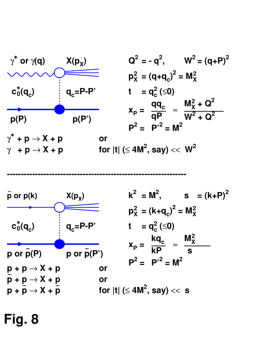
Figure 8: Diagrams for different single diffractive reactions, together with the definitions of the relevant kinematic variables.

Figure 9: a) $(1/x_{P})d^{2}\sigma/dx_{P}dt$ for single diffractive $p+p\rightarrow p+X$ and $p+\bar{p}\rightarrow p+X$ reactions is plotted as a function of $x_{P}$ at different values of $t$ and $\sqrt{s}$. The data are taken from Ref.[References,References]. b) The integrated (with respect to two different $|t|$-ranges) differential cross section $(1/x_{P})d\sigma/dx_{P}$ for single diffractive $p+p\rightarrow p+X$ and $p+\bar{p}\rightarrow p+X$ reactions is plotted as a function of $x_{P}$.

Figure 10: The double differential cross section $(1/\pi)\,d^{2}\sigma/dt\,d(M_{x}^{2}/s)$ for single diffractive $pp$ and $\bar{p}p$ reactions is shown as function of $x_{P}$ at fixed values of $t$ where $0.15$$\mbox{\,GeV}^{2}$$\leq$$|t|$$\leq$$3.25$$\mbox{\,GeV}^{2}$. The data are taken from Refs. [References,References]. The solid curve is the result obtained from Eq.(24). The dashed curve stands for the result obtained from the same formula by using the $t$-value given in the bracket.

Figure 11: The quantity $(-1/(2\sqrt{|t|}))\log{[\frac{1}{C}\,d\sigma/dt]}$ is plotted versus $\sqrt{|t|}$ for different single diffractive reactions in the range $0.2$$\mbox{\,GeV}^{2}$$\leq$$|t|$$\leq$$4$$\mbox{\,GeV}^{2}$. The data are taken from Refs. [References,References,References]. Here, $C$, the normalization constant is first determined by performing a two-parameter fit of the corresponding $d\sigma/dt$-data to Eq.(25).

References

- [1] See for example: S. Aid, et al., H1 Coll., Phys. Lett. B354, 494 (1995); M. Derrick, et al., ZEUS Coll., Phys. Lett. B345, 576 (1995); and the papers cited therein.
- [2] M. Derrick, et al., ZEUS Coll., Phys. Lett. B315, 481 (1993); T. Ahmed, et al., H1 Coll., Nucl. Phys. B429, 477 (1994).
- [3] T. Ahmed, et al., H1 Coll., Phys. Lett. B348, 681 (1995); M. Derrick, et al., ZEUS Coll., Z. Phys. C68, 569 (1995); ibid, C70, 391 (1996); J. Phillips, in Proceeding of the 28th Int. Conf. on High-Energy Physics, Warsaw, 1996, edited by Z. Ajduk and A. K. Wroblewski (World Scientific, 1997) Vol.1, p. 623; and the papers cited therein;
- [4] C. Adloff et al., H1 Coll., Z.Phys. C76, 613 (1997); J. Breitweg et al., ZEUS Coll., Europ.Phys.J. C6, 43 (1999).
- [5] M.G. Albrow, et al., Nucl. Phys. B108, 1 (1976); R. D. Schamberger, et al., Phys. Rev. D17, 1268 (1978).
- [6] R. L. Cool, et al., Phys. Rev. Lett. 47, 701 (1981); F. Abe, et al., CDF Coll., Phys. Rev. D50, 5535 (1994); K. Goulianos, in Proceedings of DIS97, Chicago, 1997, edited J. Repond and D. Krakauer, (AIP), p.527.
- [7] S. Abachi, et al., D0 Coll., Phys. Rev. Lett. 72, 2332 (1994); Phys. Rev. Lett. 76, 734 (1996); F. Abe, et al., CDF Coll., Phys. Rev. Lett. 74, 855 (1995).
- [8] See in particular: F.E.Low, Phys. Rev. D12, 163 (1975); S. Nussinov, Phys. Rev. Lett.34, 1286 (1975); G. Ingelman, P.Schlein, Phys. Lett. B152, 256 (1985); A. Donnachie, P.V. Landshoff, Phys. Lett. B191, 309 (1987); Y.A.Simonov, Phys. Lett. B249, 514 (1990); G. Ingelman, K. Janson-Prytz, Phys. Lett. B281, 325 (1992); G.Ingelman, K.Prytz, Z. Phys. C58, 285 (1993); and the papers cited therein.
- [9] See for example: J. Bartels, in Proceedings of the 17th Int. Symp. on Lepton-Photon Interactions, Beijing, 1995, edited by Zheng Zhi-peng and Chen He-sheng, (World Scientific, 1996), Vol. 2, p. 554; H. Abramowicz, J. Bartels, L. Frankfurt and H. Jung, in Proceedings of the Workshop on Future Physics at HERA, edited by G. Ingelman, A. De Roeck, R. Klanner, (publ. by DESY), Vol. 2, p. 535; E. Gallo, in Proceedings of the 18th Int. Symp. on Lepton - Photon Interactions, Hamburg, 1997, edited by A. DeRoeck and A. Wagner, (World Scientific, Singapore 1998); and the references given therein; M. Erdmann, in Proceedings of the 29th International Conference on High Energy Physics, Vancouver, 1998, (in press).
- [10] M. Derrick, et al., ZEUS Coll., Phys. Lett. B332, 228 (1994); Phys. Lett. B346, 399 (1995); S. Aid, et al., H1 Coll., Nucl. Phys. B445, 3 (1995).
- [11] C. Boros, Z. Liang and T. Meng, Phys. Rev. D54, 6658 (1996).
- [12] T.Meng, R. Rittel and Y. Zhang, Phys. Rev. Lett. 82, 2044 (1999).
- [13] P. Bak, C. Tang and K. Wiesenfeld, Phys. Rev. Lett. 59, 381 (1987); Phys. Rev. A38, 364 (1988).
- [14] See for example the recent review article by P. Bak and M. Creutz, in Fractals in Science, edited by A. Bunde and S. Havlin (Springer, New York, Berlin, Heidelberg 1994); P. Bak, How nature works, (Springer, New York 1996); H. J. Jensen, Self-Organized Criticality, (Cambridge University Press, Cambridge 1998); and the papers cited therein (as mentioned by Bak in the Preface of his book, since 1987, more than 2000 papers have been written on self-organized criticality; we apologize to all the authors whom we did not quote here).
- [15] P. Bak and C. Tang, J. Geophys. Res. B94, 15635 (1989); K. Ito and M. Mastsuzaki, J. Geophys. Res. B95, 6853 (1989); Z. Olami, H. J. Feder, K. Christensen, Phys. Rev. Lett.68, 1244 (1992).
- [16] P. Bak, K. Chen and M. Creutz, Nature 342, 780 (1989).
- [17] P. Bak and K. Sneppen, Phys. Rev. Lett. 71, 4083 (1993).
- [18] H. Flyvbjerg, K. Sneppen and P. Bak, Phys. Rev. Lett. 71, 4087 (1993); M. Paczuski, S. Maslov and P. Bak, Europhys. Lett. 27, 97 (1994); B. Jovanovic, S. V. Buldyrev, S. Havlin and H. E. Stanley, Phys. Rev. E50, 2403 (1994); P. Grassberger, Phys. Lett. A200, 277 (1995); M. Paczuski, S. Maslov and P. Bak, Phys. Rev. E53, 414 (1996).
- [19] B. Gutenberg and C. F. Richter, Seismicity of the Earth, (Princeton University Press, Princeton, NJ, 1949).
- [20] G. Sterman (private communication).
- [21] C. Adloff, et al., H1 Coll., Z. Phys. C74, 221 (1997); J. Breitweg, et al., ZEUS Coll., Z. Phys. C75, 421 (1997); M. Derrick, et al., ZEUS Coll., Phys. Lett. B293, 465 (1992).
- [22] M. Bozzo, et al., UA4 Coll., Phys. Lett. B136, 217 (1984); D. Bernard, et al., UA4 Coll., Phys. Lett. B186, 227 (1987); A. Brandt, et al., UA8 Coll., Nucl. Phys. B514, 3 (1998).
- [23] See for example: M. M. Block and R. N. Cahn, Rev. Mod. Phys., Vol. 57, No. 2, 563 (1985); J. Lee-Franzini, in AIP Conference Proceedings No. 15, (American Institute of Physics, New York 1973) p.147; K. Goulianos, Phys. Rep. 101 No.3, 169 (1983); and in Proceedings of DIS97, Chicago, 1997, edited by J. Repond and D. Krakauer, (AIP), p. 527; U. Amaldi, M. Jacob, and G. Matthiae, Ann. Rev. Nucl. Sci. 26, 385 (1976) and the references therein.
- [24] See for example: R. Serber, Rev. Mod. Phys. 36, 649 (1964); N. Byers and C. N. Yang, Phys. Rev. 142, 976 (1966); T. T. Chou and C. N. Yang, Phys. Rev. 170, 1591 (1968); 175, 1832 (1968); 22, 610 (1980); and the references therein.
- [25] See for example: L. D. Landau and E. M. Lifshitz, The Classical Theory of Fields, 2nd rev. edn. (Pergamon Press, Oxford 1962), p. 177 and p. 165.
- [26] See for example: K. Gottfried and V. Weiskopf, Concepts in Particle Physics, (Oxford University Press, New York, and Clarendon Press, Oxford 1986), vol. II, p. 347.
- [27] See for example: R. K. Pathria, Statistical Mechanics, (Pergamon Press, Oxford 1972), p. 451.
- [28] To be more precise, by taking all the mentioned factors into account we obtain . Note also that .
- [29] See for example: I. S. Gradshteyn and I. M. Ryzhik, Table of Integrals, Series and Products, (Academic Press, New York 1980), p. 682.
- [30] See for example: F. Halzen and A. D. Martin, Quarks and Leptons: An Introductory Course in Modern Particle Physics, (John Wiley and Sons, 1984), p. 179.
- [31] E. Gallo, in Proceedings of the 18th Int. Symp. on Lepton - Photon Interactions, Hamburg, 1997, edited by A. DeRoeck and A. Wagner, (World Scientific, Singapore 1998); G. Barbagli, in Proceeding of the 28th Int. Conf. on High-Energy Physics, Warsaw, 1996, edited by Z. Ajduk and A. K. Wroblewski (World Scientific, 1997) Vol.1, p. 631; J.Breitweg, et al., ZEUS Coll., Eur. Phys. J. C1, 81 (1998); J.Breitweg, et al., ZEUS Coll., Eur. Phys. J. C2, 237 (1998);