Physics of the gauged four fermi model in $(1+1)$ dimensions

Abstract

We analyze a two dimensional model of gauged fermions with quartic couplings in the large–$N$ limit. This combines the ’t  Hooft model and the Gross–Neveu model where the coupling constants of both theories are arbitrary. Analytic equations describing the meson states of the theory are derived and are solved systematically using various methods. The physics of the model is investigated.

PACS numbers: 12.40.Yx,11.10.Kk,11.15.Pg,

I Introduction

Solvable models have greatly contributed to our understanding of the dynamics of quantum field theories. Two such $(1+1)$–dimensional models solvable in the large $N$ limit which are “classics” in this regard, are the ’t Hooft model[1], gauge theory with fermionic matter, and the Gross–Neveu model[2], a model with a four fermi coupling. (For reviews on the subject, see, for instance, [3].) Both these models are “solvable” from first principles yet they are not integrable models in the usual sense, except for the case of massless Gross–Neveu model [4]. These types of models are hard to come by and we believe that they contribute to the understanding of more realistic theories. Indeed, the ’t Hooft model and the Gross–Neveu model have a wide area of applicability, as evidenced by the contribution of these models in many areas of physics, including but not restricted to particle and nuclear physics, even recently. In this paper, we solve a model in the large–$N$ limit wherein the four fermi couplings and the gauge coupling coexist with arbitrary strengths, thereby enlarging this class of models in an essential way. We extend and generalize the work of Burkardt [5], who derived the meson bound state equation in the gauged four fermi model and analyzed the equation from a somewhat different approach from ours.

The contents of this paper are as follows: First, in section 2, we solve the Gross–Neveu model using the Bethe–Salpeter equation, which, to our knowledge, has not been presented previously. In this section, we fix the notation and summarize the physics of the Gross–Neveu model, which will be useful later on. In section 3, we analyze the theory of gauged fermions with four fermi couplings in the large–$N$ limit. The model combines and generalizes the model of ’t Hooft and the model of Gross and Neveu. The model is more general than the Gross–Neveu model even when the gauge coupling is zero. Next we derive analytic equations for the meson states of the theory. Renormalization prescription is given and equations involving only finite physical parameters are derived. In section 4, methods are presented in detail for solving the meson state equations systematically. Using these methods, we derive various results on the physical properties of the model which are analyzed in section 5. We end with a summary and a more general discussion regarding the model in Section 6.

II The massive Gross–Neveu model

In this section, we analyze the Gross–Neveu model and derive the Bethe–Salpeter equation for the fermion–antifermion (meson) channel in a spirit similar to that of ’t  Hooft’s analysis of two dimensional QCD [1]. This method is distinct from the methods applied to the Gross–Neveu model previously[2, 3, 6] and will provide useful parallels for some aspects of the model to be discussed below. We compare the results obtained from the Bethe–Salpeter equations to those obtained from the usual approach and also summarize the physics of the model pertinent for the sequel.

The Gross–Neveu model we analyze in this section has the following Lagrangian;

$${\cal L}=\overline{\psi}^{j}\left(i\hbox{$\partial$\kern-5.0pt\raise 1.29167pt\hbox{/}}-m\right)\psi_{j}+{a^{2}\over 2}\left[\left(\overline{\psi}^{j}\psi_{j}\right)^{2}-\left(\overline{\psi}^{j}\gamma_{5}\psi_{j}\right)^{2}\right]\qquad j=1,2\ldots,N$$ (1)

This is equivalent to the following Lagrangian written using the auxiliary real scalar fields $\sigma,\chi$,

$${\cal L}=\overline{\psi}^{j}i\hbox{$\partial$\kern-5.0pt\raise 1.29167pt\hbox{/}}\psi_{j}-{1\over 2}\left(\sigma^{2}+\chi^{2}\right)+a\overline{\psi}^{j}\left(\sigma+i\chi\gamma_{5}\right)\psi_{j}-{m\over a}\sigma\qquad j=1,2\ldots,N$$ (2)

A The equation for the “meson” bound states

We will use light cone coordinates $v^{\pm}=v_{\mp}\equiv 1/\sqrt{2}\left(v^{0}\pm v^{1}\right)$ below. In light cone coordinates, the gamma matrices become simple in the chiral basis

$$\gamma^{+}=\pmatrix{0&0\cr\sqrt{2}&0\cr}\qquad\gamma^{-}=\pmatrix{0&\sqrt{2}\cr 0&0\cr}\qquad\gamma_{5}=\pmatrix{1&0\cr 0&-1\cr}$$ (3)

$1/N$ expansion is performed by expanding in powers of $1/N$ while treating $a^{2}N$ as a quantity of order one. We use the metric $(+,-)$.

From the interactions in the Lagrangian (1) we obtain a self consistent equation for the propagator in the large $N$ limit. As is clear from the interactions, these corrections do not have any momentum dependence. Therefore, it can be effectively summarized in a mass parameter, which we shall call $M$. The fermions in this model are physical particles and the parameter $M$ is the physical mass of these fermions, which will be determined self consistently.

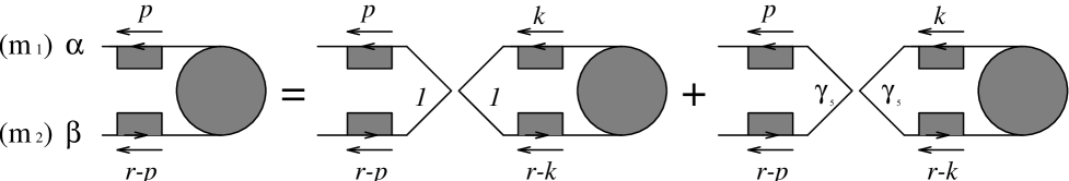
FIG. 1.: Bound state equation for the fermion–antifermion system in the Gross–Neveu model

Using the full propagator, we may straightforwardly obtain the Bethe–Salpeter equation for what we shall call the “meson wavefunction”, $\tilde{\psi}_{\alpha\beta}$, from the contributions graphically represented in fig. 1 as:

$$\tilde{\psi}_{\alpha\beta}(p,r)=2a_{b}^{2}N\left[S_{\alpha 1}(p)S_{1\beta}(p-r)\int\!\!{d^{2}k\over(2\pi)^{2}}\,\tilde{\psi}_{22}(k,r)+S_{\alpha 2}(p)S_{2\beta}(p-r)\int\!\!{d^{2}k\over(2\pi)^{2}}\,\tilde{\psi}_{11}(k,r)\right]$$ (4)

$S(p)$ is the full fermion propagator in this model, which is none other than the tree–level propagator with the mass $m$ replaced by $M$. $a_{b}$ denotes the bare four fermi coupling. Following ’t Hooft, we integrate over one component of the momentum $p_{+}$ and define $\tilde{\varphi}_{\alpha\beta}\equiv\int dp_{+}\tilde{\psi}_{\alpha\beta}$. Then, after some computation, the equations for the meson wavefunction $\tilde{\psi}_{\alpha\beta}$ reduce to the following equations for the components:

$${2\pi\over a_{b}^{2}N}\left[\tilde{\mu}^{2}-{1\over x(1-x)}\right]\tilde{\varphi}_{11}(x) = -{1\over 2(1-x)}\left[\tilde{\mu}^{2}-{1\over x}+{1\over 1-x}\right]\int_{0}^{1}\!\!dy\,\tilde{\varphi}_{11}(y)$$ (6)

$$\qquad+{1\over x(1-x)}\int_{0}^{1}\!\!dy\,\tilde{\varphi}_{22}(y)$$

$${2\pi\over a_{b}^{2}N}\left[\tilde{\mu}^{2}-{1\over x(1-x)}\right]\tilde{\varphi}_{22}(x) = -{1\over 2x}\left[\tilde{\mu}^{2}+{1\over x}-{1\over 1-x}\right]\int_{0}^{1}\!\!dy\,\tilde{\varphi}_{22}(y)$$ (8)

$$\qquad+{1\over x(1-x)}\int_{0}^{1}\!\!dy\,\tilde{\varphi}_{11}(y)$$

$${2\pi\over a_{b}^{2}N}{M\over\sqrt{2}r_{-}}\left[\tilde{\mu}^{2}-{1\over x(1-x)}\right]\tilde{\varphi}_{12}(x) = {1\over 1-x}\int_{0}^{1}\!\!dy\,\tilde{\varphi}_{11}(y)-{1\over x}\int_{0}^{1}\!\!dy\,\tilde{\varphi}_{22}(y)$$ (9)

$${2\pi\over a_{b}^{2}N}{\sqrt{2}r_{-}\over M}\left[\tilde{\mu}^{2}-{1\over x(1-x)}\right]\tilde{\varphi}_{21}(x) = -{1\over 2x(1-x)}\left[\tilde{\mu}^{2}-{1\over x}+{1\over 1-x}\right]\int_{0}^{1}\!\!dy\,\tilde{\varphi}_{11}(y)$$ (11)

$$\qquad+{1\over 2x(1-x)}\left[\tilde{\mu}^{2}+{1\over x}-{1\over 1-x}\right]\int_{0}^{1}\!\!dy\,\tilde{\varphi}_{22}(y)$$

Here, we defined the momentum fraction of the incoming antifermion $x\equiv p_{-}/r_{-}$ and the mass squared of the bound state in units of the fermion mass squared as $\tilde{\mu}^{2}=2r_{+}r_{-}/M^{2}$. Without any loss of generality, we may define $\int dx\tilde{\varphi}_{11}=1,\ \int dx\tilde{\varphi}_{22}=C$, where $C$ is to be determined later. Then all the meson wavefunctions $\tilde{\varphi}_{\alpha\beta}$ may be solved algebraically using the equations (6) as follows. The consistency with the normalization of $\tilde{\varphi}_{11}$ requires that

$${4\pi\over a_{b}^{2}N}=\int_{0}^{1}\!dx\,{{\tilde{\mu}^{2}\over 2}-2C-2+{1\over 2x(1-x)}\over 1-\tilde{\mu}^{2}x(1-x)}$$ (12)

The compatibility of this with the normalization condition for $\tilde{\varphi}_{22}$ requires that $C=\mp 1$. These two cases correspond to the meson states $\chi$ and $\sigma$ respectively. We obtain the equations determining the masses of $\chi$ and $\sigma$ as

$$\chi:\qquad{4\pi\over a^{2}N}=\int_{0}^{1}\!\!\!dx\,{\tilde{\mu}^{2}_{\chi}\over 1-\tilde{\mu}_{\chi}^{2}x(1-x)},\qquad\sigma:\qquad{4\pi\over a^{2}N}=\int_{0}^{1}\!\!\!dx\,{\tilde{\mu}^{2}_{\sigma}-4\over 1-\tilde{\mu}_{\sigma}^{2}x(1-x)}$$ (13)

Here, we renormalized the coupling constant as

$${4\pi\over a^{2}N}={4\pi\over a_{b}^{2}N}-{1\over 2}\int_{0}^{1}\!\!\!dx\,{1\over x(1-x)}$$ (14)

The integral needs to be regularized at the endpoints $0,1$ which is not explicitly expressed here. The same renormalization was employed in the light front Hamiltonian approach in [5]. This regularization is effectively an ultraviolet cutoff, which will become clear below. The meson wavefunctions for $\chi,\sigma$ can also be obtained algebraically as

$$\chi:\qquad\tilde{\varphi}_{12}^{\chi}(x)={\rm const.}\times{1\over 1-\tilde{\mu}_{\chi}^{2}x(1-x)},\qquad\sigma:\qquad\tilde{\varphi}_{12}^{\sigma}(x)={\rm const.}\times{1-2x\over 1-\tilde{\mu}_{\sigma}^{2}x(1-x)}$$ (15)

The component $\tilde{\varphi}_{12}$ is shown here since it corresponds to the relevant component of the meson wavefunction in the ’t Hooft model [1] and will also be the essential component in our analysis of the gauged four fermi model. The wavefunction for $\chi$ is consistent with the results obtained using light front Hamiltonian methods [6, 5]. Other components of the wavefunction can also be computed algebraically using (6).

B The analysis of the Gross–Neveu model using scalars and its relation to the Bethe–Salpeter equation

In this section, we clarify the relation between the results obtained above using the Bethe–Salpeter equation and the results obtained from using the auxiliary scalar fields $\sigma,\chi$ as in the Lagrangian (2). Since the approach of using scalars is more standard and is explained elsewhere, we refer the derivation to the literature [2, 3].

The full propagators for the $\sigma,\chi$ fields are [2]

$$\sigma:\qquad D^{-1}_{\sigma}(p^{2}) = 1+{a_{b}^{2}N\over 2\pi}\left[\ln{M^{2}\over\Lambda^{2}}+B(p^{2},M^{2})\right]$$ (16)

$$\chi:\qquad D^{-1}_{\chi}(p^{2}) = 1+{a_{b}^{2}N\over 2\pi}\left[\ln{M^{2}\over\Lambda^{2}}+{1\over 1-4M^{2}/p^{2}}B(p^{2},M^{2})\right]$$ (17)

where the $a_{b}$ is the bare coupling and $\Lambda$ is the ultraviolet momentum scale cutoff. (There is a mild abuse of notation here; this bare coupling is in principle not the same as the one in the previous section since the regularization methods are different.) The function $B(p^{2},M^{2})$ is defined as

$$B(p^{2},M^{2})\equiv\sqrt{1-4M^{2}/p^{2}}\ln{\sqrt{1-4M^{2}/p^{2}}+1\over\sqrt{1-4M^{2}/p^{2}}-1}=2\sqrt{4M^{2}/p^{2}-1}\cot^{-1}\sqrt{4M^{2}/p^{2}-1}$$ (18)

The renormalized coupling $a$ defined in (14) is related to the bare coupling $a_{b}$ here as

$${2\pi\over a^{2}N}={2\pi\over a_{b}^{2}N}+\ln{M^{2}\over\Lambda^{2}}$$ (19)

We find that the equations for the poles in the propagators for $\sigma,\chi$ in (16) indeed agree with the equations (13) in this renormalization scheme. The propagators have cuts for $p^{2}>4M^{2}$ corresponding to the production of physical fermion–antifermion pair of mass $M$ each.

The effective potential for the scalars may be obtained by computing the contributions from the fermion loops in the large–$N$ limit as

$$V(\sigma,\chi)={1\over 2}\left(\sigma^{2}+\chi^{2}\right)-{m\over a_{b}}\sigma+{a_{b}^{2}N\over 4\pi}\left(\sigma^{2}+\chi^{2}\right)\left(\ln{a_{b}^{2}\left(\sigma^{2}+\chi^{2}\right)\over\Lambda^{2}}-1\right)$$ (20)

By minimizing the potential, we obtain a vacuum expectation value $\langle\sigma\rangle$ for $\sigma$. The physical mass is related to the vacuum expectation value simply as $M=a_{b}\langle\sigma\rangle$, without loss of generality. We obtain a relation between the bare and the renormalized parameters

$${M\over a^{2}N}={m\over a_{b}^{2}N}$$ (21)

Since the mass is dynamically generated in the Gross–Neveu model even when $m=0$, the chiral limit corresponds to $a^{2}N\rightarrow\infty$.

C Physics of the Gross–Neveu model

Here, we briefly summarize the physics of the Gross–Neveu model, in particular, emphasizing the salient features and its underlying physics which will be useful later on. The Lagrangian (1) has two parameters, $m$ and $a$. Due to dimensional transmutation, the model is determined essentially by only one parameter. We can solve the equations (13) or the pole equations of the propagators (16) to obtain the masses of the scalars $\sigma,\chi$. We plot the spectrum of $\sigma,\chi$ against the inverse coupling in fig. 2.

FIG. 2.: Mass squared of $\chi$ (solid) and $\sigma$ (dashed) in units of $M^{2}$ versus the inverse coupling $2\pi/(a^{2}N)$.

We understand the various regions in the coupling constant as follows:

1. $1/a^{2}N=0$: The chiral point. Here, the masses for $\sigma$ and $\chi$ are respectively $2M$ and zero. The wavefunction for $\chi$, $\tilde{\varphi}_{12}^{\chi}(x)$, is a constant in this limit, similarly to the ’t Hooft model. $\chi$ is the “Nambu–Goldstone” boson of the theory. Strictly speaking, Nambu–Goldstone boson does not exist in $(1+1)$ dimensions [8], yet it is well known that many physical aspects of the higher dimensional theories are also seen in $(1+1)$ dimensional theories, especially in the large $N$ limit. A similar massless boson bound state exists in the ’t Hooft model in the chiral limit.

   The status of the $\sigma$ particle is interesting; while the $\sigma$ particle is usually said to exist, its wavefunction $\tilde{\varphi}_{12}^{\sigma}(x)$ approaches const.$/(1-2x)$ and is singular in the limit $1/a^{2}N\rightarrow 0$. Physical decay into a fermion and an antifermion becomes kinematically allowed in this limit $\mu^{2}\rightarrow 4M^{2}$ and the singular behavior is due to this. Similar behavior is also seen for $\chi$ in the limit $\mu^{2}\rightarrow 4M^{2}$. The wavefunction is well behaved when $a^{2}N<0$, yet in this region, the vacuum is not physically stable, as explained below.

2. $a^{2}N>0$: This region is physically consistent. The mass of $\chi$ is between zero and $2M$. The meson wavefunction has a singular limit $\tilde{\varphi}_{12}^{\chi}\rightarrow$const.$\times(1-2x)^{-2}$ as $1/a^{2}N\rightarrow\infty$. The pole in the $\sigma$ propagator (13) that exists for $a^{2}N\leq 0$ ceases to exist in this regime and there is no bound state corresponding to $\sigma$. Poles corresponding to resonance states also do not exist, unlike the Gross–Neveu model in $(2+1)$–dimensions[3].

3. $a^{2}N\leq-\pi$: While $\sigma$ scalar has a finite mass, $\chi$ is tachyonic. From the potential, we may understand this as follows; we are at an unstable vacuum where the potential is locally a minimum in the $\sigma$ direction yet maximal in the $\chi$ direction. Choosing the physically sensible vacuum reduces this case to the previous physically consistent case.

4. $-\pi<a^{2}N<0$: We again have chosen an unstable vacuum. this vacuum is unstable in both $\sigma$ and $\chi$ directions so that both $\sigma,\chi$ are tachyonic. Had the correct vacuum been chosen, the theory reduces to the $a^{2}N>0$ case above.

We plot the potential for these various cases in fig. 3 along the plane $\chi=0$.

FIG. 3.: The potential for the massive Gross–Neveu model in the $\sigma$–plane. $a_{b}\sigma=M$ is the “vacuum” we choose. An example is given for the each of the four cases 1—4 explained in the text. The values chosen are $(2\pi)/a^{2}N=0,1,-1$ and $-3$, respectively. Vertical scale is in units of $NM^{2}/2\pi$.

III The gauged four fermi model

In this section, we analyze the gauged four fermi model. We obtain the Bethe–Salpeter equation for the fermion–antifermion bound states — which we shall call the “mesons” for obvious reasons — and perform the renormalization of the model. We further systematically solve the Bethe–Salpeter equation to obtain the masses and the wavefunctions of the meson states.

The Lagrangian of the gauged four fermi model we work with is

$${\cal L}=-\frac{1}{2}\,{\rm tr}\,\left(F_{{\mu}{\nu}}F^{{\mu}{\nu}}\right)+\sum_{f}{\overline{\psi}}_{f}(i{\hbox{{\it D}\kern-5.20004pt\raise 1.29167pt\hbox{/}}}-m_{f}){\psi}_{f}+\frac{a^{2}}{2}\sum_{(f,f^{\prime})}({\overline{\psi_{f^{\prime}}}}{\psi_{f}})({\overline{\psi_{f}}}{\psi_{f^{\prime}}})-\frac{a_{5}^{2}}{2}\sum_{(f,f^{\prime})}({\overline{\psi_{f^{\prime}}}}{\gamma}_{5}{\psi_{f}})({\overline{\psi_{f}}}{\gamma}_{5}{\psi_{f^{\prime}}})\qquad$$ (22)

The covariant derivative is defined as $D_{\mu}\equiv\partial_{\mu}-igA_{\mu}$, where $g$ is the gauge coupling constant. The color indices have been suppressed. Index $f$ denotes the “flavor” index and is included here since we shall consider bound states involving fermions of different masses. The motivations for such a generalization is obvious when we want to apply the model to more realistic situations. The Lagrangian generically respects the global flavor symmetry $\left[U(1)_{V}\right]^{N}$, which is enlarged to $SU(N)_{V}\times U(1)_{V}$ when all the fermion masses $m_{f}$ are the same. This symmetry is further enlarged to the chiral flavor symmetry $SU(N)_{L}\times U(1)_{L}\times SU(N)_{R}\times U(1)_{R}$ when all $m_{f}=0$. The Gross–Neveu model we dealt with in the previous section corresponds to the case when there is no gauge coupling, only a single flavor type and $a^{2}=a_{5}^{2}$.

A The equations describing the mesons

Below, we will derive Bethe–Salpeter equations for the fermion bound states by using methods similar to those of ’t Hooft [1]. The situation is intrinsically more complicated than that of ’t Hooft since the four fermi interactions mix the fermions of different chirality and the Bethe–Salpeter equation can no longer be straightforwardly reduced to a one dimensional equation. We fix the gauge to the light-cone gauge $A_{-}=A^{+}=0$. Light-cone gauge has the advantage that there are no gluon self-interactions in $(1+1)$ dimensions. We take the large $N$ limit by letting $N$ go to infinity keeping $g^{2}N,a^{2}N,a_{5}^{2}N$ fixed.

First, we obtain the full propagator self consistently from the Schwinger–Dyson equation. Diagrammatically, the equation may be expressed as in fig. 4 in the large $N$ limit.

FIG. 4.: The self consistent equation for the propagator in the gauged four fermi model

Solving the equation we obtain the full propagator $S(p;M_{f})$ as

$$S^{-1}(p;M_{f})=-i\left[\hbox{{\it p}\kern-4.79996pt\raise-1.29167pt\hbox{/}}-M_{f}+i\epsilon+\frac{g^{2}N}{2\pi}\left(\frac{sgn(p_{-})}{{\lambda}_{-}}-\frac{1}{p_{-}}\right)\gamma^{+}\right]$$ (23)

where $M_{f}$ is the mass parameter containing the quantum corrections, as in the previous section. We introduced a cutoff ${\lambda}_{-}$ for the infrared divergence in $p_{-}$ integral.

The bound state equation for fermion–antifermion bound state may be derived in the large $N$ limit, which is diagrammatically depicted in fig. 5.

FIG. 5.: The bound state equation for the fermion–antifermion system in the gauged four fermi model.

Denoting the wavefunction of the bound state as ${\psi}_{{\alpha}{\beta}}(p,r)$, the Bethe–Salpeter equation can be derived as the following matrix equation in the large $N$ limit

$${\psi}(p,r) = -i2g^{2}N\,S(p;M_{1})\gamma^{+}\int\!\!{d^{2}k\over(2\pi)^{2}}\,{\psi}(p+k,r)\gamma^{+}S(p-r;M_{2}){1\over k_{-}^{2}}$$ (24)

$$- i{a_{b}^{2}N}\,S(p;M_{1})S(p-r;M_{2})\int\!\!{d^{2}k\over(2\pi)^{2}}\,\,{\rm tr}\,{\psi}(k,r)$$ (25)

$$+ ia_{5b}^{2}NS(p;M_{1})\gamma_{5}S(p-r;M_{2})\int\!\!{d^{2}k\over(2\pi)^{2}}\,\,{\rm tr}\,\left(\gamma_{5}{\psi}(k,r)\right)$$ (26)

The suffix $b$ on the couplings indicates that these couplings are bare parameters. We define, as in the previous section, ${\varphi}_{{\alpha}{\beta}}(p_{-},r){\equiv}\int_{-\infty}^{\infty}dp_{+}{\psi}_{{\alpha}{\beta}}(p,r)$. Then the bound state equations may be obtained for the components as

$$\left({\mu}^{2}-\frac{2r_{-}}{{\lambda_{-}}}-\frac{{\beta}_{1}-1}{x}-\frac{{\beta}_{2}-1}{1-x}\right){\varphi}_{11}(x)$$ (27)

$$\quad=\frac{M_{2}}{\sqrt{2}r_{-}(1-x)}\left(\frac{2r_{-}}{{\lambda_{-}}}{\varphi}_{12}(x)+P\!\!\int_{0}^{1}dy\frac{{\varphi}_{12}(y)}{(x-y)^{2}}\right)$$ (28)

$$\qquad+\frac{a_{b}^{2}N}{2{\pi}}\frac{1}{4x(1-x)}\left[2\sqrt{{\beta}_{1}{\beta}_{2}}-x\left(\mu^{2}-\frac{2r_{-}}{\lambda_{-}}-\frac{\beta_{1}-1}{x}-\frac{-{\beta}_{2}-1}{1-x}\right)\right]\int_{0}^{1}dy[{\varphi}_{11}(y)+{\varphi}_{22}(y)]$$ (29)

$$\qquad-\frac{a_{5b}^{2}N}{2{\pi}}\frac{1}{4x(1-x)}\left[2\sqrt{{\beta}_{1}{\beta}_{2}}+x\left({\mu}^{2}-\frac{2r_{-}}{{\lambda_{-}}}-\frac{{\beta}_{1}-1}{x}-\frac{-{\beta}_{2}-1}{1-x}\right)\right]\int_{0}^{1}dy[{\varphi}_{11}(y)-{\varphi}_{22}(y)]$$ (30)

$$\left({\mu}^{2}-\frac{2r_{-}}{\lambda_{-}}-\frac{\beta_{1}-1}{x}-\frac{{\beta}_{2}-1}{1-x}\right){\varphi}_{22}(x)$$ (31)

$$\quad=-\frac{M_{1}}{\sqrt{2}r_{-}x}\left(\frac{2r_{-}}{\lambda_{-}}{\varphi}_{12}(x)+P\int_{0}^{1}\!\!dy\,\frac{{\varphi}_{12}(y)}{(x-y)^{2}}\right)$$ (32)

$$\qquad+\frac{a_{b}^{2}N}{2{\pi}}\frac{1}{4x(1-x)}\left[2\sqrt{{\beta}_{1}{\beta}_{2}}-(1-x)\left({\mu}^{2}-\frac{2r_{-}}{\lambda_{-}}-\frac{-{\beta}_{1}-1}{x}-\frac{{\beta}_{2}-1}{1-x}\right)\right]\int_{0}^{1}\!\!dy\,[{\varphi}_{11}(y)+{\varphi}_{22}(y)]$$ (33)

$$\qquad+\frac{a_{5b}^{2}N}{2{\pi}}\frac{1}{4x(1-x)}\left[2\sqrt{{\beta}_{1}{\beta}_{2}}+(1-x)\left({\mu}^{2}-\frac{2r_{-}}{\lambda_{-}}-\frac{-{\beta}_{1}-1}{x}-\frac{{\beta}_{2}-1}{1-x}\right)\right]\int_{0}^{1}\!\!dy\,[{\varphi}_{11}(y)-{\varphi}_{22}(y)]$$ (34)

$$\left({\mu}^{2}-\frac{{\beta}_{1}-1}{x}-\frac{{\beta}_{2}-1}{1-x}\right){\varphi}_{12}(x)$$ (35)

$$\qquad=-P\!\!\int_{0}^{1}dy\frac{{\varphi}_{12}(y)}{(x-y)^{2}}-\frac{M_{1}(1-x)-M_{2}x}{2\sqrt{2}x(1-x)}\frac{a_{b}^{2}r_{-}}{g^{2}}\int_{0}^{1}dy\left[{\varphi}_{11}(y)+{\varphi}_{22}(y)\right]$$ (36)

$$\qquad+\frac{M_{1}(1-x)+M_{2}x}{2\sqrt{2}x(1-x)}\frac{a_{5b}^{2}r_{-}}{g^{2}}\int_{0}^{1}dy\left[{\varphi}_{11}(y)-{\varphi}_{22}(y)\right]$$ (37)

$$\left({\mu}^{2}-\frac{2r_{-}}{\lambda_{-}}-\frac{{\beta}_{1}-1}{x}-\frac{{\beta}_{2}-1}{1-x}\right){\varphi}_{21}(x)$$ (38)

$$\qquad=\frac{M_{1}M_{2}}{2r_{-}^{2}x(1-x)}\left(\frac{2r_{-}}{\lambda_{-}}{\varphi}_{12}(x)+P\!\!\int_{0}^{1}dy\frac{{\varphi}_{12}(y)}{(x-y)^{2}}\right)$$ (39)

$$\qquad+\frac{a_{b}^{2}N}{2{\pi}}\frac{1}{4\sqrt{2}x(1-x)}\biggl{[}-\left({\mu}^{2}-\frac{2r_{-}}{{\lambda_{-}}}-\frac{{\beta}_{1}-1}{x}-\frac{-{\beta}_{2}-1}{1-x}\right){M_{1}\over r_{-}}$$ (40)

$$\qquad\quad+\left({\mu}^{2}-\frac{2r_{-}}{\lambda_{-}}-\frac{-\beta_{1}-1}{x}-\frac{{\beta}_{2}-1}{1-x}\right){M_{2}\over r_{-}}\biggr{]}\int_{0}^{1}\!\!dy\,\left[{\varphi}_{11}(y)+{\varphi}_{22}(y)\right]$$ (41)

$$\qquad-\frac{a_{5b}^{2}N}{2{\pi}}\frac{1}{4\sqrt{2}x(1-x)}\biggl{[}\left({\mu}^{2}-\frac{2r_{-}}{{\lambda_{-}}}-\frac{{\beta}_{1}-1}{x}-\frac{-{\beta}_{2}-1}{1-x}\right){M_{1}\over r_{-}}$$ (42)

$$\qquad\quad+\left({\mu}^{2}-\frac{2r_{-}}{{\lambda_{-}}}-\frac{-{\beta}_{1}-1}{x}-\frac{{\beta}_{2}-1}{1-x}\right){M_{2}\over r_{-}}\biggr{]}\int_{0}^{1}\!\!dy\,\left[{\varphi}_{11}(y)-{\varphi}_{22}(y)\right]$$ (43)

Here we defined

$$\beta_{i}\equiv\pi{M^{2}_{i}\over g^{2}N},\quad\mu^{2}\equiv{\pi 2r_{+}r_{-}\over g^{2}N},\quad x\equiv\frac{p_{-}}{r_{-}},\quad y\equiv\frac{k_{-}}{r_{-}}$$ (44)

and $P\!\!\int$ denotes the principal part integral. When the four fermi couplings $a^{2},a_{5}^{2}$ are absent, the equation (35) is the ’t Hooft equation, which is a closed equation by itself. Here, all the equations are coupled and they need to be disentangled in a more sophisticated manner.

Superficially, we have as many equation as the unknowns — the meson wavefunctions, $\varphi_{\alpha\beta}$’s. However, we expect the infrared cutoff $\lambda_{-}$ to decouple from these physical equations, so that these equations are possibly over–constrained. It may be shown that all these equations consistently reduce to the following equations (45)—(48) and (35). These equations do not involve the infrared cutoff but are yet to be renormalized:

$${\varphi}_{11}(x)=\frac{-M_{2}}{\sqrt{2}r_{-}(1-x)}{\varphi}_{12}(x) - \frac{1}{4(1-x)}\frac{a_{b}^{2}N}{2\pi}\int_{0}^{1}dy[{\varphi}_{11}(y)+{\varphi}_{22}(y)]$$ (45)

$$- \frac{1}{4(1-x)}\frac{a_{5b}^{2}N}{2\pi}\int_{0}^{1}dy[{\varphi}_{11}(y)-{\varphi}_{22}(y)]$$ (46)

$${\varphi}_{22}(x)=\frac{M_{1}}{\sqrt{2}r_{-}x}{\varphi}_{12}(x)-\frac{a_{b}^{2}N}{2\pi}\frac{1}{4x}\int_{0}^{1}\!\!dy\,[{\varphi}_{11}(y)+{\varphi}_{22}(y)]+\frac{a_{5b}^{2}N}{2\pi}\frac{1}{4x}\int_{0}^{1}\!\!dy\,[{\varphi}_{11}(y)-{\varphi}_{22}(y)]$$ (47)

$${\varphi}_{21}(x)=-\frac{M_{1}M_{2}}{2r_{-}^{2}x(1-x)}{\varphi}_{12}(x) - \frac{M_{1}-M_{2}}{4\sqrt{2}r_{-}x(1-x)}\frac{a_{b}^{2}N}{2\pi}\int_{0}^{1}dy[{\varphi}_{11}(y)+{\varphi}_{22}(y)]$$ (48)

$$- \frac{M_{1}+M_{2}}{4\sqrt{2}r_{-}x(1-x)}\frac{a_{5b}^{2}N}{2\pi}\int_{0}^{1}dy[{\varphi}_{11}(y)-{\varphi}_{22}(y)]$$ (49)

From these equations we may derive the following closed equation for $\varphi_{12}(\equiv\varphi)$, whose suffix we shall omit for brevity from now on.

$${\mu}^{2}{\varphi}(x) \equiv H\varphi(x)$$ (50)

$$= \left(\frac{{\beta}_{1}-1}{x}+\frac{{\beta}_{2}-1}{1-x}\right){\varphi}(x)-P\int_{0}^{1}dy\frac{{\varphi}(y)}{(x-y)^{2}}$$ (53)

$$\quad-\frac{\sqrt{{\beta}_{1}}(1-x)-{\sqrt{{\beta}_{2}}}x}{x(1-x)}\frac{\int_{0}^{1}dy\frac{{\sqrt{{\beta}_{1}}}(1-y)-{\sqrt{{\beta}_{2}}}y}{y(1-y)}{\varphi}(y)}{\frac{4\pi}{a_{b}^{2}N}+\frac{1}{2}\int_{0}^{1}\frac{dx}{x(1-x)}}$$

$$\quad-\frac{\sqrt{{\beta}_{1}}(1-x)+{\sqrt{{\beta}_{2}}}x}{x(1-x)}\frac{\int_{0}^{1}dy\frac{{\sqrt{{\beta}_{1}}}(1-y)+{\sqrt{{\beta}_{2}}}y}{y(1-y)}{\varphi}(y)}{\frac{4\pi}{a_{5b}^{2}N}+\frac{1}{2}\int_{0}^{1}\frac{dx}{x(1-x)}}$$

We shall often refer to $H$ as the Hamiltonian. It is clear that this equation reduces to the ’t  Hooft equation when $a^{2}=a_{5}^{2}=0$ and that it reduces to the Gross–Neveu model case obtained in the previous section when $g=0$, $\beta_{1}=\beta_{2}$ and $a^{2}=a_{5}^{2}$. Even when the gauge coupling is zero, this model is more general than the massive Gross–Neveu model in that it incorporates different four fermi couplings $a,a_{5}$ and fermions of different masses. This equation describes the properties of the mesons in the gauged four fermi model. When the fermion masses are equal, ${\beta}_{1}={\beta}_{2}({\equiv}{\beta})$, the equation takes a substantially simpler form;

$${\mu}^{2}{\varphi}(x) = \frac{{\beta}-1}{x(1-x)}{\varphi}(x)-P\int_{0}^{1}dy\frac{{\varphi}(y)}{(x-y)^{2}}$$ (55)

$$\quad-\frac{{\beta}}{x(1-x)}\frac{\int_{0}^{1}dy\frac{{\varphi}(y)}{y(1-y)}}{\frac{4\pi}{a_{b}^{2}N}+\frac{1}{2}\int_{0}^{1}\frac{dx}{x(1-x)}}-\frac{{\beta}(1-2x)}{x(1-x)}\frac{\int_{0}^{1}dy\frac{1-2y}{y(1-y)}{\varphi}(y)}{\frac{4\pi}{a_{5b}^{2}N}+\frac{1}{2}\int_{0}^{1}\frac{dx}{x(1-x)}}$$

When the fermion masses are equal, $\beta_{1}=\beta_{2}$, and when the couplings are equal, $a^{2}=a_{5}^{2}$, the bound state equation for the mesons in the gauged four fermi model (50) reduces to the equation given by Burkardt [5]. Burkardt obtained a renormalized form of the equation when the meson wavefunction is an even function of the momentum fraction by using an operator identity involving the divergence of the axial current. In contrast, below, we will renormalize the more general bound state equation (50) and reduce the equations to its renormalized form without using any further identities.

B Renormalization of the gauged four fermi model

The equations derived in the previous section (45)–(50) are expressed in terms of bare quantities. The equation for the meson wavefunction should be expressible in terms of renormalized quantities and the Hamiltonian matrix elements between physical states should be finite. From these conditions, we may derive the renormalization for the couplings and the boundary conditions for the meson wavefunction. The coupling constants are renormalized as follows

$${4\pi\over a^{2}N}={4\pi\over a_{b}^{2}N}-{1\over 2}\int_{0}^{1}\!\!\!dx\,{1\over x(1-x)},\qquad{4\pi\over a_{5}^{2}N}={4\pi\over a_{5b}^{2}N}-{1\over 2}\int_{0}^{1}\!\!\!dx\,{1\over x(1-x)}$$ (56)

As in the Gross–Neveu model, these integrals have been regularized which is not explicitly denoted here. It should be noted here that this generalizes the renormalization of the coupling constant in the Gross–Neveu model (14). The mass parameter $M$ needs no renormalization. This is again consistent with the renormalization in both the Gross–Neveu model and the ’t Hooft model. We expand the meson wavefunction as

$$\varphi(x)=\varphi^{(0)}+\varphi^{(1)}(1-2x)+\hat{\varphi}(x)$$ (57)

where $\varphi^{(0)},\varphi^{(1)}$ are constants and $\hat{\varphi}(x)/\left[x(1-x)\right]$ is integrable at $x=0,1$. Then, the boundary conditions for the meson wavefunction are

$$\pmatrix{b_{+}&(1+4{a^{2}N\over 4\pi})b_{-}\cr b_{-}&(1+4{a_{5}^{2}N\over 4\pi})b_{+}\cr}\pmatrix{\varphi^{(0)}\cr\varphi^{(1)}\cr}=\int_{0}^{1}\!\!\!dx\,{\hat{\varphi}(x)\over x(1-x)}\pmatrix{{a^{2}N\over 4\pi}&0\cr 0&{a_{5}^{2}N\over 4\pi}\cr}\pmatrix{b_{+}&b_{-}\cr b_{-}&b_{+}\cr}\pmatrix{1\cr 1-2x\cr}$$ (58)

Here, we defined $b_{\pm}\equiv\left(\sqrt{\beta}_{1}\pm\sqrt{\beta}_{2}\right)/2$. In particular, when the coupling constants are equal, $a^{2}=a_{5}^{2}$, or when the masses are equal, $\beta_{1}=\beta_{2}$, the boundary conditions simplify to

$$\pmatrix{\varphi^{(0)}\cr\varphi^{(1)}\cr}=\int_{0}^{1}\!\!\!dx\,{\hat{\varphi}(x)\over x(1-x)}\pmatrix{{a^{2}N\over 4\pi}\cr{{a_{5}^{2}N\over 4\pi}(1-2x)\over 1+4{a_{5}^{2}N\over 4\pi}}\cr}$$ (59)

The meson wavefunction does not vanish at the boundaries. This property is similar to that of the Gross–Neveu model but unlike that of the ’t Hooft model. When the Gross–Neveu couplings are zero, the wavefunction does vanish at the boundaries, thereby recovering the boundary conditions of ’t Hooft. Also, it is instructive to check that the equation for the meson wavefunction (50) and the boundary conditions (59) for $\beta_{1}=\beta_{2}$ reduce exactly to the equations (13) in the Gross–Neveu model for $\sigma$ and $\chi$ scalars when $\varphi^{(0)}=0$ and $\varphi^{(1)}=0$, respectively.

The equation for the meson states is now reduced to

$$H\varphi(x) = \mu^{2}\varphi(x)$$ (60)

$$= \left({\beta_{1}-1\over x}+{\beta_{2}-1\over 1-x}\right)\hat{\varphi}(x)-P\!\!\int_{0}^{1}\!\!dy\,{\hat{\varphi}(y)\over(y-x)^{2}}+2\varphi^{(1)}\left(-\beta_{1}+\beta_{2}+\ln{1-x\over x}\right)$$ (61)

subject to the boundary conditions (58). It is straightforward to check that the Hamiltonian is Hermitean under the given boundary condition. The explicit dependence on the coupling constants is contained in the non–trivial boundary conditions. The problem has been reduced to that of solving a well defined integral equation. Below, we restrict to the case of scalar and pseudo scalar couplings being equal, $a=a_{5}$, for simplicity. We will, however, consider fermions of different masses in general. The more general case may be dealt with in a similar fashion, involving somewhat more complicated formulas. From here on, we shall use the notation $G\equiv a^{2}N/(4\pi)$ to avoid cluttering the formulas. For the case $a=a_{5}$, the matrix elements of the Hamiltonian may be simplified to the following form which is appropriate for the application of variational methods.

$$\left(\varphi^{\prime},H\varphi\right) = {1\over 2G}\left(\beta_{1}+\beta_{2}\right)\overline{\varphi^{\prime(0)}}\varphi^{(0)}+\left[{1+4G\over 2G}\left(\beta_{1}+\beta_{2}\right)+2\right]\overline{\varphi^{\prime(1)}}\varphi^{(1)}$$ (66)

$$\quad+2\int_{0}^{1}\!\!\!dx\,\ln{1-x\over x}\left(\overline{\hat{\varphi}^{\prime}(x)}\varphi^{(1)}+\overline{\varphi^{\prime(1)}}\hat{\varphi}(x)\right)$$

$$\quad+\left({\beta_{1}+\beta_{2}\over 2}-1\right)\int_{0}^{1}\!\!\!dx\,{\overline{\hat{\varphi}^{\prime}(x)}\hat{\varphi}(x)\over x(1-x)}-P\!\!\int_{0}^{1}\int_{0}^{1}\!\!{dx\,dy\over(y-x)^{2}}\,\overline{\hat{\varphi}^{\prime}(x)}\hat{\varphi}(y)$$

$$\quad+{1\over 2}\left(\beta_{1}-\beta_{2}\right)\biggl{[}{1\over G}\left(\overline{\varphi^{\prime(1)}}\varphi^{(0)}+\overline{\varphi^{\prime(0)}}\varphi^{(1)}\right)-4\int_{0}^{1}\!\!\!dx\,\left(\overline{\hat{\varphi}^{\prime}(x)}\varphi^{(1)}+\overline{\varphi^{\prime(1)}}\hat{\varphi}(x)\right)$$

$$\qquad\quad+\int_{0}^{1}\!\!\!dx\,{(1-2x)\overline{\hat{\varphi}^{\prime}(x)}\hat{\varphi}(x)\over x(1-x)}\biggr{]}$$

IV Systematic methods for solving the meson bound state equation

In this section, we show how the meson bound state equation (50) may be solved systematically utilizing a finite dimensional system of algebraic equations. We will give explicit formulas for two approaches, namely a variational method using polynomials of the momentum fraction and a method of working with the equation directly using a sinusoidal basis. These methods will be used in the next section to investigate some physical properties of the gauged four fermi model.

A Variational method

Here, we shall use a variational method using polynomials of the momentum fraction $x$ that satisfy the boundary condition (58). In the ’t Hooft model, a similar method was employed in [9]. Without loss of generality, the basis may be chosen to be

$$\varphi_{2k}(x)=G+{\left[x(1-x)\right]^{k}\over B(k,k)},\qquad\varphi_{2k+1}(x)=(1-2x)\left({G\over 1+4G}+{(2k+1)\left[x(1-x)\right]^{k}\over B(k,k)}\right),\qquad k=1,2,\ldots$$ (67)

The normalization factor was chosen so as to make the matrix elements be of order one. The meson bound state equation becomes

$$\det({\mu}^{2}N_{kl}-H_{kl})=0,\quad H_{kl}\equiv\left(\varphi_{k},H\varphi_{l}\right),\ N_{kl}\equiv\left(\varphi_{k},\varphi_{l}\right)\qquad k,l=2,3,4{\ldots}$$ (68)

In practice, we approximate the solution by using a finite dimensional version of this equation. The matrix elements can be computed to be

$$H_{2k,2l} = {1\over 2}\left(\beta_{1}+\beta_{2}-2\right){B(k+l,k+l)\over B(k,k)B(l,l)}+{G\over 2}\left(\beta_{1}+\beta_{2}\right)+{kl\over 2(k+l)}$$ (69)

$$H_{2k+1,2l+1} = {1\over 2}\left(\beta_{1}+\beta_{2}-2\right){(2k+1)(2l+1)B(k+l,k+l)\over(2k+2l+1)B(k,k)B(l,l)}+{G\over 2(1+4G)}\left(\beta_{1}+\beta_{2}\right)$$ (71)

$$\quad+2\left({G\over 1+4G}\right)^{2}+{G\over 1+4G}\left({k\over k+1}+{l\over l+1}\right)+{kl(2k+1)(2l+1)\over 2(k+l)(k+l+1)}$$

$$H_{2k,2l+1} = H_{2l+1,2k}={1\over 2}\left(\beta_{1}-\beta_{2}\right)\left[{G\over 1+4G}{1\over 2k+1}+{(2l+1)B(k+l,k+l)\over(2k+2l+1)B(k,k)B(l,l)}\right]$$ (72)

$$N_{2k,2l} = {(k+l)B(k+l,k+l)\over 2(2k+2l+1)B(k,k)B(l,l)}+G^{2}+G\left[{k\over 2(2k+1)}+{l\over 2(2l+1)}\right]$$ (73)

$$N_{2k+1,2l+1} = {(2k+1)(2l+1)(k+l)B(k+l,k+l)\over 2(2k+2l+3)(2k+2l+1)B(k,k)B(l,l)}+{1\over 3}\left({G\over 1+4G}\right)^{2}$$ (75)

$$\qquad+{G\over 2(1+4G)}\left({k\over 2k+3}+{l\over 2l+3}\right)$$

$$N_{2k,2l+1} = N_{2k+1,2l}=0$$ (76)

When the fermion masses are equal, $\beta_{1}=\beta_{2}$, the even and the odd sectors decouple.

B Multhopp’s method

Rather than using a variational method, we may choose to work with the equation (60) directly. By a clever choice of basis, this singular integral equation may be brought into an algebraic equation. The method we use here generalizes the methods used to numerically analyze the ’t Hooft equation previously [10, 7].

We expand the meson wavefunction as

$$\varphi(x)=\varphi^{(0)}-\varphi^{(1)}\cos\theta+\sum c_{n}\sin n\theta,\qquad x\equiv{1\over 2}(1+\cos\theta)$$ (77)

$\varphi^{(0,1)}$ terms are absent in the ’t Hooft equation and can be determined in our model from the boundary conditions (58).

$$\varphi^{(0)}=2\pi G\sum_{n:\ \rm odd}c_{n},\qquad\varphi^{(1)}=-2\pi{G\over 1+4G}\sum_{n:\ \rm even}c_{n},\qquad$$ (78)

then the meson equation (60) becomes

$$\sum_{n}\left[\mu^{2}\hat{P}_{n}(\theta)-\hat{M}_{n}(\theta)\right]c_{n}=0$$ (79)

where

$$\hat{P}_{n}(\theta) \equiv \sin n\theta+2\pi\cases{G&$n$: odd\cr{G\over 1+4G}\cos\theta&$n$: even\cr}$$ (80)

$$\hat{M}_{n}(\theta) \equiv 2\left({\beta_{1}-1\over 1+\cos\theta}+{\beta_{2}-1\over 1-\cos\theta}\right)\sin n\theta+2\pi{n\sin n\theta\over\sin\theta}+\cases{0&$n$: odd\cr 4\pi{G\over 1+4G}\left(\beta_{1}-\beta_{2}+\ln{1+\cos\theta\over 1-\cos\theta}\right)&$n$: even\cr}$$ (81)

In practice, we truncate the basis to a finite dimensional one and systematically analyze the convergence of the solution by varying the dimension of this finite space, which we shall denote by $K$. Then the meson bound state equation may be reduced to a generalized eigenvalue problem.

$$\sum_{n=1}^{K}\left[\mu^{2}P_{mn}-M_{mn}\right]c_{n}=0$$ (82)

where

$$P_{mn}\equiv\sum_{l=1}^{K}g_{m}(\theta_{l})\hat{P}_{n}(\theta_{l}),\quad M_{mn}\equiv\sum_{l=1}^{K}g_{m}(\theta_{l})\hat{M}_{n}(\theta_{l}),\qquad\theta_{j}\equiv\pi{j\over K+1}$$ (83)

In this work, we choose $g_{m}(\theta)=2\sin m\theta/(K+1)$ as in the ’t Hooft model. Other choices may be more convenient depending on the parameters of the model. Similarly to the variational method given above, $M_{mn},P_{mn}\propto\left(\beta_{1}-\beta_{2}\right)$ when $m-n\equiv 1\ ({\rm mod}\ 2)$ and the even and odd sectors decouple completely when $\beta_{1}=\beta_{2}$. This property is preserved for any choice of $g_{m}(\theta_{l})$ as long as the property $g_{m}(\theta_{l})=(-1)^{m+1}g_{m}(\theta_{K+1-l})$ is preserved. Unlike the variational method, however, the approximate solution obtained by truncating to finite dimensional solution space needs not be an upper bound on the true solution and in general will not be.

V Physics of the gauged four fermi model

First, we would like to determine the parameter region where the behavior of the system is physically reasonable. In particular, the meson bound state should not be tachyonic. Here, we will perform the analysis for fermions of equal mass since we expect tachyonic mesons in the flavor singlet channel if tachyonic mesons exist at all. Using the variational method for the meson wavefunction in a manner similar to the previous section,

$$\varphi_{\gamma}(x)\equiv G+B(\gamma,\gamma)^{-1}\left[x(1-x)\right]^{\gamma}\qquad\gamma>0$$ (84)

we obtain an upper bound $\mu^{2}_{\gamma}$ for the meson mass squared for each $\gamma>0$.

$$\mu^{2}_{\gamma}={\left(\varphi_{\gamma},H\varphi_{\gamma}\right)\over\left(\varphi_{\gamma},\varphi_{\gamma}\right)}={G\beta+{\gamma\over 4}+(\beta-1){B(2\gamma,2\gamma)\over B(\gamma,\gamma)^{2}}\over G^{2}+G{\gamma\over 2\gamma+1}+{\gamma\over 4\gamma+1}{B(2\gamma,2\gamma)\over B(\gamma,\gamma)^{2}}}\sim\cases{{\beta\over G}&$\gamma\sim 0$\cr 2\sqrt{2\pi\gamma}&$\gamma\sim\infty$\cr}$$ (85)

This immediately establishes that when $\beta G<0$ tachyonic mesons will appear. While it is logically possible from this analysis that the region with both $\beta<0$ and $G<0$ may be physically consistent, it is unreasonable to expect so; in practice, we find that tachyonic mesons appear for this case also, when we have a large enough variational space. Therefore, we henceforth interest ourselves in the region $G>0$ and $\beta>0$.

Using the methods explained in the previous section, we may obtain the spectrum and the meson wavefunctions. We plot the spectrum and the wave functions for some typical cases below in figures fig. 6, fig. 7 and fig. 8. We have added a brief note on the convergence of the numerical data as an appendix.

FIG. 6.: Mass squared of the lightest four meson states versus the coupling $G$ for $\beta=1$.

FIG. 7.: Mass squared of the lightest four meson states versus the fermion mass squared $\beta$ for the coupling $G=1$.

FIG. 8.: The meson wavefunctions for the gauged four fermi model (solid), the ’t Hooft model (long dashes) and the Gross–Neveu model (short dashes). The functions are plotted for the lightest two meson states. The parameters chosen for the gauged four fermi model is $G=1,\beta=1$ for both mesons. For the ’t Hooft model $\beta=1$ also. For the Gross–Neveu model, in the lightest meson case, the meson mass was chosen to agree with that of the gauged four fermi model. In the next lightest meson case, $\mu^{2}/\beta=3$ was chosen.

As in the ’t Hooft model, the fermions are confined and the following Regge–type behavior is observed for the highly massive mesons, similarly to the ’t Hooft model:

$$\mu^{2}\sim\pi^{2}k\qquad k\gg 1,\ \beta$$ (86)

This Regge behavior is shown in fig. 9.

FIG. 9.: Mass squared normalized by $\pi^{2}$ of the meson states versus the “level number” for the case $\beta=1$, $G=1$. $\Box$ ($+$)’s denote states whose wavefunctions are even (odd) under $x\leftrightarrow 1-x$,

We may understand the behavior of the spectrum in the various limits of the model as follows: when we turn off the Gross–Neveu coupling $a^{2}$, the spectrum reduces to that of the ’t  Hooft model. As we take the gauge coupling to zero, which effectively is the limit $\beta\rightarrow\infty$, the splitting between the higher levels disappear. We have explicitly checked that the mass of the lightest meson approaches to the Gross–Neveu model value plotted in fig. 2 in this limit. For the higher levels, $\mu^{2}$ approaches $4\beta$ in this Gross–Neveu limit. The chiral limit may be identified as the limit $G\ ({\rm or}\ a^{2}N)\rightarrow\infty$, similarly to the Gross–Neveu model case. In the spectrum, mass of the meson states decrease as we approach the chiral limit and it is clear that $\mu^{2}\rightarrow 0$ for the lightest meson bound state in the limit $G\rightarrow\infty$. When the limit $\beta\rightarrow\infty$ is taken in addition, it may be explicitly checked that the next lightest meson satisfies $\mu^{2}/M^{2}\rightarrow 4$ corresponding the the $\sigma$ mass in the Gross–Neveu model.

As $\beta$ becomes large, the meson masses behave linearly with the quark masses, as is expected from the naive constituent quark picture. This picture is supposedly valid for highly massive quarks. The lightest meson behaves in a qualitatively different manner from the other meson states in the theory. This is a feature of the gauged four fermi model; such a behavior does not occur in the ’t Hooft model. The Gross–Neveu coupling affects the lightest meson state relatively more than the other meson states. This disparate behavior is a necessary consequence of the Gross–Neveu limit where $\mu^{2}/\beta$ of $\chi$ and the other mesons approach the corresponding value $\tilde{\mu}^{2}$ in the Gross–Neveu model and four. In the ’t Hooft model, $\mu^{2}/\beta$ for the lightest meson also approaches four for large $\beta$.

VI Summary and discussions

In this work, we have solved the meson sector of the gauged four fermi model in the large $N$ limit. We provided detailed prescriptions for solving the model systematically which should be useful for further work involving this class of models. We also determined the physically consistent region in the gauged four fermi model and analyzed the model there. However, it is possible that the regions with tachyons correspond to other phases of the model that is inaccessible to our current methods.

Both the Gross–Neveu model and the ’t  Hooft model have been used extensively in the literature to understand the physical behavior of real systems, such as QCD. A model that combines the two models should be quite useful for understanding the dynamics of various field theories. In one direction, the four fermi coupling has been used to model strong interaction dynamics involving dynamical symmetry breaking for quite some time [11]. By interpolating between these two models, we intend to shed more light on the relation between the physical behavior of these two theories. Furthermore, when dynamical symmetry breaking scales are widely separated, in the intermediate energy range, the theory effectively becomes a gauged four fermi model. Such situations can occur quite generally where the lower energy scale is the QCD scale or some technicolor scale. These types of theories are of phenomenological interest and have been studied actively, for instance, in the so called “top quark condensation” models [12, 11]. Admittedly, the model we studied is a $(1+1)$ dimensional toy model version of such theories. Historically, however, $(1+1)$ dimensional theories have played an important role in understanding of the corresponding higher dimensional theories and we hope this will also be true in the future.

Acknowledgments: We would like to thank Tomoyasu Ichihara for his collaboration during the early stages of this work. We would also like to thank K. Itakura and H.  Sonoda for discussions.

Appendix: A brief note on the convergence of numerical solutions

The convergence of the numerical solutions depends on the parameters $(G,\beta)$. When $\beta\gtrsim 1$, it is relatively easy to achieve a relative accuracy of $\sim 10^{-4}$ in the meson mass at least using both the variational method (dimension $\sim 10$) and Multhopp’s method (dimension $\sim 400$). For $\beta\lesssim 1$, more effort is needed to achieve the same level of convergence. The difficulties in the variational method using polynomials of the momentum fraction (section IV A) arise because of the round off errors since the eigenvalues in the normalization matrix (73) tend to become small. Analytically choosing an orthonormal basis or using some other basis appropriate for the parameter region in question might alleviate this problem. In Multhopp’s method (section IV B), the limitations arise due to the necessary computational time when using larger space of functions. Choice of $g_{m}(\theta)$ may speed up the convergence process in some parameter regions.

In the parameter regions where the convergence is slow, extrapolation in the data can be effective. We have found that trial functions of the type $x+aK^{b}$ fits the data quite well. Here $x$ is the extrapolated value, $K$ is the dimension of the space span by the basis and $a,b$ are parameters. Extrapolation can sometimes be misleading so checks on the results are desirable. In our case, we compare the extrapolation values from both the variational method and Multhopp’s method and we confirm that they are consistent within the errors of the fit. An example of such an extrapolation is shown in fig. 10.

FIG. 10.: Extrapolation of the numerical data for the variational method and Multhopp’s method. In this example, $G=1$ and $\beta=0.1$ and $\mu^{2}=0.095\pm 0.002$.

REFERENCES

• [1] G. ’t Hooft, Nucl. Phys. B72 (1974) 461, Nucl. Phys. B75 (1974) 461
• [2] D.J. Gross, A. Neveu, Phys. Rev. D10 (1974) 3235
• [3] S. Coleman, “Aspects of symmetry”, Cambridge University Press (1985); B. Rosenstein, B.J. Warr, S.H. Park, Phys. Rep. C205 (1991) 59
• [4] N. Andrei, J.H. Lowenstein, Phys. Rev. Lett. 43 (1979) 1698; Phys. Lett. B90 (1980) 106
• [5] M. Burkardt, Phys. Rev. D56 (1997) 7105
• [6] K. Itakura, Ph D thesis, Tokyo University (1996)
• [7] K. Aoki, T. Ichihara, Phys. Rev. D52 (1995) 6435
• [8] S. Coleman, Comm. Math. Phys. 31 (1973) 259
• [9] W.A.  Bardeen, R.B. Pearson, E. Rabinovici, Phys. Rev. 21 (1980) 1037
• [10] A.J. Hanson, R.D. Peccei, M.K. Prasad, Nucl. Phys. B121 (1977) 477; R.C. Brower, W.L. Spence, J.H. Weis, Phys. Rev. 19D (1979) 3024; S. Huang, J.W. Negele, J. Polonyi, Nucl. Phys. B307 (1988) 669; R.L. Jaffe, P.F. Mende, Nucl. Phys. B369 (1992) 182
• [11] Y. Nambu, G. Jona-Lasinio Phys. Rev. 122 (1961) 345; For recent reviews, see for instance, J.L. Rosner, hep-ph/9812537, R.S. Chivukula, hep-ph/9903500.
• [12] Y. Nambu, in New Theories in Physics, Z. Ajduk, S. Pokorski, A. Trautman (eds), World Scientific, Singapore (1989); and in New Trends in Strong Coupling Gauge Theories, M. Bando, T. Muta, K. Yamawaki (eds), World Scientific, Singapore (1989); V.A. Miransky, M. Tanabashi, K. Yamawaki, Mod. Phys. Lett. A4 (1989) 1043; Phys. Lett. B221 (1989) 177; W.A. Bardeen, C.T. HIll, M. Lindner, Phys. Rev. D41 (1990) 1647