Constraints on the phase $\gamma$ and new physics from $B\to K\pi$ Decays

Abstract

Recent results from CLEO on $B\to K\pi$ indicate that the phase $\gamma$ may be substantially different from that obtained from other fit to the KM matrix elements in the Standard Model. We show that $\gamma$ extracted using $B\to K\pi,\pi\pi$ is sensitive to new physics occurring at loop level. It provides a powerful method to probe new physics in electroweak penguin interactions. Using effects due to anomalous gauge couplings as an example, we show that within the allowed ranges for these couplings information about $\gamma$ obtained from $B\to K\pi,\pi\pi$ can be very different from the Standard Model prediction.

The CLEO collaboration has recently measured the four $B\to K\pi$ branching ratios with[1], $Br(B^{\pm}\to\pi^{\pm}K^{0})=(1.82^{+0.46}_{-0.4}\pm 0.16)\times 10^{-5}$, $Br(B^{\pm}\to K^{\pm}\pi^{0})=(1.21^{+0.30+0.21}_{-0.28-0.14})\times 10^{-5}$, $Br(B\to K^{\pm}\pi^{\mp})=(1.88^{+0.28}_{-0.26}\pm 0.13)\times 10^{-5}$ and $Br(B\to K^{0}\pi^{0})=(1.48^{+0.59+0.24}_{-0.51-0.33})\times 10^{-5}$. It is suppressing that these branching ratios turn out to be close to each other because naive expectation of strong penguin dominance would give $R=Br(K^{\pm}\pi^{0})/Br(K\pi^{\pm})\sim 1/2$ and model calculations for $Br(B^{0}\to K^{0}\pi^{0})$ would obtain a much smaller value. The closeness of the branching ratios with charged mesons in the final states may be an indication of large interference effects of tree, strong and electroweak penguin interactions[2]. It has been shown that using information from these decays and $B^{\pm}\to\pi^{\pm}\pi^{0}$ decays, the phase angle $\gamma$ of the KM matrix can be constrained[3] and determined[4] in the Standard Model (SM). Using the present central values for these branching ratios we find that the constraint obtained on $\gamma$ may have potential problem with $\gamma=(59.5^{+8.5}_{-7.5})^{\circ}$ obtained from other constraints[5].

If there is new physics beyond the SM the situation becomes complicated[6, 7]. It is not possible to isolate different new physics sources in the most general case. However, one can extract important information for the class of models where significant new physics effects only show up at loop levels for B decays[6, 7]. In this paper we study how new physics of the type described above can affect the results using anomalous three gauge boson couplings as an example for illustration.

New physics due to anomalous three gauge boson couplings is a perfect example of models where new physics effects only appear at loop level in B decays. Effects due to anomalous couplings do not appear at tree level for B decays to the lowest order, and they do not affect CP violation and mixings in $K^{0}-\bar{K}^{0}$ and $B-\bar{B}$ systems at one loop level. Therefore they do not affect the fitting to the KM parameters obtained in Ref. [5]. However they affect the constraint on and determination of $\gamma$ using experimental results from $B\to K\pi,\pi\pi$, and affect the $B$ decay branching ratios.

The effective Hamiltonian $H_{eff}=(G_{F}/\sqrt{2})[V_{ub}^{*}V_{uq}(c_{1}O_{1}+c_{2}O_{2})-V_{tb}^{*}V_{tq}\sum_{i=3-10}c_{i}O_{i}]$ responsible for B decays have been studied by many authors[8]. We will use the values of $c_{i}$ obtained for the SM in Ref.[9] with

$$c_{1}=-0.313,\;\;c_{2}=1.150,\;\;c_{3}=0.017,\;\;c_{4}=-0.037,\;\;c_{5}=0.010,\;\;c_{6}=-0.046,$$ (1)

$$c_{7}=-0.001\alpha_{em},\;\;c_{8}=0.049\alpha_{em},\;\;c_{9}=-1.321\alpha_{em},\;\;c_{10}=0.267\alpha_{em}.$$ (2)

The Wilson Coefficients are modified when anomalous couplings are included. They will generate non-zero $c_{3-10}$[10]. Their effects on $B\to K\pi$ mainly come from $c_{7-10}$. To the leading order in QCD corrections, the new contributions to $c_{7-10}^{AC}$ due to various anomalous couplings are given by,

$$c^{AC}_{7}/\alpha_{em} = -0.287\Delta\kappa^{\gamma}-0.045\lambda^{\gamma}+1.397\Delta g_{1}^{Z}-0.145g_{5}^{Z},$$ (3)

$$c^{AC}_{8}/\alpha_{em} = -0.082\Delta\kappa^{\gamma}-0.013\lambda^{\gamma}+0.391\Delta g_{1}^{Z}-0.041g_{5}^{Z},$$ (4)

$$c^{AC}_{9}/\alpha_{em} = -0.337\Delta\kappa^{\gamma}-0.053\lambda^{\gamma}-5.651\Delta g_{1}^{Z}+0.586g_{5}^{Z},$$ (5)

$$c^{AC}_{10}/\alpha_{em} = 0.069\Delta\kappa^{\gamma}+0.011\lambda^{\gamma}+1.143\Delta g_{1}^{Z}-0.119g_{5}^{Z}.$$ (6)

In the above we have used a cut off $\Lambda=1$ TeV for terms proportional to $\Delta\kappa^{\gamma}$ and $\Delta g_{1}^{Z}$. Contributions from other anomalous couplings are suppressed by additional factors of order $(m_{b}^{2},m_{B}^{2})/m_{W}^{2}$ which can be safely neglected. There are constraints on the anomalous gauge couplings[11, 12]. LEP experiments obtain[12], $-0.217<\Delta\kappa^{\gamma}<0.223$, $-0.158<\lambda^{\gamma}<0.074$, and $-0.113<\Delta g_{1}^{Z}<0.126$ at the 95% confidence level. Assuming that $g_{5}^{Z}$ is the same order as $\Delta g_{1}^{Z}$, it is clear that the largest possible contribution may come from $\Delta g^{Z}_{1}$. In our later discussions we consider $\Delta g^{Z}_{1}$ effects only.

To see possible deviations from the SM predictions for $B\to K\pi$ data, we carried out a calculation using factorization following Ref. [13] with $V_{us}=0.2196$, $V_{cb}\approx-V_{ts}=0.0395$, $|V_{ub}|=0.08V_{cb}$[14]. The branching ratios as functions of $\gamma$ are shown in Fig. 1. In this figure we used $m_{s}=100$ MeV which is at the middle of the range from lattice calculations[15] and the number of colors $N_{c}=3$. Since penguin dominates the branching ratio for $Br(B^{+}\to K^{0}\pi^{+})$ which is insensitive to $\gamma$, we normalize the branching ratios to $Br(B^{+}\to K^{0}\pi^{+})$ to reduce possible uncertainties in the overall normalization of form factors involved.

From Fig. 1, we see that the central values for the branching ratios for the ones with at least one charged meson in the final states require the angle $\gamma$ to be within $75^{\circ}$ to $80^{\circ}$ rather than the best fit value $\gamma_{best}=59.5^{\circ}$ in Ref.[5]. Larger $\gamma$ is also indicated by other rare B decay data[16]. When effects due to $\Delta g^{Z}_{1}$ is included the situation can be relaxed. The effects of $\Delta g^{Z}_{1}$ on $B^{+}\to K^{0}\pi^{+},K^{+}\pi^{-}$ are very small, but are significant for $B^{+}\to K^{+}\pi^{0}$ and $B\to K^{0}\pi^{0}$. With positive $\Delta g^{Z}_{1}$ in its allowed range, it is possible for the relative ratios of $Br(B^{+}\to K^{+}\pi^{0})$ to the other charged modes to be in agreement with data for $\gamma=\gamma_{best}$. We note that $\Delta g^{Z}_{1}$ does not affect the ratio $Br(B^{0}\to K^{+}\pi^{-})/Br(B^{+}\to K^{0}\pi^{+})$. Its experimental value prefers $\gamma$ to be close to $75^{\circ}$. Of course we also note that this situation can be improved by treating $N_{c}$ as a free parameter to take into account certain non-factorizable effects. We find that with $N_{c}\approx 1.35$, the central experimental values for the branching ratios of B decays into charged mesons in the final states can be reproduced for $\gamma=\gamma_{best}$. It is not possible to bring $Br(B^{0}\to K^{0}\pi^{0})$ up to the experimental central value even with allowed $\Delta g^{Z}_{1}$ and reasonable values for $N_{c}$ and $m_{s}$.

If the present experimental central values will persist and factorization approximation with $N_{c}=3$ is valid, new physics may be needed. Needless to say that we have to wait for more accurate data to draw firmer conclusions. Also due to our inability to reliably calculate the hadronic matrix elements, one should be careful in drawing conclusions with factorization calculations. However, we would like to point out that data on rare B to $K\pi$ decays may provide a window to look for new physics beyond the SM. Of course, to have a better understanding of the situation one needs to find methods which are able to extract $\gamma$ in a model independent way and in the presence of new physics. In the following we will analyze some rare B to $K\pi$ decay data in a more model independent way.

Model independent constraint on $\gamma$ can be obtained using branching ratios for $B^{\pm}\to K\pi$ and $B^{\pm}\to\pi\pi$ from symmetry considerations. This method would only need information from charged B decays to $K\pi$ and $\pi\pi$, and therefore this method is not affected by the uncertainties associated with neutral B decays to $K\pi$ modes. Using SU(3) relation and factorization estimate for SU(3) breaking effect among $B^{\pm}\to K\pi$ and $B^{\pm}\to\pi\pi$, one obtains[3, 4]

$$A(\pi^{+}K^{0})+\sqrt{2}A(\pi^{0}K^{+})=\epsilon A(\pi^{+}K^{0})e^{i\Delta\phi}{e^{i\gamma}-\delta_{EW}\over 1-\delta_{EW}^{\prime}},$$ (7)

$$\delta_{EW}=-{3\over 2}{|V_{cb}||V_{cs}|\over|V_{ub}||V_{us}|}{c_{9}+c_{10}\over c_{1}+c_{2}},\;\;\;\;\delta_{EW}^{\prime}={3\over 2}{|V_{tb}||V_{td}|\over|V_{ub}||V_{ud}|}e^{i\alpha}{c_{9}+c_{10}\over c_{1}+c_{2}},$$ (8)

$$\epsilon=\sqrt{2}{|V_{us}|\over|V_{ud}|}{f_{K}\over f_{\pi}}{|A(\pi^{+}\pi^{0})|\over|A(\pi^{+}K^{0})|},$$ (9)

where $\Delta\phi$ is the difference of the final state elastic re-scattering phases $\phi_{3/2,1/2}$ for $I=3/2,1/2$ amplitudes. For $f_{K}/f_{\pi}=1.22$ and $Br(B^{\pm}\to\pi^{\pm}\pi^{0})=(0.54^{+0.21}_{-0.20}\pm 0.15)\times 10^{-5}$, we obtain $\epsilon=0.21\pm 0.06$.

The parameter $\delta_{EW}^{\prime}$ is of order $c_{9,10}/c_{1,2}$ which is much smaller than one and will be neglected in our later discussions. $\delta_{EW}$ is a true measure of electroweak penguin interactions in hadronic B decays and provides an easier probe of these interactions compared with other methods[17]. In the above contributions from $c_{7,8}$ have been neglected which is safe in the SM because they are small. With anomalous couplings this is still a good approximation. In general the contributions from $c_{7,8}$ may be substantial. In that case the expression becomes more complicated. But one can always absorb the contribution into an effective $\delta_{EW}$. In the SM for $r_{v}=|V_{ub}|/|V_{cb}|=0.08$ and $|V_{us}|=0.2196$[14], $\delta_{EW}=0.81$. Smaller $r_{v}$ implies larger $\delta_{EW}$. Had we used $r_{v}=0.1$, $\delta_{EW}$ would be 0.65 as in Ref. [3, 4]. With anomalous couplings, we find

$$\delta_{EW}=0.81(1+0.26\Delta\kappa^{\gamma}+0.04\lambda^{\gamma}+4.33\Delta g_{1}^{Z}-0.45g_{5}^{Z}).$$ (10)

The value for $\delta_{EW}$ can be different from the SM prediction. It is most sensitive to $\Delta g_{1}^{Z}$. Within the allowed range of $-0.113<\Delta g_{1}^{Z}<0.126$ [12], $\delta_{EW}$ can vary in the range $0.40\sim 1.25$.

Neglecting small tree contribution to $B^{+}\to\pi^{+}K^{0}$, one obtains

$$\cos\gamma=\delta_{EW}-{(r^{2}_{+}+r^{2}_{-})/2-1-\epsilon^{2}(1-\delta_{EW}^{2})\over 2\epsilon(\cos\Delta\phi+\epsilon\delta_{EW})},$$ (11)

$$r^{2}_{+}-r^{2}_{-}=4\epsilon\sin\Delta\phi\sin\gamma,$$ (12)

where $r_{\pm}^{2}=4Br(\pi^{0}K^{\pm})/[Br(\pi^{+}K^{0})+Br(\pi^{-}\bar{K}^{0})]=1.33\pm 0.45$.

If SU(3) breaking effect is indeed represented by the last equation in (9), and tree contribution to $B^{\pm}\to\pi^{\pm}K$ is small, information about $\gamma$ and $\delta_{EW}$ obtained are free from uncertainties associated with hadronic matrix elements. Possible SU(3) breaking effects have been estimated and shown to be small[3, 4, 18]. The smallness of the tree contribution to $B^{\pm}\to K\pi^{\pm}$ is true in factorization approximation and can be checked experimentally[19]. The above equations can be tested in the future. We will assume the validity of Eq. (11) and study how information on $\gamma$ obtained from $B\to K\pi,\pi\pi$ decays depends on $\delta_{EW}$.

The relation between $\gamma$ and $\delta_{EW}$ is complicated. However it is interesting to note that even in the most general case, bound on $\cos\gamma$ can be obtained. For $\Delta=(r^{2}_{+}+r^{2}_{-})/2-1-\epsilon^{2}(1-\delta_{EW}^{2})>0$, we have

$$\cos\gamma\leq\delta_{EW}-{\Delta\over 2\epsilon(1+\epsilon\delta_{EW})},\;\;\mbox{or}\;\;\;\cos\gamma\geq\delta_{EW}-{\Delta\over 2\epsilon(-1+\epsilon\delta_{EW})}.$$ (13)

The sign of $\Delta$ depends on $r^{2}_{\pm}$, $\epsilon$ and $\delta_{EW}$. As long as $r^{2}_{\pm}>1.07$, $\Delta$ is larger than zero at the 90% C.L. in the allowed range for $\epsilon$ and any value for $\delta_{EW}$. For smaller $r^{2}_{\pm}$, $\Delta$ can change sign depending on $\delta_{EW}$. For $\Delta<0$, the bounds are given by replacing $\leq$, $\geq$ by $\geq$, $\leq$ in the above equations, respectively. We remark that if $r^{2}_{\pm}<1$, one can also use the method in Ref. [20] to constrain $\gamma$. The above bounds become exact solutions for $\cos\Delta\phi=1$ and $\cos\Delta\phi=-1$, respectively. For $\epsilon<<1$, one obtains the bound $|\cos\gamma-\delta_{EW}|\geq(r^{2}_{+}+r^{2}_{-}-2)/(4\epsilon)$ in Ref. [3].

We will use the central value for $\epsilon$ and vary $r^{2}_{\pm}$ in our numerical analysis to illustrate how information on $\gamma$ and its dependence on new physics through $\delta_{EW}$ can be obtained. The bounds on $\cos\gamma$ are shown in Fig. 2 by the solid curves for three representative cases: a) Central values for $\epsilon$ and $r^{2}_{\pm}$; b) Central values for $\epsilon$ and $1\sigma$ upper bound $r^{2}_{\pm}=1.78$; and c) Central value for $\epsilon$ and $1\sigma$ lower bound $r^{2}_{\pm}=0.88$. For cases a) and b) $\Delta>0$, and for case c) $\Delta<0$.

The bounds with $|\cos\gamma|\leq 1$ for a), b) and c) are indicated by the curves (a1, a2), (b) and (c1, c2), respectively. For cases a) and c) there are two allowed regions, the regions below (a1, c1) and the regions above (a2, c2). For case b) the allowed range is below (b). When $r^{2}_{\pm}$ decreases from $1\sigma$ upper bound to $1\sigma$ lower bound, one of the boundaries goes up from (b) to (a1) then moves to (c2). And the other boundary for case b) which is outside the range moves to (a2) then goes down to (c1). In case a), for $\delta_{EW}=0.81(0.65)$ we find $\cos\gamma<0.18(0.015)$ which is way below the value corresponding to $\cos\gamma_{best}\approx 0.5$. With $\Delta g^{Z}_{1}=0.126$, $\cos\gamma$ can be close to 0.5. For larger $r^{2}_{\pm}$ the situation is worse. This can be seen from the curves for case b) where $\cos\gamma<0$ for $\delta_{EW}$ up to 1.5. For smaller $r_{\pm}^{2}$ the situation is better as can be seen from case c). In this case there are larger allowed ranges. $\gamma\approx\gamma_{best}$ can be accommodated even by the SM.

When the decay amplitudes for $B^{\pm}\to K\pi$, $B^{\pm}\to\pi^{\pm}\pi^{0}$ and the rate asymmetries for these decays are determined to a good accuracy, $\gamma$ can be determined using Eq. (9) and its conjugated form. The original method[21] using similar equations without the correction $\delta_{EW}$ from electroweak penguin is problematic because the correction is large [22]. Many variations involving other decay modes have been proposed to remove electroweak penguin effects[23]. Recently it was realized[4] that the difficulties associated with electroweak penguin interaction can be calculated in terms of the quantity $\delta_{EW}$.

This method again crucially depends on the value of $\delta_{EW}$. The solution of $\cos\gamma$ corresponds to the solution of a fourth order polynomial in $\cos\gamma$. Using Eqs. (11) and (12), we have

$$(1-\cos^{2}\gamma)[1-({\Delta\over 2\epsilon(\delta_{EW}-\cos\gamma)}-\epsilon\delta_{EW})^{2}]-{(r^{2}_{+}-r^{2}_{-})^{2}\over 16\epsilon^{2}}=0.$$ (14)

The solutions depend on the values of $r^{2}_{\pm}$ and $\epsilon$ which are not determined with sufficient accuracy at present. To have some idea about the details, we analyze the solutions of $\cos\gamma$ as a function of $\delta_{EW}$ for the three cases discussed earlier with a given value for the asymmetry $A_{asy}=(r^{2}_{+}-r^{2}_{-})/(r^{2}_{+}+r^{2}_{-})$. In Fig. 2 we show the solutions with $A_{asy}=15\%$ for illustration. The actual value to be used for practical analysis has to be determined by experiments. The solutions for the three cases a), b) and c) are indicated by the dashed, dot-dashed and dotted curves in Fig. 2. In general there are four solutions, but not all of them are physical ones satisfying $|\cos\gamma|<1$.

For case a), two solutions are allowed with $\delta_{EW}$. To have $\cos\gamma>0$ $\delta_{EW}$ has to be larger than 0.7. Whereas $\cos\gamma\approx\cos\gamma_{best}$ would require $\delta_{EW}$ to be larger than 1.2 which can not be reached in the SM, but is possible for non-zero $\Delta g^{Z}_{1}$ in its allowed range. With smaller $r^{2}_{\pm}$, $\cos\gamma>0$ can be solution with smaller $\delta_{EW}$ and can even have $\cos\gamma=\cos\gamma_{best}$. This can be seen from the dotted curves in Fig. 2 for case c). For larger $r^{2}_{\pm}$ in order to have solutions, larger $\delta_{EW}$ is required. For case b) $\delta_{EW}$ must be larger than 1.4 in order to have solutions. These regions can not be reached by SM, nor by the model with $\Delta g^{Z}_{1}$ in the allowed range.

We also analyzed how the solutions change with the asymmetry $A_{asy}$. With small $A_{asy}$, the solutions are close to the bounds. When $A_{asy}$ increases, the solutions move away from the bounds. The solutions below the bounds (a1), (b) and (c1) shift towards the right, and the bounds (a2) and (c2) move towards the left. In all cases the solutions with $|\cos\gamma|\approx 1$ become more sensitive to $\delta_{EW}$ and $|\cos\gamma|$ becomes smaller as $A_{asy}$ increases. In each case discussed the solutions, except the ones close to $|\cos\gamma|=1$, in models with non-zero $\Delta g_{1}^{Z}$ can be very different from those in the SM. It is clear that important information about $\gamma$ and about new physics contribution to $\delta_{EW}$ can be obtained from $B^{\pm}\to K\pi,\pi\pi$ decays.

We conclude that the branching ratios of $B\to K\pi$ decays are sensitive to new physics at loop level. The bound on $\gamma$, extracted using the central branching ratios for $B^{\pm}\to K\pi$ and information from $B^{\pm}\to\pi^{\pm}\pi$, is different from that obtained from other experimental data. New physics, such as anomalous gauge couplings, can improve the situation. Similar analysis can be applied to any other model where new physics contribute to electroweak penguin interactions. The decay modes, $B^{\pm}\to K\pi,\pi\pi$ will be measured at various B factories with improved error bars. The Standard Model and models beyond will be tested in the near future.

Acknowledgments:

This work was partially supported by National Science Council of R.O.C. under grant number NSC 88-2112-M-002-041.

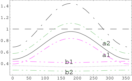
FIG. 1.: CP-averaged branching ratios normalized to $Br(B^{+}\to K^{0}\pi^{+})$ vs. $\gamma$ for $B^{+}\to K^{0}\pi^{+}$ (dashed), $B^{+}\to K^{+}\pi^{0}$ (solid), $B^{0}\to K^{+}\pi^{-}$ (dot-dashed), and $B^{0}\to K^{0}\pi^{0}$ (dotted) for the SM with $m_{s}=100$ MeV. The curves $a_{1},\;b_{1}$ and $a_{2},\;b_{2}$ are for $\Delta g_{1}^{Z}$ equal to $-0.113$ and $0.126$, respectively.

FIG. 2.: Bounds on and (solutions for) $\cos\gamma$ vs. $\delta_{EW}$. The curves a1, a2 (dashed), b (dot-dashed), and c1,c2 (dotted) are the bounds (solutions) on (for) $\cos\gamma$ as functions of $\delta_{EW}$ for the three cases a), b) and c) described in the text, respectively.

REFERENCES

[1] CLEO Collaboration, Y. Kwon et al., CLEO CONF 99-14.
[2] N. Deshpande et al, Phys. Rev. Lett. 82,2240(1999).
[3] M. Neubert and J. Rosner, Phys. Lett. B441, 403(1998).
[4] M. Neubert and J. Rosner, Phys. Rev. Lett. 81, 5074(1998);
M. Neubert, JHEP 9902:014 (1999).
[5] F. Parodi, P. Roudeau and A. Stocchi, e-print hep-ex/9903063.
[6] X.-G. He, Phys. Rev. D53, 6326(1996);
X.-G. He, CP Violation, e-print hep-ph/9710551, in proceedings
of
”CP violation and various frontiers in Tau and other systems”, CCAST, Beijing, 1997.
[7] N. Deshpande, B. Dutta and S. Oh, Phys. Rev. Lett. 77, 4499(1996);
A. Cohen et al., Phys. Rev. Lett. 78, 2300(1997);
Y. Grossman, Y. Nir and M. Worah, Phys. Lett. B407, 307(1997);
M. Ciuchini et. al., Phys. Rev. Lett. 79, 978(1997).
[8] M. Lusignoli, Nucl. Phys. B325, 33(1989);
A. Buras, M. Jamin and M. Lautenbacher, Nucl. Phys. B408, 209(1993);
M. Cuichini et. al., Nucl. Phys. B415, 403(1994).
[9] N. Deshpande and X.-G. He, Phys. Lett. B336, 471(1994).
[10] X.-G. He and B. McKellar, Phys. Rev. D51, 6484(1995);
X-G. He, Phys. Lett. B460, 405(1999).
[11] S.-P. Chia, Phys. Lett. B240, 465(1990);
K. A. Peterson, Phys. Lett. B282, 207(1992);
K. Namuta, Z. Phys. C52, 691(1991);
T. Rizzo, Phys. Lett. B315, 471(1993);
X.-G. He, Phys. Lett. B319, 327(1994);
X.-G. He and B. McKellar, Phys. Lett. 320, 168(1994);
S. Dawson and G. Valencia, Phys. Rev. D49, 2188(1994);
G. Baillie, Z. Phys. C61, 667(1994);
G. Burdman, Phys. Rev. D59, 035001(1999).
[13] A. Ali, G. Kramer and C.-D. Lu, Phys. Rev. D58, 094009(1998).
[14] Particle Data Group, Eur. Phys. J. C3, 1(1998).
[15] For a recent review see, Sinead Ryan, e-print hep-ph/9908386.
[16] X.-G. He, W.-S. Hou and K.-C. Yang, Phys. Rev. Lett. 83,
1100(1999).
[17] R. Fleischer, Phys. Lett. B321, 259(1994);
N. Deshpande, X.-G. He and J. Trampetic, Phys. Lett. B345, 547(1995).
[18] A. Buras and R. Fleischer, e-print hep-ph/9810260.
[19] M. Gerard and J. Weyers, e-print hep-ph/9711469; D. Delepine et al.,
Phys. Lett. B429, 106(1998);
A. Falk et. al., Phys. Rev. D57, 4290(1998); D. Atwood and A. Soni. Phys. Rev.
D58, 036005(1998);
M. Neubert, Phys. Lett. B422, 152(1998);
R. Fleischer, Phys. Lett. B435, 221(1998); Eur. Phys. J. C6,
451(1999);
M. Gronau and J. Rosner, Phys. Rev. D57, 6843(1998);
D58, 113005(1998);
B. Block, M. Gronau and J, Rosner, Phys. Rev. Lett. 78, 3999(1997);
W.-S. Dai et al., e-print hep-ph/9811226 (Phys. Rev. D in press);
X.-G. He, Eur. Phys. J. C9, 443(1999).
[20] R. Fleischer and T. Mannel, Phys. Rev. D57, 2752(1998).
[21] D. London, M. Gronau and J. Rosner. Phys. Rev. Lett. 73,
21(1994).
[22] N. Deshpande and X.-G. He, Phys. Rev. Lett. 74, 26 (E: 4099)(1995).
[23] N. Deshapande, and X.-G. He, Phys. Rev. Lett. 75, 3064(1995); N. Deshpande, X.-G. He and S. Oh, Z. Phys. C74, 359(1997);
M. Gronau et al., Phys. Rev. D52, 6374(1995);
A. Dighe, M. Gronau and J, Rosner, Phys. Rev. D54, 3309(1996);
M. Gronau and J. Rosnar Phys. Rev. Lett. 76, 1200(1996);
R. Fleischer, Int. J. Mod. Phys. A12, 2459(1997).
FIG. 1.:
CP-averaged branching ratios normalized to vs.
for (dashed),
(solid), (dot-dashed), and
(dotted) for the
SM with MeV. The curves and are
for equal to and , respectively.
FIG. 2.:
Bounds on and (solutions for) vs. .
The curves a1, a2 (dashed), b (dot-dashed), and c1,c2 (dotted)
are the
bounds (solutions) on (for)
as functions of for the
three cases a), b) and c) described in the text, respectively.