Path-Integral Formulation of Casimir Effects
in Supersymmetric Quantum Electrodynamics

Abstract

The path-integral method of calculating the Casimir energy between two parallel conducting plates is developed within the framework of supersymmetric quantum electrodynamics at vanishing temperature as well as at finite temperature. The choice of the suitable boundary condition for the photino on the plates is argued and the physically acceptable condition is adopted which eventually breaks the supersymmetry. The photino mass term is introduced in the Lagrangian and the photino mass dependence of the Casimir energy and pressure is fully investigated.

I Introduction

The Casimir effect is an interesting phenomenon in the sense that it provides us with one of the primitive means of extracting the energy out of the vacuum. Since the original work of Casimir[1, 2] a number of works have appeared in extending the result to the case of more general topological and dynamical configurations of the boundary condition and to the circumstances at finite temperature and gravity [3]. In the studies of the Casimir effects it is common to assume the free electromagnetic field in the bounded region. It may be interesting to extend our arguments for fields other than the electromagnetic field. The Casimir effect due to the free fermionic fields has been investigated by several authors and has been found to result in an attractive force under the suitable physical boundary conditions [4, 5].

The supersymmetry is considered to be promising in searching for the unified theory of elementary particles. In this connection it is natural to extend the quantum electrodynamics to incorporate the supersymmetry. It may then be interesting to study the Casimir effect in the supersymmetric quantum electrodynamics in the hope that some evidence of supersymmetry could be observed through the Casimir effect. In the present communication we deal with the Casimir effect by applying the path-integral formulation [6] working in the supersymmetric quantum electrodynamics [7, 8]. In the supersymmetric quantum electrodynamics we have extra particles, photinos (fermions), as superpartners of photons (bosons) and we have to discuss the contributions of photinos as well as photons in the arguments of Casimir effects.

II Path-Integral Formulation

We start with the Lagrangian for the supersymmetric quantum electrodynamics,

$${\mathcal{L}}={\mathcal{L}}_{B}+{\mathcal{L}}_{F},$$ (1)

with

$${\mathcal{L}}_{B}=-\frac{1}{4}F_{\mu\nu}F^{\mu\nu}-\frac{1}{2\alpha}({\partial}^{\mu}A_{\mu})^{2}-i{\bar{\eta}}{\partial}^{\mu}{\partial}_{\mu}{\eta},$$ (2)

and

$${\mathcal{L}}_{F}=-i\lambda{\sigma}^{\mu}{\partial}_{\mu}{\bar{\lambda}},$$ (3)

where $F_{\mu\nu}=\partial_{\mu}A_{\nu}-\partial_{\nu}A_{\mu}$ with $A_{\mu}$ the photon field, the gauge fixing term as well as the Fadeev-Popov term with Fadeev-Popov ghost $\eta$ are included in the Lagrangian ${\mathcal{L}}_{B}$ and $\lambda$ in ${\mathcal{L}}_{F}$ denotes the two-component photino field. We adopt the covariant gauge with gauge parameter $\alpha$. The Fadeev-Popov ghost is usually neglected in quantum electrodynamics since it is irrelevant as far as we consider processes without photon loops and in the normal physical QED processes no photon loop appears. In the Casimir effect, however, we calculate the contribution of the photon loop and so we need to take into account the Fadeev-Popov ghost in order to count correctly the physical degrees of freedom of photons.

We first deal with the Casimir effect at vanishing temperature. Consider the generating functional $Z$ given by

$$Z=\int{[dA_{\mu}][d\eta][d\bar{\eta}][d\lambda]}{[d\bar{\lambda}]}e^{i\int d^{4}x{\mathcal{L}}}$$ (4)

The free energy density $\epsilon$ is related to the generating functional $Z$ through the relation

$$Z=e^{-i\epsilon\Omega},$$ (5)

where $\Omega$ is the space-time volume.

A Photon

The contribution of photons to the generating functional $Z$ is given by

$$Z_{B}=\int{[dA_{\mu}]}{[d\eta]}{[d\bar{\eta}]}e^{i\int d^{4}x{\mathcal{L}}_{B}}.$$ (6)

Performing integration over $A_{\mu}$, $\eta$ and $\bar{\eta}$ we obtain

$$Z_{B}=\left[\textrm{Det}\left(2i\partial^{2}\right)\right]\left[\textrm{Det}(-g_{\mu\nu}\partial^{2}+(1-1/\alpha)\partial_{\mu}\partial_{\nu})\right]^{-1/2},$$ (7)

where the overall factor of the numerical constant is neglected. We note that in momentum space,

$$\det\left[g_{\mu\nu}k^{2}+\left(\frac{1}{\alpha}-1\right)k_{\mu}k_{\nu}\right]=\frac{1}{\alpha}(k_{0}^{2}-k_{1}^{2}-k_{2}^{2}-k_{3}^{2})^{4},$$ (8)

and hence

$$\frac{\ln Z_{B}}{\Omega}=-2\int\frac{d^{4}k}{{(2\pi)}^{4}}ln{(-k^{2})}+\frac{1}{2}\int\frac{d^{4}k}{{(2\pi)}^{4}}(ln\alpha-\frac{i\pi}{2})+\int\frac{d^{4}k}{{(2\pi)}^{4}}ln{(-k^{2})}.$$ (9)

Here in Eq. (9) the first, second and third term come from the $F_{\mu\nu}$ term, the gauge term and the Fadeev-Popov term in the Lagrangian (2) respectively. Since the second term is a constant which is physically irrelevant, we neglect it in the following arguments. We make the Wick rotation in Eq. (9) and find

$$\frac{\ln Z_{B}}{\Omega}=-i\int\frac{d^{4}k}{{(2\pi)}^{4}}\ln k^{2},$$ (10)

for Euclidean momentum $k$. According to the relation (5) the free energy density $\epsilon$ is then easily obtained by performing the integration over the fourth (time) component of the Euclidean four-momentum $k_{\mu}$,

$$\epsilon_{B}=\int{\frac{d^{3}k}{{(2\pi)}^{3}}\sqrt{{\bf k}^{2}}},$$ (11)

where we have neglected the additive constant stemming from the $k_{4}$ integration. Of course the free energy density $\epsilon_{B}$ is a divergent quantity if one considers the infinite space region. In the present argument of the Casimir energy we consider the region bounded by two conducting plates. We place two infinite conducting plates perpendicular to the $z$ direction at $z=0$ and at $z=L$. For photons we introduce the physical boundary condition [1, 2]

$${\bf A}(z=0)={\bf A}(z=L)=0.$$ (12)

According to the condition (12) the $z$-component $k_{z}$ of momentum ${\bf k}$ is discretized such that

$$k_{z}=\frac{\pi n}{L},$$ (13)

with $n$ an integer. Replacing the $k_{z}$ integration by summation on $n$ in Eq. (11) we obtain

$$\epsilon_{B}=\frac{1}{2L}\sum_{n=-\infty}^{\infty}\int\frac{d^{2}k}{{(2\pi)}^{2}}\sqrt{{{\bf k}_{T}}^{2}+{(\pi n/L)}^{2}},$$ (14)

where ${\bf k}_{T}$ refers to the transversal component of ${\bf k}$, i. e., $(k_{x},k_{y})$. The free energy density (14) is a divergent quantity and we regularize it by introducing the regularization factor $e^{-\tau\omega}$ in the integration (14) with $\omega=\sqrt{{{\bf k}_{T}}^{2}+{(\pi n/L)}^{2}}$,

$$\epsilon_{B}=\frac{1}{L}\sum_{n=0}^{\infty}\int\frac{d^{2}k}{{(2\pi)}^{2}}\omega e^{-\tau\omega}.$$ (15)

The integration and summation in Eq. (15) can be easily performed resulting in

$$\epsilon_{B}=\frac{3}{\pi^{2}\tau^{4}}-\frac{{\pi}^{2}}{720L^{4}}.$$ (16)

We distinguish the free energy density for the infinite volume (Eq. (11)) from the one for the bounded region (Eq. (15)) by denoting the former by ${\epsilon_{B}}^{\infty}$. If we use the same regularization as in Eq. (15), we obtain ${\epsilon_{B}}^{\infty}=3/({\pi}^{2}{\tau}^{4})$. The Casimir energy ${\epsilon}_{CB}$ then is given by

$${\epsilon}_{CB}=\epsilon_{B}-{\epsilon_{B}}^{\infty}=-\frac{\pi^{2}}{720L^{4}}.$$ (17)

B Photino

The contribution of photinos to the generating functional $Z$ is given by

$$Z_{F}=\int{[d\lambda]}{[d\bar{\lambda}]}e^{i\int d^{4}x{\mathcal{L}}_{F}}.$$ (18)

After integrating over the photino fields we have $Z_{F}=\textrm{const.}\times\textrm{Det}(i\partial~{}/)$. Going over to the momentum representation and performing the Wick rotation we find

$$\frac{\ln Z_{F}}{\Omega}=i\int{\frac{d^{4}k}{(2\pi)^{4}}\ln k^{2}}.$$ (19)

Then the photino contribution to the free energy density is given by

$$\epsilon_{F}=-\int{\frac{d^{3}k}{{(2\pi)}^{3}}\sqrt{{\bf k}^{2}}}.$$ (20)

For the infinite volume Eq. (20) gives the divergent expression

$${\epsilon_{F}}^{\infty}=-\frac{3}{\pi^{2}\tau^{4}},$$ (21)

with $\tau$ the same regularization parameter as in ${\epsilon_{B}}^{\infty}$.

Consider the bounded region where two parallel plates are placed perpendicular to the $z$ axis at $z=0$ and $z=L$ respectively. The boundary condition for photino fields should be chosen by physical requirements. The physically acceptable requirement may be that there is no fermionic outgoing flux perpendicular to the boundaries. This requirement has been adopted to the MIT bag model long time ago [4, 9]. It is satisfied by the following condition at the boundary plates [5],

$$in~{}/\lambda=\lambda,$$ (22)

where $n_{\mu}=(0,\bf n)$ with $\bf n$ the inward normal to the boundary plates. According to the condition (22) the $z$-component $k_{z}$ of momentum ${\bf k}$ is discretized such that

$$k_{z}=\frac{\pi(2n+1)}{2L},$$ (23)

with $n$ an integer.

It should be noted here that the supersymmetry under consideration is explicitly broken according to the fact that the boundary condition for photinos is different from that for photons. If the supersymmetry is to be respected even in the bounded region, then of course one has to choose a specific (but rather unphysical) boundary condition for photinos in order to maintain the supersymmetry. In our investigation we rather choose the physically acceptable boundary condition for photinos and consider that the supersymmetry is an exact symmetry only for the unbounded space-time. The situation is in some similarity with the finite temperature case where the supersymmetry is broken explicitly according to the different boundary conditions for bosons and fermions respectively.

Replacing the $k_{z}$ integration by summation on $n$ in Eq. (20) we obtain

$$\epsilon_{F}=-\frac{1}{2L}\sum_{n=-\infty}^{\infty}\int\frac{d^{2}k}{{(2\pi)}^{2}}\sqrt{{{\bf k}_{T}}^{2}+{\{\pi(2n+1)/2L\}}^{2}}.$$ (24)

The free energy density (24) is also divergent and we regularize it by using the same regularization factor as in Eq. (15). Performing the summation and integration we obtain

$$\epsilon_{F}=-\frac{3}{\pi^{2}\tau^{4}}-\frac{7}{8}\frac{{\pi}^{2}}{720L^{4}}.$$ (25)

The Casimir energy due to the fermionic effect is given by

$${\epsilon}_{CF}=\epsilon_{F}-{\epsilon_{F}}^{\infty}=-\frac{7}{8}\frac{\pi^{2}}{720L^{4}}.$$ (26)

The total Casimir energy for the supersymmetric quantum electrodynamics is given by summing up the photon and photino contributions and reads

$${\epsilon}_{C}={\epsilon}_{CB}+{\epsilon}_{CF}=-\frac{15}{8}\frac{\pi^{2}}{720L^{4}}.$$ (27)

It is interesting to note here that the divergences appearing in ${\epsilon}_{B}$ and ${\epsilon}_{F}$ cancel out when they are added up and thus

$${\epsilon}_{C}={\epsilon}_{B}+{\epsilon}_{F}.$$ (28)

III Temperature Dependence

We now introduce the temperature. The Matsubara formalism [10] will be employed to introduce temperature effects in the following calculation. We replace the integral in the energy variable $k_{0}$ by the summation where we apply the periodic boundary condition for boson fields and the anti-periodic boundary condition for fermion fields respectively:

$$\int\frac{dk_{0}}{2\pi}f(k_{0})\rightarrow\frac{1}{\beta}\sum_{n=-\infty}^{\infty}f(\omega_{n}),$$ (29)

where $\beta=1/T$ with $T$ the temperature and the energy variable $k_{0}$ in the summation is replaced by $\omega_{n}$ which is given by

$\displaystyle\omega_{n}=\left\{\begin{array}[]{ll}\omega_{n}^{B}\equiv\frac{2n}{\beta}\pi&(\textrm{boson}),\\ \\ \omega_{n}^{F}\equiv\frac{2n+1}{\beta}\pi&(\textrm{fermion}).\end{array}\right.$Repeating the similar calculations as in the previous zero-temperature case we obtain the temperature dependent Casimir energy for photons and photinos respectively:

$$\epsilon_{B}(T)=\frac{1}{2L}\sum_{n=-\infty}^{\infty}[\int\frac{d^{2}k}{{(2\pi)}^{2}}\sqrt{k^{2}}+\frac{2}{\beta}\int\frac{d^{2}k}{{(2\pi)}^{2}}ln(1-e^{-\beta\omega_{B}})],$$ (30)

$$\epsilon_{F}(T)=\frac{1}{2L}\sum_{n=-\infty}^{\infty}[-\int\frac{d^{2}k}{{(2\pi)}^{2}}\sqrt{k^{2}}+\frac{2}{\beta}\int\frac{d^{2}k}{{(2\pi)}^{2}}ln(1+e^{-\beta\omega_{F}})],$$ (31)

where $\omega_{B}$ and $\omega_{F}$ are defined by

$$\omega_{B}=\sqrt{{{\bf k}_{T}}^{2}+{(\pi n/L)}^{2}},\ \ \ \omega_{F}=\sqrt{{{\bf k}_{T}}^{2}+{(\pi(2n+1)/2L)}^{2}}.$$ (32)

Performing the integrations in Eqs. (30) and (31) with the same regularization factors as before we obtain for photons,

$$\epsilon_{B}(T) = \frac{3}{\pi^{2}\tau^{4}}-\frac{{\pi}^{2}}{720L^{4}}$$ (34)

$$-\sum_{n=1}^{\infty}\left(\frac{T^{2}}{n^{2}\pi}\right)^{2}\left\{\frac{n\pi}{2\xi}\coth\left(\frac{n\pi}{2\xi}\right)+\left(\frac{n\pi}{2\xi}\right)^{2}\textrm{cosech}^{2}\left(\frac{n\pi}{2\xi}\right)\right\},$$

and for photinos,

$$\epsilon_{F}(T) = -\frac{3}{\pi^{2}\tau^{4}}-\frac{7}{8}\frac{{\pi}^{2}}{720L^{4}}$$ (36)

$$+\frac{1}{4\pi L^{4}}\sum_{l=1}^{\infty}(-1)^{l}\frac{\xi^{2}}{l^{2}\sinh(l\pi/2\xi)}\left\{\frac{2\xi}{l}+\pi\coth\left(\frac{l\pi}{2\xi}\right)\right\}.$$

where $\xi=L/\beta=LT$ and $\tau$ is the cut-off parameter. The total contribution of photons and photinos in the supersymmetric quantum electrodynamics to the Casimir energy is given by $\epsilon_{C}(T)=\epsilon_{B}(T)+\epsilon_{F}(T)$. We have shown the behaviors of $\epsilon_{C}(T)$ as a function of $T$ for $L$ fixed in Fig. 1. Also shown in Fig. 1 are the individual contribution of photons and photinos to the Casimir energy $\epsilon_{CB}(T)$ and $\epsilon_{CF}(T)$ where the divergent parts in Eqs. (34) and (36) are eliminated as in the case of the vanishing temperature. Note here that for low temperature $\xi\ll 1$

$$\epsilon_{B}(T)=\frac{3}{\pi^{2}\tau^{4}}-\frac{{\pi}^{2}}{720L^{4}}-\frac{{\xi}^{2}}{2L^{4}}\left\{1+\frac{2\xi}{\pi}\right\}e^{-\pi/2\xi},$$ (37)

and for high temperature $\xi\gg 1$

$$\epsilon_{B}(T)=\frac{3}{\pi^{2}\tau^{4}}-\frac{{\pi}^{2}}{720L^{4}}-\frac{7}{8}\frac{{\pi}^{2}}{45}T^{4}$$ (38)

IV Photino Mass Dependence

In our calculations we have kept the photino massless in order to respect the supersymmetry at vanishing temperature. Experimentally, however, the massless photino has not been observed. One of the possibilities of explaining the situation may be that the photino could be extremely massive and is not be observed in the low energy experiments. The photino mass would be generated by some supersymmetry breaking mechanism. We consider this possibility and recalculate the Casimir energy with massive photinos. The calculation is straightforward and the result reads as follows:

$$\epsilon_{F}(T,m)=-\frac{1}{4\pi L}\sum_{n=-\infty}^{\infty}\left\{\frac{{\alpha_{n}}^{2}}{\tau}+\frac{2\alpha_{n}}{\tau^{2}}+\frac{2}{\tau^{3}}\right\}e^{-\tau\alpha_{n}}$$ (39)

$$+\frac{1}{2\pi L}\sum_{n=-\infty}^{\infty}\sum_{l=1}^{\infty}(-1)^{l}\left(\frac{T^{3}}{l^{3}}+\frac{T^{2}}{l^{2}}\alpha_{n}\right)e^{-l{\alpha_{n}}/T},$$ (40)

where $\alpha_{n}=\sqrt{m^{2}+\left(\frac{2n+1}{2L}\pi\right)^{2}}$ with m the photino mass. The behavior of the Casimir energy $\epsilon_{C}$ at vanishing temperature with massive photinos is given in Fig. 2 as a function of the photino mass $m$ together with the individual contributions of photons and photinos respectively.

Finally we calculate the Casimir pressure by differentiating the energy $\epsilon_{C}(T,m)=\epsilon_{B}(T)+\epsilon_{F}(T,m)$ in terms of distance $L$,

$$p(T,m)=-\frac{\partial}{\partial L}[\epsilon_{C}(T,m)L]\Big{|}_{T}.$$ (41)

We have shown the behaviors of $p(T,m)L^{4}$ as a function of $T$ and $m$ in FIG. 3 and 4 respectively. It may be more transparent to show the Casimir energy and the Casimir pressure in the 2 dimensional plot with regards to $T$ and $m$ and those are given in FIG. 5 and 6 respectively.

Judging from the rather strong dependence of the Casimir energy as well as the Casimir pressure on the photino mass as shown in FIG. 5 and 6, it may be rather difficult to detect the evidence of the supersymmetry in the presently accessible experimental situations. We hope that future improvements of the experimental situation will resolve the difficulty.

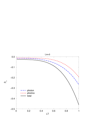
FIG. 1.: The behavior of Casimir energy $\epsilon_{C}L^{4}$ as a function of temperature $LT$. Also shown are $\epsilon_{CB}L^{4}$ and $\epsilon_{CF}L^{4}$ respectively

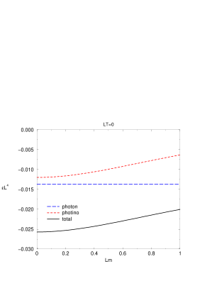
FIG. 2.: The behavior of Casimir energy $\epsilon_{C}(T)L^{4}$ as a function of photino mass $Lm$. Individual contributions $\epsilon_{CB}(T)L^{4}$ and $\epsilon_{CF}(T)L^{4}$ respectively are also shown.

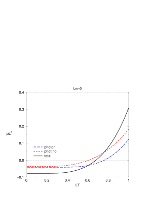
FIG. 3.: The behaviors of Casimir pressure $pL^{4}$ as a function of temperature $LT$.

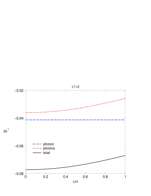
FIG. 4.: The behaviors of Casimir pressure $pL^{4}$ as a function of photino mass $Lm$.

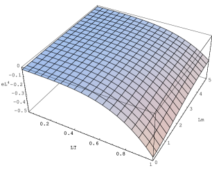
FIG. 5.: The $T$ and $m$ dependence of Casimir energy $\epsilon_{C}(T)L^{4}$.

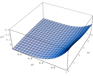
FIG. 6.: The $T$ and $m$ dependence of Casimir pressure $pL^{4}$.

- [1] H. B. G. Casimir, Proc. Kon. Ned. Akad. Wetensch.51 (1948) 793.
- [2] H. B. G. Casimir and D. Polder, Phys. Rev. 73 (1948) 360.
- [3] For a review see, for example, V. M. Mostepanenko and N. N. Trunov, The Casimir Effect and its Applications Clarendon Press, Oxford, 1997
- [4] K. Johnson, Acta Phys. Pol. B6 (1975) 865.
- [5] S. A. Gundersen and F. Ravndal, Ann. Phys. 182 (1988) 90.
- [6] A. K. Ganguly and P. B. Pal, Preprint hep-th/9803009 (1998).
- [7] Y. Igarashi, Phys. Rev. D30 (1984) 1812.
- [8] M. Nakahara, Phys. Lett. 142B (1984) 395.
- [9] A. Chodos, R. L. Jaffe, K. Johnson, C. B. Thorn and V. F. Weisskopf, Phys. Rev. D9 (1974) 3471.
- [10] T. Matsubara, Prog. Theor. Phys. 14(1955) 351.