An efficient renormalization group improved implementation of the MSSM effective potential.

Abstract

In the context of MSSM, a novel improving procedure based on the renormalization group equation is applied to the effective potential in the Higgs sector. We focus on the one-loop radiative corrections computed in Landau gauge by using the mass independent renormalization scheme $\overline{\rm DR}$. Thanks to the decoupling theorem, the well-known multimass scale problem is circumvented by switching to a new effective field theory every time a new particle threshold is encountered. We find that, for any field configuration, there is a convenient renormalization scale $\tilde{Q}^{*}$ at which the loop expansion respects the perturbation series hierarchy and the theory retains the vital property of stability.

I Introduction

The standard model (SM) forms the bedrock of modern high-energy physics, and accurately describes all physical phenomena at energy scales up to $\sim 100$ GeV (electroweak scale). Even in the absence of a grand unification of strong and electroweak (EW) forces at a very high energy scale, it is clear that the SM must be modified to incorporate the effects of gravity at the Planck scale ($M_{P}\simeq 10^{19}$ GeV). In this context, the EW scale is put in by hand and there is no idea about its origin: it is a completely free input parameter. In a more complete theory one would like to understand its origin in terms of more fundamental parameters (e.g., $M_{P}$), but such a theory would need more structure than present in SM.

Moreover, in a general QFT containing an elementary scalar the mass of this scalar would be naturally at the scale of the cutoff of the theory due to the quadratically divergent loop corrections to the scalar self energy (hierarchy problem [1]). If one wants to protect the scalar masses from getting these large loop corrections, one needs to introduce a new symmetry. The only known such symmetry is supersymmetry (SUSY) [2] which relates properties of bosons and fermions. Although there are various ways in which SUSY might be joined with the SM, for simplicity one can pursue a minimal construction and attempt to write down a Lagrangian, which is the most general effective Lagrangian invariant under SUSY transformations up to soft-breaking terms. This then results in the Lagrangian of the Minimal Supersymmetric Standard Model (MSSM) [3], where each SM particle is accompanied by a supersymmetric partner. Supersymmetry also requires two Higgs doublets, as opposed to the single Higgs doublet of the SM.

One of the most remarkable features of the MSSM is that it offers a plausible senario for $SU(2)_{L}\times U(1)_{Y}$ symmetry breaking. However, in this senario one has still to enforce phenomenologically a bounded from below potential and the absense of directions in field space that may induce a spontaneous breaking of electric and/or color charge symmetries [4] (a fact that clearly violates experimental observations).

From the theoretical point of view, in the SM electric and color charge are certainly conserved in an automatical way, since the only fundamental scalar field is the Higgs boson, a colorless electroweak doublet. The Higgs potential has a continuum of degenerate minima, but these are all physically equivalent and one can always define the unbroken $U(1)_{Y}$ generator to be the electric charge. On the contrary, in SUSY extensions of SM things become more complicated. Since the Higgs sector contains at least two Higgs doublets $H_{1},H_{2}$, one has to check that the minimum of the Higgs potential still occurs for values of $H_{1},H_{2}$ which are appropriately aligned in order to preserve the electric charge. Another perplexity arises from the fact that the supersymmetric theory (MSSM) has a large number of additional charged and color scalar fields, namely all the sleptons $(\tilde{\ell})$ and squarks $(\tilde{q})$. Consequently, conservation of color and electric charge symmetries requires that the minimum of the whole potential $V(H_{1},H_{2},\tilde{\ell},\tilde{q})$ still occurs at a point in the field space where $\langle\tilde{q}\rangle,\langle\tilde{\ell}\rangle=0$ (realistic or true minimum).

Yet, the true effective potential in which the vacuum structure is encoded, is a poorly known object beyond the tree-level approximation. One reason for this is the dependence of its loop corrections upon the very many different mass scales present in MSSM, so that a renormalization group (RG) analysis becomes rather tricky. In general, when one deals with a system possessing a large mass scale $Q_{M}$, compared with the scale $Q_{\mu}$ at which one discusses physics, large logarithms such as $\ln(Q_{M}/Q_{\mu})$ always appear which affect the convergence of the perturbative realization of the potential (loop expansion). In this situation, one considers resumming the perturbation series by using the renormalization group equation. Nonetheless, in many relistic applications one often has to deal with an additional mass scale $Q_{m}$ with the hierarchy $Q_{\mu}\ll Q_{m}\ll Q_{M}$. In MSSM, for instance, one can regard $Q_{\mu},Q_{m},Q_{M}$ as the weak, supersymmetry-breaking and unification scales respectively. When we study such a system, we face the problem of multimass scales [5, 6, 7, 8, 9]: There appear several types of logarithms $\ln(Q_{M}/Q_{\mu})$ and $\ln(Q_{m}/Q_{\mu})$, while we are able to sum up just a single logarithm by means of the RG equation.

But is it really necessary to take into account these obscure loop corrections? Naively, one would argue that they cannot change much of the qualitative pattern of the tree level minima. On these grounds, let us recall that classical potential in MSSM receive contribution from three sources: D-terms, F-terms and soft-breaking terms. The first of these provides the quartic terms $V_{D}=\lambda\varphi^{4}$ with $\lambda>0$. Now along special directions in field space, known as D-flat directions, $V_{D}\sim 0$ can occur. If there is a minimum in such a direction, then the change in the shape of the potential near the vicinity of that minimum, due to one-loop corrections, could create perturbatively a supplementary local minimum lower than that already present at tree level. In other words, even if the one-loop corrected effective potential is expected to differ, point-to-point, only perturbatively from its tree level value, it is still possible that its shape be locally modified in such a way that new local minima (or at least stationary points) appear.

Clearly, a carefull RG improvement program is then essential in order to deal with the physical problems already mentioned. Trying to illuminate this missing point, in the present work a generalized improving procedure based on [10] is applied to the MSSM effective potential. The main idea of the method is to make use of the decoupling theorem [11]. By this theorem, it is made sufficient to treat essentially a single log factor at any renormalization scale, since all the heavy particles (heavier than that scale) decouple and all the light particles (lighter than that scale) yield more or less the same log factors.

The rest of the paper will be organized as follows. After setting our notation and conventions, the state of the art concerning the EW symmetry breaking in MSSM is briefly reviewed in Sec. II. In the next two sections, we describe the physical difficulties we have faced in trying to extrapolate the well known low energy picture of MSSM to higher energies and how they have been overcome. A detailed presentation of our numerical implementation is given in Secs. V–VI, while Sec. VII explains the reasoning behind our renormalization scale choise. The final section is devoted to conclusions and further comments. Detailed formulae for the various field dependent MSSM mass eigenstates in a neutral Higgs background are presented in Appendix A and some special cases of them in Appendix B. Finally, last two Appendices include technical details essential to our numerical procedure, as well as a description of the numerical algorithms used for our purposes.

II Setting up the frame

A The Lagrangian

We are dealing with the MSSM i.e., the simplest supersymmetrized version of the SM. The requirements of minimal particle content and matter parity conservation immediately dictate the expression of the $SU(3)_{C}\times SU(2)_{L}\times U(1)_{Y}$ invariant superpotential

$${\cal W}={\bf Y_{e}}{\hat{L}}^{j}{\hat{E}}^{c}{\hat{H}}_{1}^{i}\epsilon_{ij}+{\bf Y_{d}}{\hat{Q}}^{ja}{\hat{D}}_{a}^{c}{\hat{H}}_{1}^{i}\epsilon_{ij}+{\bf Y_{u}}{\hat{Q}}^{ja}{\hat{U}}_{a}^{c}{\hat{H}}_{2}^{i}\epsilon_{ij}+\mu{\hat{H}}_{1}^{i}{\hat{H}}_{2}^{j}\epsilon_{ij}$$ (1)

where the chiral matter superfields transform as follows
$\bullet$ Quark Superfields : ${\hat{Q}}={\hat{u}\atopwithdelims( )\hat{d}}=\kern-3.20007pt\raisebox{0.58122pt}{$\stackrel{{\scriptstyle\mbox{.}}}{{\mbox{.}}}\kern 2.70004pt$}({\bf 3},{\bf 2},1/6)$, ${\hat{U}}^{c}=\kern-3.20007pt\raisebox{0.58122pt}{$\stackrel{{\scriptstyle\mbox{.}}}{{\mbox{.}}}\kern 2.70004pt$}(\overline{{\bf 3}},{\bf 1},-2/3)$, ${\hat{D}}^{c}=\kern-3.20007pt\raisebox{0.58122pt}{$\stackrel{{\scriptstyle\mbox{.}}}{{\mbox{.}}}\kern 2.70004pt$}(\overline{{\bf 3}},{\bf 1},1/3)$
$\bullet$ Lepton Superfields : ${\hat{L}}={\hat{\nu}\atopwithdelims( )\hat{\ell}}=\kern-3.20007pt\raisebox{0.58122pt}{$\stackrel{{\scriptstyle\mbox{.}}}{{\mbox{.}}}\kern 2.70004pt$}({\bf 1},{\bf 2},-1/2)$, ${\hat{E}}^{c}=\kern-3.20007pt\raisebox{0.58122pt}{$\stackrel{{\scriptstyle\mbox{.}}}{{\mbox{.}}}\kern 2.70004pt$}({\bf 1},{\bf 1},1)$
$\bullet$ Higgs Superfields : ${\hat{H}}_{1}={\hat{{\cal H}}_{1}\atopwithdelims( )\hat{h}_{1}}=\kern-3.20007pt\raisebox{0.58122pt}{$\stackrel{{\scriptstyle\mbox{.}}}{{\mbox{.}}}\kern 2.70004pt$}({\bf 1},{\bf 2},-1/2)$, ${\hat{H}}_{2}={\hat{h}_{2}\atopwithdelims( )\hat{{\cal H}}_{2}}=\kern-3.20007pt\raisebox{0.58122pt}{$\stackrel{{\scriptstyle\mbox{.}}}{{\mbox{.}}}\kern 2.70004pt$}({\bf 1},{\bf 2},1/2)$
under the aforementioned gauge group. Note that the free parameter $\mu$ and the $3\times 3$ Yukawa matrices ${\bf Y_{u}}$, ${\bf Y_{d}}$, ${\bf Y_{e}}$ are generally complex. These ingredients are enough to specify a globaly supersymmetric gauge invariant Lagrangian : ${\cal L}_{SUSY}$.

The fact that SUSY is not observed at low energies requires the introduction of extra supersymmetry breaking interactions. This breaking, however, should be such that no quadratic divergences appear and the technical “solution” to the hierarchy problem is not spoiled. Such terms are generally termed “soft” [12] and are interpreted as remnants of the spontaneous breaking of local SUSY in the underlying fundamental theory (Supergravity (SUGRA) [13] or Superstrings [14]). They include :

• Mass terms for all scalar fields.

• Gaugino mass terms.

• Biliner scalar interactions.

• Trilinear scalar interactions.

Consequently, the most general SUSY breaking interaction Lagrangian with real mass terms, resulting from spontaneously broken SUGRA in the flat limit $(M_{P}{\rightarrow}{\infty})$ is

$${\cal L}_{SOFT} = -{1\over 2}M_{1}(\tilde{B}\tilde{B})-{1\over 2}M_{2}(\tilde{W^{\Gamma}}\tilde{W^{\Gamma}})-{1\over 2}M_{3}(\tilde{G^{R}}\tilde{G^{R}})$$ (5)

$$-m_{H_{1}}^{2}|H_{1}|^{2}-m_{H_{2}}^{2}|H_{2}|^{2}-m^{2}_{\tilde{Q}}|\tilde{Q}|^{2}-m^{2}_{\tilde{D}^{c}}|\tilde{D}^{c}|^{2}-m^{2}_{\tilde{U}^{c}}|\tilde{U}^{c}|^{2}$$

$$-m^{2}_{\tilde{L}}|\tilde{L}|^{2}-m^{2}_{\tilde{E}^{c}}|\tilde{E}^{c}|^{2}-({\bf h_{e}}\tilde{L}^{j}\tilde{E}^{c}H_{1}^{i}\epsilon_{ij}+{\bf h_{d}}\tilde{Q}^{ja}\tilde{D}_{a}^{c}H_{1}^{i}\epsilon_{ij}$$

$$+{\bf h_{u}}\tilde{Q}^{ja}\tilde{U}_{a}^{c}H_{2}^{i}\epsilon_{ij}+\mbox{H.c.})-(B\mu H_{1}^{i}H_{2}^{j}\epsilon_{ij}+\mbox{H.c.})$$

We denote with $H_{1}$, $H_{2}$ the ordinary Higgs boson doublets and with $\tilde{Q}$, $\tilde{D}^{c}$, $\tilde{U}^{c}$, $\tilde{L}$, $\tilde{E}^{c}$ the squark and slepton scalar fields. On the other hand, the gauginos $\tilde{B}$, $\tilde{W}$, $\tilde{G}$, are considered as two component Weyl spinors and ${\bf h}\equiv{\bf Y}{\bf A}$, where A is a $3\times 3$ matrix containing the “soft” trilinear scalar couplings. All extra soft parameters except masses are generally complex. This completes the picture for the low-energy effective theory.

Altogether one would then need more than 100 real parameters to discribe soft SUSY breaking in full generality. Clearly, some simplifying assumptions are necessary if we want to achieve something close to a complete study of parameter space. The following set of assumptions is adopted:

• We shall work in the approximation of vanishing intergenerational mixing i.e.,
  ${\bf Y_{e}}=\mbox{diag}(Y_{e}^{1},Y_{e}^{2},Y_{e}^{3}),\quad{\bf Y_{u}}=\mbox{diag}(Y_{u}^{1},Y_{u}^{2},Y_{u}^{3}),\quad{\bf Y_{d}}=\mbox{diag}(Y_{d}^{1},Y_{d}^{2},Y_{d}^{3})$
  where all non-zero entries are real and positive.

• $\mu$, $B$ and all trilinear soft couplings are real.
  (The phases of these parameters give large one-loop contributions to CP violating quantities, so practically they are quite constrained [15].)

• In our analysis we shall also keep Yukawas and trilinear soft couplings from light families, since their contributions to the one-loop effective potential (our main objective) are not always negligible for an arbitrary field configuration.

A dramatic simplification of the structure of the SUSY-breaking interactions is provided either by grand unification assumptions or by superstrings. The simplest possible choise arising from coupling the MSSM to minimal $N=1$ SUGRA is the following set of assumptions:

• Common gaugino mass : $m_{1/2}$

• Common scalar mass : $m_{0}$

• Common trilinear scalar coupling : $A_{0}$

at a very large scale $M_{X}$. More complicated alternatives also exist. However for the time being, for the sake of setting our notation, we shall focus on this “universal” senario.

This reduces the number of free parameters describing SUSY breaking to just four : The gaugino mass $m_{1/2}$, the scalar mass $m_{0}$, the trilinear and bilinear soft breaking parameters $A_{0}$ and $B$. We do assume unification of the gauge couplings at scale $M_{X}\simeq 2\times 10^{16}$ GeV. At this point, no specific relation is assumed for the Yukawa couplings at grand unification scale (GUT).

In order to discuss the physical implications of this Lagrangian at low-energy, we need to renormalize the relevant parameters at experimentally accesible energies by computing them from a set of coupled renormalization group equations (RGE) [17]. (A detailed discussion of this procedure will be given in the following sections). This leads us to radiative gauge symmetry breaking which we now consider.

B RG improvement and electroweak breaking

The effective potential in general admits a loop expansion [18] as :

$$\hat{V}_{eff}(\lambda_{\alpha},\phi;Q)=\hat{V}_{eff}(\lambda_{\alpha},0;Q)+\sum_{n=1}^{\infty}{1\over n!}\phi^{n}\Gamma^{(n)}(p_{i}=0)$$ (6)

where $\hat{V}_{eff}(\lambda_{\alpha},0;Q)$ is a non-trivial function that receives contributions from all orders in perturbation theory, $\lambda_{\alpha}$ are the couplings of the theory, $Q$ is a mass parameter upon which it explicitly depends and $\Gamma^{(n)}$ are the connected proper vertices at zero external momenta. Using a particular regularization scheme, one can get rid of the infinities by absorbing them into the renormalization of the basic parameters of the theory ($\lambda_{\alpha},\phi$). The resulting parameters become then $Q$ dependent and their evolution is determined by the beta functions $\beta_{\alpha}$ (couplings) and the anomalous dimensions $\gamma$ (fields). When a similar renormalization program is applied to $\hat{V}_{eff}$, order by order in perturbation series, the resulting potential function ${\cal V}_{eff}$ can be cast in a formally $Q$-dependent loopwise expansion

$${\cal V}_{eff}(\lambda_{\alpha}(Q),\phi(Q);Q)=\sum^{\infty}_{n=0}V^{(n)}=V^{(0)}+V^{(1)}+\ldots$$ (7)

Since $Q$ is an unphysical quantity, the potential in Eq. (7) should not depend on the choise of it. This property can be achieved, if a change in the scale $Q$ can be compensated by appropriate changes in the couplings and field rescalings. Mathematically it can be formulated by a RG equation satisfied by the effective potential

$$\left(Q{d\over dQ}+\beta_{\alpha}{\partial\over\partial\lambda_{\alpha}}-\gamma\phi{\partial\over\partial\phi}\right)V_{eff}=0$$ (8)

which admits the solution

$$V_{eff} = V_{eff}(\lambda_{\alpha}(Q),\phi(Q);Q)$$ (9)

$$= \Omega^{\prime}+{\cal V}_{eff}\qquad\qquad\qquad(\Omega^{\prime}:\mbox{ $\phi$ independent shift})$$ (10)

$$= \Omega^{\prime}+V^{(0)}+V^{(1)}+\ldots$$ (11)

The point is that unless $\Omega^{\prime}$ is specifically chosen, then $V_{eff}$ fails to satisfy the RG equation of the usual form [7, 19, 20, 21]. The obvious choise for $\Omega^{\prime}$ is of course $\Omega^{\prime}=-\sum_{n=0}^{\infty}V^{(n)}(\phi=0)$. From a practical point of view, adding a field independent piece to $V_{eff}$ is perfectly harmless in problems where only field derivatives of $V_{eff}$ are of interest and a constant value is assigned to $Q$.

An appealing feature of the MSSM is that it can lead to the breaking of electroweak symmetry radiatively [17, 22]. The correct $SU(2)_{L}\times U(1)_{Y}$ breaking down to $U(1)_{em}$ is achieved by restricting the vacuum expectation values (vevs) on the neutral Higgs manifold

$$\langle H^{i}_{1}\rangle={\cal H}_{1}\delta^{i}_{1},~{}~{}~{}~{}\langle H^{i}_{2}\rangle={\cal H}_{2}\delta^{i}_{2},~{}~{}~{}~{}\langle\tilde{q}\rangle=0,~{}~{}~{}~{}\langle\tilde{\ell}\rangle=0$$ (12)

Here $\delta^{i}_{j}$, ($i,j=1,2$) is the well known Kronecker symbol, ${\cal H}_{1}$, ${\cal H}_{2}$ are taken real by gauge freedom and the last two equalities have to be satisfied by all the scalar quarks and leptons of the model. The low energy classical scalar potential along this direction is then

$$V^{(0)}=m_{1}^{2}|{\cal H}_{1}|^{2}+m_{2}^{2}|{\cal H}_{2}|^{2}+2m_{3}^{2}({\cal H}_{1}{\cal H}_{2})+{g^{2}+g_{2}^{2}\over 8}(|{\cal H}_{1}|^{2}-|{\cal H}_{2}|^{2})^{2}$$ (13)

where $m_{1}^{2}=m_{H_{1}}^{2}+\mu^{2}$, $m_{2}^{2}=m_{H_{2}}^{2}+\mu^{2}$, $m_{3}^{2}=\mu B$ and $g$, $g_{2}$ are the $U(1)$ and $SU(2)$ gauge couplings.

On the other hand, the one-loop effective Higgs potential of the model, in Landau gauge using the $\overline{\rm DR}$ renormalization scheme [23], is

$$V^{(1)} = {k\over 4}\;Str\!\left\{{\cal M}^{4}\left(\ln{{\cal M}^{2}\over Q^{2}}-{3\over 2}\right)\right\}$$ (14)

$$= k\sum_{p\atop(M_{p}^{2}\not=0)}V^{(1)}_{p}$$ (15)

$$V^{(1)}_{p} = {(-1)^{2S_{p}}\over 4}(2S_{p}+1)\,C_{p}\,{\cal N}_{p}\,M_{p}^{4}(\phi)\left(\ln{|M_{p}^{2}(\phi)|\over Q^{2}}-{3\over 2}\right)$$ (16)

where $k=(16\pi^{2})^{-1}$ and ${\cal M}^{2}$ is the field dependent tree level squared mass matrix of the model. We denote by $M_{p}$ the mass eigenvalue of the ${\rm p}^{\rm th}$ particle and $S_{p}$, $C_{p}$ are its associated spin, color degrees of freedom. ${\cal N}_{p}$ is the number of its helicity states ($p$ runs over all particles), $\phi$ are the shifted scalar fields and $Q$ is the renormalization scale. Finally, at one-loop order we have

$$\Omega^{\prime}=-V^{(1)}(\lambda_{\alpha}(Q),\phi(Q)=0;Q)$$ (17)

so

$$V_{1-loop}=\Omega^{\prime}+V^{(0)}+V^{(1)}$$ (18)

The parameters of the potential are taken as running ones, that is they vary with scale according to the two loop RGEs with one loop thresholds in all running parameters [24, 25].

Before carrying on, we would like to comment on a subtle point in $V^{(1)}$ definition. We know that at any acceptable minimum all the eigenvalues of ${\cal M}^{2}$ must be positive, otherwise an imaginary part appears in $V^{(1)}$. This problem arises because of the non-convexity of the tree level potential $V^{(0)}$ [6, 26], when the gauge symmetry is spontaneously broken. In our case, particularly in the Higgs sector, if we compute the tree level field dependent mass eigenvalues for the values $(v_{1}^{0},v_{2}^{0})$ which minimize $V^{(0)}$ at low-energies, some of them would certainly vanish (Goldstone modes). On the other hand, when we try to find the true minimum $(v_{1},v_{2})$ of $V_{1-loop}$, negative mass eigenvalues in the Higgs sector may now appear. However, since these negative eigenvalues are of ${\cal O}(\hbar)$, we can practically take the absolute value of $M_{p}^{2}$ inside the logarithm [28].

Given the low energy scale of EW breaking we must use the renormalization group to evolve the parameters of the potential to a convenient scale such as $M_{Z}$ (physical Z-boson mass), where the experimental values of the gauge couplings are usually referred. In contrast to the tree level potential, $V_{1-loop}$ is relatively stable with respect to $Q$ around the electroweak scale [20, 28, 29, 30]. Therefore, the exact scale at which to minimize is no longer critical as long as it is in the electroweak range.

A glance at the superpotential (1) shows that $H_{2}$ couples to the $t$ (s)quarks, while $H_{1}$ only couples to $b$ (s)quarks and $\tau$ (s)leptons by means of the Yukawa couplings. These Yukawa couplings enter the RGEs for square scalar masses with positive sign. So their effect is always to decrease the Higgs masses as one evolves the RG equations downward from GUT scale to $M_{Z}$. Combined with the experimental fact that top quark is heavy, this can cause the RG-evolved $m_{H_{2}}^{2}$ to run negative near the EW scale, helping to destabilize the point ${\cal H}_{1}={\cal H}_{2}=0$ and so triggering the breaking of gauge symmetry. If we define

$$\overline{m}_{i}^{2} = m_{i}^{2}+\Sigma_{i}~{}~{}~{}~{}~{}(i=1,2)~{}~{}~{}~{}~{}~{}\mbox{where}$$ (19)

$$\Sigma_{i} = {1\over 2{\cal H}_{i}}\>{\partial\over\partial{\cal H}_{i}}V^{(1)}$$ (20)

$$= {k\over 4}\sum_{p\atop(M_{p}^{2}\not=0)}(-1)^{2S_{p}}(2S_{p}+1)\,C_{p}\,{\cal N}_{p}{1\over{\cal H}_{i}}\>{\partial M_{p}^{2}\over\partial{\cal H}_{i}}\>f(M_{p}^{2};Q)$$ (21)

with

$$f(x,Q) = x\left(\ln{|x|\over Q^{2}}-1\right)$$ (22)

then the minimization of the potential yields the following two conditions among its parameters (all parameters are $Q$ dependent)

$$\sin 2\beta = -\frac{2B\mu}{\overline{m}_{1}^{2}+\overline{m}_{2}^{2}}$$ (24)

$$\frac{1}{2}m_{Z}^{2}(M_{Z}) = \frac{\overline{m}_{1}^{2}-\overline{m}_{2}^{2}\tan^{2}\beta}{\tan^{2}\beta-1}$$ (25)

where $m_{Z}^{2}(M_{Z})$ is the running mass of the Z boson and $\tan\beta=v_{2}/v_{1}$. Note that in the above relations $\Sigma_{i}$ include contributions from all particles (see Appendix A), $Q$ takes a constant value $(M_{Z})$ and derivatives are taken with respect to running fields ${\cal H}_{1}(Q),\ {\cal H}_{2}(Q)$, so there is no contribution from vacuum energy $(\partial\Omega^{\prime}/\partial{\cal H}_{i}(Q)=0)$. Moreover, since all the scalar fields ($\phi$) are multiplicative renormalizable, we conclude that if $\phi(Q_{0})=0$, for some $Q_{0}$, then $\phi(Q)=0$ for every $Q$. This is what actually happens for all scalar fields except Higgses (see Eq. (12)).

Of course, we do not merely want $SU(2)_{L}\times U(1)_{Y}$ to be broken; we also want the Z boson to have the experimentally measured mass ($M_{Z}$). Furthermore, in view of the strong dependence of some weak-scale quantities on $\tan\beta$, it is often more convenient to treat $M_{Z}$ as an independent input parameter. Since $m_{Z}^{2}={1\over 2}(g^{2}+g_{2}^{2})(v_{1}^{2}+v_{2}^{2})$, fixing $m_{Z}$ (equivalently $M_{Z}$) and $\tan\beta$ determines both vevs $v_{1},v_{2}$.

For all that, destabilizing the origin by a negative $({\rm mass})^{2}$ parameter is not enough to ensure the viability of the MSSM one loop scalar potential. We must also make sure that the potential is bounded from below for arbitrarily large values of the scalar fields, so that Eq. (18) will really have a minimum.

III Attempts to deal with high energies

Extending this well known low-energy picture to high-energies (large field values), one is confronted with peculiar effective potential configurations. The simplest generalization is allowing Higgs fields, in Eqs. (13)–(15), to take arbitrary values keeping at the same time the renormalization scale fixed at $M_{Z}$. However, this assumption leads to an unbounded from below (UFB) potential. This realization is clearly physically undesirable. Before explaining the reason behind such a failure, let us see what causes this fake instability.

Let ${\cal H}_{1}=x_{1}$, ${\cal H}_{2}=x_{2}$ and calculate all the field dependent mass eigenvalues in polar coordinates

$$x_{1}=r\cos\theta,\qquad\qquad x_{2}=r\sin\theta$$ (26)

With no harm of generality, as shortly will be seen, we’ll only take contributions from $3^{\rm rd}$ family. We intent to write $V_{1-loop}$ for $r\gg 1$. For our approximation to hold, coefficients that multiply powers of $r$ should not be arbitrarily small. So, for each $r$, our approximation is valid only for those values of $\theta$ that respect the above constraint. Choosing $\theta=\pi/2$ and using the formulae in Appendix B the potential becomes after some algebra

$$V_{1-loop}=V^{(0)}+V^{(1)}+\mbox{ (field independent piece)}$$ (28)

where

$$V^{(0)}(r\gg 1)=m_{2}^{2}r^{2}+\frac{g^{2}+g_{2}^{2}}{8}r^{4}\simeq\frac{g^{2}+g_{2}^{2}}{8}r^{4}$$ (29)

$$64\pi^{2}V^{(1)}(r\gg 1)=r^{4}\left({\cal A}\,s(r)+\sum_{i=1}^{11}d_{i}U_{i}^{2}\ln\frac{|U_{i}|}{Y_{t}^{2}}\right)$$ (30)

$${\cal A}=\frac{2g^{4}}{3}+\frac{(g^{2}-3g_{2}^{2})^{2}}{24}-3Y_{t}^{2}(g^{2}+g_{2}^{2})+\sum_{i=1}^{9}d_{i}U_{i}^{2}$$ (31)

In the above, $s(r)=\ln(Y_{t}^{2}r^{2}/\tilde{Q}^{2})$, $\tilde{Q}=Qe^{3/4}$ and $d_{i},U_{i}$ are given in Appendix B. The crucial term for determining the behavior of the function presented above is the logarithmic coefficient $({\cal A})$. This number due to large top Yukawa coupling is negative, so the whole function is UFB. (Note that should we have taken contributions from light families, nothing would have changed since top quark Yukawa coupling still dominates).

Apparently, the main tool of our discussion is the loop expansion. So ultimately one has to justify the convergence of loop expansion at high energies, ensuring in this way that only the first terms in the series should be kept. Eventually, one has to study the logarithmic structure of the effective potential. It has been shown in [7, 19] that the L-loop effective potential contains logarithmic factors, only up to L-th power, whose magnitude control the convergence of the loop expansion. These factors have the general form

$$s=\lambda\ln\frac{M^{2}(\phi_{c})}{Q^{2}}$$ (32)

where $\lambda$ is some coupling of the theory, $M$ is a field dependent mass eigenvalue in the presence of the background fileds $\phi_{c}$ and $Q$ is the renormalization scale. In our case (MSSM), large field values generate large (field dependent) mass eigenvalues and obviously large log-factors ($Q$ is fixed at $M_{Z}$). So higher order corrections (2-loops etc.) become significant and should also be taken into account. These corrections should raise the potential because the theory should be stable and can not have an UFB potential. In conclusion, the one-loop approximation to the effective potential renormalized at $M_{Z}$ for large field values is not reliable and a different scale choise to control large logs is needed.

An alternative way of thinking about RG improvement is to view it as a reorganization of the perturbation series, in which the first term is the sum of all the leading logarithms, the second term represents the next-to-leading logarithms, and so on [7, 8, 19, 21]. The leading logarithms are terms of the form $u^{(n)}\ln(M_{1}(\phi)/Q)\ln(M_{2}(\phi)/Q)\cdots\ln(M_{n}(\phi)/Q)$ and represent the most “dangerous” logarithmic terms at each order in perturbation theory. If we could fully sum the multiscale leading and next-to-leading logs, we should have an approximation that is useful dispite the existence of widely differing scales. However, when there is more than one mass scales present it is less clear how to proceed; no choise of $Q$ will destroy all the logarithms simoultaneously.

This point of view is adopted in the improvement prescription presented in [7]. Let us briefly describe it. Imagine a theory (like MSSM) having many coupling constants and mass scales. The problem in such multiscale cases is which log-factor we should choose to sum up the leading, next-to-leading etc. logs. The best choise would be to take a particle whose coupling constant is the largest. Calling that particle by label $k=0$ we have

$$s_{0}=\lambda_{0}\ln\frac{M_{0}^{2}(\phi_{c})}{Q^{2}}$$ (34)

$$s_{k}=\lambda_{k}\ln\frac{M_{k}^{2}(\phi_{c})}{Q^{2}}={\lambda_{k}\over\lambda_{0}}\,s_{0}+u_{k}\qquad\mbox{where}\qquad u_{k}=\lambda_{k}\ln\frac{M_{k}^{2}(\phi_{c})}{M_{0}^{2}(\phi_{c})}$$ (35)

If it happens all the masses $M_{k}^{2}(\phi_{c})$ be of the same order independently of the background scalar fields $\phi_{c}$, then $u_{k}$ variables remain always of order ${\cal O}(\lambda_{k})\lesssim{\cal O}(\lambda_{0})$. So all the log factors essentially can be treated as $s_{0}$ or $(\lambda_{k}/\lambda_{0})s_{0}$, since the differences $u_{k}$ are of order higher than the first $s_{0}$ term. In this case, the field dependent scale $Q^{2}=M_{0}^{2}(\phi_{c})\Leftrightarrow s_{0}=0$ correctly sums all logs in the leading-log series expansion, improving thus succesfully the effective potential.

We have numerically applied the prescription described above to MSSM and suprisingly found that with this scale prescription the effective potential values near $x_{1}=\pm x_{2}$ direction (H-diag) are quite unexpected. H-diag direction, for large field values, develops saddle points (near 200 TeV! as shown in Fig. 1a) which lead to an unphysical (UFB) potential. Unfortunately, near H-diag direction field dependent mass eigenvalues far away from origin are not all of the same order (see Appendix B). So some of the $u_{k}$ are large and one has to keep any higher powers of them in the leading-log series expansion. This in turn implies that higher loop corrections are significant and can not be neglected. In other words, the absense of a unique scale choise (even field dependent), that eliminates large logs to all orders, makes the improvement prescription of Ref. [7] for MSSM unreliable.

This deceptive deadlock of course steams from our careless treatment of different mass scales by a single scale parameter $Q$. Hiding all the heavy particle loop contributions in the redefinition of the low energy theory parameters, we can still solve the same RG equation for the effective potential by using different effective field theories. This will be the subject of the next section.

IV An alternative senario : V-thresholds

Recently, the authors of Ref. [10] have proposed a nice method to realize the attractive conjecture just mentioned. Specifically, one should use the decoupling theorem to handle with the problem of many scales in the effective potential, using as decoupling scale for the mass eigenvalue $M^{2}(\phi)$ the scale

$$\tilde{Q}^{2}=|M^{2}(\phi)|$$ (36)

(recall that $\tilde{Q}=Qe^{3/4}$). In other words, we use the following expansion as our impoved potenial

$$V^{(1)}=k\sum_{i}V_{i}^{(1)}\theta_{i}$$ (38)

$$\theta_{i}\equiv\theta\Big{(}\tilde{Q}^{2}-|M_{i}^{2}(\phi)|\Big{)}$$ (39)

$$V_{i}^{(1)}=\frac{(-1)^{2S_{i}}}{4}(2S_{i}+1)\,C_{i}\,{\cal N}_{i}\,M_{i}^{4}(\phi)\ln\frac{|M_{i}^{2}(\phi)|}{\tilde{Q}^{2}}$$ (40)

Despite the appearance of Heaviside functions the effective potential is a continuous function (a discontinous potential is physically meaningless). A discontinuity is likely to appear only at a decoupling point (threshold). Let’s examine what is happening when $\tilde{Q}^{2}$ approaches the $\ell^{\rm th}$ threshold. We have

• Just above the threshold :

  
  

  $\displaystyle[V^{(1)}]_{\epsilon_{+}}=k\sum_{i=1}^{\ell-1}\,[V_{i}^{(1)}\theta_{i}]_{\epsilon_{+}}+k\,[V_{\ell}^{(1)}\theta_{\ell}]_{\epsilon_{+}}$

• Just below the threshold :

  
  

  $\displaystyle[V^{(1)}]_{\epsilon_{-}}=k\sum_{i=1}^{\ell-1}\,[V_{i}^{(1)}\theta_{i}]_{\epsilon_{-}}$

• At the threshold :

  
  

  $\displaystyle[V^{(1)}]_{\epsilon=0}=k\sum_{i=1}^{\ell-1}\,[V_{i}^{(1)}\theta_{i}]_{\epsilon=0}+k\,[V_{\ell}^{(1)}\theta_{\ell}]_{\epsilon=0}$

But $V_{\ell}^{(1)}\propto M_{\ell}^{4}(\phi)\ln(|M_{\ell}^{2}(\phi)|/\tilde{Q}^{2})$ and as $\tilde{Q}^{2}\rightarrow|M_{\ell}^{2}(\phi)|$ (i.e., $\epsilon\rightarrow 0$), then $[V_{\ell}^{(1)}\theta_{\ell}]_{\epsilon=0}=0$ and $[V_{\ell}^{(1)}\theta_{\ell}]_{\epsilon_{+}}=0$ so, the potential function is continuous as it should be.

On the other hand, defining

$$\Sigma_{i}^{*}={1\over 2{\cal H}_{i}}\sum_{k}\frac{\partial V_{k}^{(1)}}{\partial{\cal H}_{i}}\theta_{k}\equiv\sum_{k}\Psi^{(k)}_{i}\theta_{k}$$ (41)

the corrections $\Sigma_{i}$ of Eq. (2.12) become in this new approach

$$\Sigma_{i}=\Sigma_{i}^{*}-{1\over 2{\cal H}_{i}}\sum_{k}V_{k}^{(1)}\,\delta\Big{(}\tilde{Q}^{2}-|M_{k}^{2}(\phi)|\Big{)}\,{\partial|M_{k}^{2}|\over\partial{\cal H}_{i}}$$ (42)

The last term is obviously zero, so the stationary conditions have the well known form of Eqs. (2.14a)–(2.14b) replacing $\Sigma_{i}$ with the new $\Sigma_{i}^{*}$ .

Let us recall that we are working in the one-loop approximation, which is scale independent up to 2-loop corrections. These corrections, however, may be very large due to the presence of potentially large logarithms in $V^{(n>1)}$. Thus, one has to be careful in choosing a value of Q which gives the finest approximation to $V_{1-loop}$. We’ll come back to this critical issue during the numerical method’s description, but for completeness we stress here that in the above stated framework the potential is indeed bounded from below as Fig. 1b shows.

V Numerical procedure for radiative ew breaking

In this section, following the analysis of [24] we shall present the procedure we use to restrict the SUSY parameter space to those regions, where the requirement of radiative breaking of electroweak sector can be correctly implemented.

The generic problem, we have to tackle here, could be formulated as a set of coupled first-order ordinary differential equations (ODEs) for the dependent variables (running parameters) $y_{i}$, $i=1,2,\ldots,n$ having the form

$$y^{\prime}_{i}(t)=f_{i}(y_{1},y_{2},\ldots,y_{n})$$ (43)

where the functions $f_{i}$ on the right-hand side are known and $t\equiv 2\ln(M_{X}/Q)$ is the independent variable (scale). However, a problem involving ODEs is not completely specified by its equations. Initial conditions (values of the running parameters $y_{i}$) must also be supplied at some starting point $t_{a}$ which in our case is: $t_{a}=0$ i.e., $Q=M_{X}$. The underlying idea of any numerical routine, that solves an initial value problem, is to propagate the solution $y_{i}$ over an interval $[t_{a},t_{b}]$ with $t_{b}\not=t_{a}$, using a step-by-step calculation, which approximates values of the solution at discrete specified points in that interval. As far as the MSSM case is concerned, we have used special routines from NAG fortran library (which is available to us) and particularly an Adams variable-order variale-step algorithm, which provides a choise of automatic error control and an option of a sophisticated root-finding technique [31].

The initial conditions at $M_{X}$ scale will be choosen as simple as possible postponing for elsewhere the study of more complicated alternatives. Thus, at the unification point taken to be ${\cal O}(10^{16})$ GeV, we shall take

$$m_{\tilde{Q}}(M_{X})=m_{\tilde{D}^{c}}(M_{X})=m_{\tilde{U}^{c}}(M_{X})=m_{0}$$ (45)

$$m_{\tilde{L}}(M_{X})=m_{\tilde{E}^{c}}(M_{X})=m_{0}$$ (46)

$$m_{H_{1}}(M_{X})=m_{H_{2}}(M_{X})=m_{0}$$ (47)

and

$$M_{1}(M_{X})=M_{2}(M_{X})=M_{3}(M_{X})=m_{1/2}$$ (48)

In addition we take equal cubic couplings at $M_{X}$, i.e.,

$$A_{e}(M_{X})=A_{d}(M_{X})=A_{u}(M_{X})=A_{0}$$ (49)

Obviously, all our “universal” boundary conditions are family blind.

Contact has to be made between the low-energy and high energy parameters of the theory [32]. This will be achieved by integrating the RGEs from a superheavy scale, taken to be in the neighborhood of $10^{16}$ GeV, down to a scale $Q_{0}\gtrsim M_{Z}$. In order to make a run starting from $M_{X}$ we must have the values of all parameters at this scale, something difficult to achieve. The problem is that the values of many parameters are known experimentally at low scales. Also 1-loop stationary contitions are applied at such low energies. However, the values of other parameters, such as soft breaking terms, are most easily understood at higher energies, where theoretical simplification (e.g., universality) may be invoked. Thus, there is no scale at which both theoretical simplicity and experimental confirmation coexist.

Moreover, MSSM is characterized by two kinds of parameters, constrained and free. The former are constrained by experiment (gauge couplings, quark masses etc.) or by relations among themselves (stationary conditions at $M_{Z}$). The latter, given the present experimental data, can not be constrained by these two critiria and must be viewed as input parameters. These are $A_{0}$, $B_{0}$, $\mu_{0}$ (values at $M_{X}$), $m_{1/2}$, $m_{0}$, $\tan\beta$ (ratio of vevs at $M_{Z}$) and $M_{t}$ (physical mass for the top quark). In the present framework, $B_{0}$ and $\mu_{0}$ will be determined using the numerical integration routines in conjuction with the minimization of the one loop effective potential at $M_{Z}$ (i.e., Eqs. (2.14a)–(2.14b)). Namely, stationary conditions at $M_{Z}$ will give $B(M_{Z})$, $\mu(M_{Z})$ and then we run back up to $M_{X}$ in order to determine $B_{0}$ and $\mu_{0}$. Note that the sign of $\mu$ is not determined from (2.14a)–(2.14b), thus we must make a choise for it. So ultimately the free parameters of the theory are taken to be

$$A_{0},~{}m_{0},~{}m_{1/2},~{}\tan\beta,~{}M_{t},~{}{\rm sign}(\mu)$$ (50)

On the other hand, the exact values of the constrained parameters at $M_{X}$ are affected by the choise of values for the free parameters at that scale, since the evolution of all parameters are coupled.

We begin our numerical procedure at the EW scale which we take to be $M_{Z}$. This is an obvious choise, since many experimental quantities are now available at that scale. At $Q=M_{Z}$ we take as input the well measured values of the Z mass $M_{Z}=91.1867\pm 0.0020$ GeV, the electromagnetic coupling constant $\alpha_{em}^{-1}(M_{Z})|_{\overline{MS}}=127.88\pm 0.09$ [33] and the weak mixing angle $(\sin^{2}\theta_{W})|_{\overline{MS}}=0.2316-0.88\times 10^{-7}(M_{t}^{2}-160^{2}){\rm GeV}^{-2}$ [34]. In addition to the values of the gauge couplings at $Q=M_{Z}$ one also needs the Yukawa couplings of quarks and leptons there. In order to determine $(Y_{\tau},Y_{b})\equiv(Y_{e}^{3},Y_{b}^{3})$ at $M_{Z}$, we run the gauge couplings $\alpha$ and $\alpha_{3}$ from their experimental values at $M_{Z}$ down to the $b$- and $\tau$-mass scales using three-loop QCD and two-loop QED RGEs [35]. The relevant procedure is described with all details in [24]. Finally, the top Yukawa coupling ($Y_{t}$) is obtained from the running $t$-quark mass, which for our input value $M_{t}=174$ GeV is $m_{t}(M_{Z})\simeq M_{t}/\left(1+{5\alpha_{3}\over 3\pi}\right)\simeq 162$ GeV.

The evolution of all couplings from $M_{Z}$ running upwards to higher energies determines the unification scale $M_{X}$ and the value of the unification coupling $\alpha_{X}$ (in $\overline{\rm DR}$) by

$$\hat{\alpha}_{1}(M_{X})=\hat{\alpha}_{2}(M_{X})=\alpha_{X}$$ (51)

Running down from $M_{X}$ to $M_{Z}$ the trial input value for $\alpha_{3}$ has now changed. The entire procedure is repeated several times. After one third of iterations is completed, we introduce finite part contributions to our low energy inputs such as QCD corrections to the top quark, gluino mass and weak mixing angle $\sin^{2}\theta_{W}|_{\overline{DR}}$. Also the gauge couplings values $\hat{\alpha}_{1}$, $\hat{\alpha}_{2}$ (in $\overline{\rm DR}$) are now determined in terms of Fermi Constant $G_{F}=1.16639\times 10^{-5}\,{\rm GeV}^{-2}$, the Z boson mass and the electromagnetic coupling $\hat{\alpha}_{EM}^{-1}=137.036$ [33]. For details on these matters see Ref. [36]. The running $t$, $b$, $\tau$ quark masses at $M_{Z}$ are now defined through the

$$m_{f}(M_{Z})=M_{f}+\Pi_{f}(Q=M_{Z})$$ (52)

where $M_{f}$ is the physical mass and $\Pi_{f}$ is the self energy corrections of the fermion. This new procedure is now iterated until convergence is reached. When convergence is established, the following actions are taken place at renormalization point $M_{Z}$ :

• Light Yukawa couplings are being computed dividing the fermion masses [33] by the appropriate Higgs vev. These couplings are considered as fixed with respect to $Q$. On the other hand, the light trilinear scalar couplings do run.

• The whole set of the MSSM running parameters values (gauge - Yukawa couplings, soft masses - couplings and Higgs vevs) is stored for later use (improvement of effective potential around EW scale).

• MSSM running parameters are evolved from their current values at $M_{X}$ to a lower scale $Q_{high}$. $Q_{high}$ is taken bigger than the largest field dependent mass eigenvalue appearing in $V^{(1)}$, when the background scalar fields are restricted in a hypercube of side $S_{\infty}$. This point will be clarified later, but for the moment we simply state that $Q_{high}\simeq 5S_{\infty}$ is a more or less satisfactory approximation for our purposes.

Finally, our results should be reconciled with

• Basic experimental constraints on supersymmetric masses as well as Higgs bosons masses as shown in Table I [33].

• Radiative electroweak breaking (existence of real non-zero vevs).

• Positivity of eigenvalues of the mass matrix. Negative eigenvalues mean that expanding around realistic minimum tachyonic states appear making the true minimum of the theory unstable.

VI Threshold parametrization for $\beta$-functions

In the minimall low energy SUGRA model being considered, the super-particle spectrum is no longer degenerate. This should lead to various course corrections, each one occuring at the super-particle mass thresholds. So the renormalization group $\beta$-functions must be cast in a new form, which makes the implementation of the threshold effects evident. Since the $\overline{\rm DR}$ RGEs are mass independent, each super-particle mass determines a boundary between two effective theories. Above a particular mass threshold the associated particle is present, whereas in the effective theory below the threshold the particle is absent.

The simplest way to incorporate this is to treat the thresholds as steps in the particle content of the renormalization group $\beta$-functions [24, 30]. Let’s briefly outline the procedure. Assume that $b$ is the beta function of a running parameter in the $\overline{\rm DR}$ scheme. The corresponding RGE should be integrated from a superlarge scale $M_{X}$ down to any desirable value of $Q$. As we come down from $M_{X}$, as long as we are at scales larger than the heaviest particle in the spectrum, we include in $b$ contributions from all particles in the MSSM. When we cross the heaviest particle threshold, we switch in a new effective field theory with the heaviest particle integrated out and of course a new $b$. Coming further down in energy, we encounter the next particle threshold at which point we switch again to a new effective field theory with the two heaviest particles integrated out and a new $b$. That procedure goes on until all particles are exchausted.

Crossing a particle’s threshold means that the renormalization scale has become smaller than its physical mass. Hence, we need a condition to determine the exact point of decoupling (i.e., decoupling scale). For field configurations in the low energy regime ($\lesssim 300$ GeV) this is simply

$$\tilde{Q}^{2}=m^{2}(Q),\qquad\tilde{Q}=Qe^{3/4}$$ (53)

where $m^{2}(Q)$ is the running soft parameter corresponding to the particle. Consequently, the step functions in RGEs will have the form

$$\theta_{m}=\theta\Bigl{(}\tilde{Q}^{2}-m^{2}(Q)\Bigr{)}$$ (54)

Alternatively, for all other field configurations we shall use a different condition to fix the decoupling point of a particle. Our condition now is

$$\tilde{Q}^{2}=|M^{2}(\phi;Q)|$$ (55)

where $M^{2}$ is the field dependent mass eigenvalue for that particle. Analogously, the step functions in RGEs will become

$$\theta_{M}=\theta\Bigl{(}\tilde{Q}^{2}-|M^{2}(\phi;Q)|\Bigr{)}$$ (56)

This procedure is generally more accurate than the approximation stated in Eq. (53), but in the case of true minimum it introduces non-trivial field dependence, through mass eigenvalues, in $\Sigma_{1}^{*}$, $\Sigma_{2}^{*}$ and the simple stationary conditions (2.14) become extremely involved. (For a presentation of the relevant $m^{2}$, $M^{2}$ see Appendix C.)

VII Choosing the scale

Our starting point is that the full effective potential is independent of the renormalization point $Q$ and thus satisfies the RGE

$${dV_{eff}\over dQ}=0$$ (57)

One can imediately write down the general solution to (7.1) introducing the “running” distance $t$ from the initial values as :

$$V_{eff}=V_{eff}(\lambda_{\alpha}(t),\phi(t);Q(t))=\Omega^{\prime}+V^{(0)}+V^{(1)}+{\cal O}(\hbar^{2})$$ (59)

$$Q(t)=M_{X}e^{-t/2},~{}~{}~{}~{}~{}~{}~{}~{}~{}~{}\Omega^{\prime}=-V^{(1)}(\phi=0)$$ (60)

where $\lambda_{a}(t)$ are all dimensionless and dimensionfull couplings of the MSSM and $\phi(t)=\zeta(t)\phi_{c}$ are the running fields with $\zeta(t)=\exp\{-\int_{0}^{t}dt^{\prime}\gamma(t^{\prime})\}$, $\gamma(t)$ being the anomalous dimension of the $\phi$ field. The key to the usefulness of the RG is that we can choose a value of $t$ such that the perturbation series converges more rapidly than the series for $t=0$. Moreover, there is nothing to stop us choosing a different value of $t$ for each value of $\phi$.

In order to validate the use of 1-loop effective potential one must ensure that not only the couplings be perturbative, but that the loop expansion be convergent as well. In problems with only one mass scale RG improvement is straightforward. But for the cases of interest here there are several mass scales, so one must think up an improvement prescription. Moreover, the lack of analytic formulae describing the scale dependence of the quantities involved, as well as the absence of any profound physical reasoning for choosing the appropriate scale make this task quite obscure.

Earlier attempts [20, 28, 29, 30, 37] can not offer a substantial aid, since their object was an improvement in the low energy region. For example, Ref. [28] argues that there is a scale $\hat{Q}$ where one-loop stationary configuration coincides with the tree level one. Thus by definition

$$\left.{\partial V^{(1)}\over\partial{\cal H}_{i}}\right|_{\hat{Q}}=0$$ (61)

The above definition is non-trivial to implement, so one should approximate $\hat{Q}$ with an average of dominant field dependent masses. For $|{\cal H}_{i}|<10^{5}$ GeV this is a legitimate approximation, but when extending for $|{\cal H}_{i}|\gtrsim 10^{5}$ GeV the potential develops an unphysical UFB escape along H-diag direction which forces us to search for something else.

Recently, another point of view have been introduced in Ref. [10]. Namely, one should compute at a scale $Q_{R}$ where both

$$\left.V^{(1)}\right|_{Q_{R}}\simeq 0$$ (63)

$$\left.{dV_{1-loop}\over dQ}\right|_{Q_{R}}\simeq 0$$ (64)

are satisfied. Clearly, for this $Q_{R}$ the radiative corrections to tree level are small and our approximation to the full potential has the least Q-dependence. We have tried to implement the above prescription to MSSM, but the result is rather discouraging. The field dependent spectrum of MSSM always consists of masses at the order of $M_{Z}$ (coming from the neutralino sector). So application of (63) will lead to a critical scale around $M_{Z}$, which as we saw gives a problematic potential. On the other hand, (64) seems much more reasonable in the sense that the potential will be more scale independent. However, in this case our numerical routines can not provide us with a scale for every field point $({\cal H}_{1},{\cal H}_{2})$. Due to the step functions in RGEs the integration routine has to take too many intrinsic steps to preserve stability and accuracy of the solution. This in turn affects the performance and the numerical root finding facility when invoked for the equation (64).

To overcome this ambiguity in MSSM, we shall make a physically motivated choise of scale which reproduces a well behaved bounded from below effective potential one expects in a stable theory. Before carrying on, for clarity reasons, let us sketch briefly the behaviour of $V^{(1)}$ near H-diag direction. Without harm of generality, we choose to examine the dominant contribution of top-stop sector. The corresponding partial sums of $V^{(1)}$ are

$$\mbox{Top :}\quad P_{t}=-2\,{\cal C}M_{t}^{4}\ln{|M_{t}^{2}|\over\tilde{Q}^{2}}\,\theta_{t},~{}~{}~{}~{}~{}~{}\mbox{Stops :}\quad P_{T_{i}}={\cal C}M_{T_{i}}^{4}\ln{|M_{T_{i}}^{2}|\over\tilde{Q}^{2}}\,\theta_{T_{i}}$$ (65)

where ${\cal C}$ is some constant factor and $\theta_{t},~{}\theta_{T_{i}}$ ($i=1,2$) are the associated step functions. For non-zero partial sums we must take $\tilde{Q}>|M_{t}|,|M_{T_{i}}|$, i.e., $\ln{|M^{2}|\over\tilde{Q}^{2}}<0$ for all $M$ involved ($P_{t}>0$ and $P_{T_{i}}<0$). As we approach H-diag bottom points, the field dependent top-stop eigenvalues conspire to produce an extremely large negative contribution to $V^{(1)}$ which is responsible for the UFB escape.

However, such a picture can not be reconciled with a perturbation series hierarchy, neither with the notion of stability every acceptable physical theory should have. Consequently, $\tilde{Q}$ should be taken such as top-stop and similar “heavy” pairs are decoupled, see Figs. 2a-b, making loop expansion meaningfull ($|V^{(0)}|\gtrsim|V^{(1)}|$). One such rather conservative choise is $\tilde{Q^{*}}=10^{-3}\sqrt{{\cal H}_{1}^{2}+{\cal H}_{2}^{2}}$ for large ${\cal H}_{i}$ (${\cal H}_{i}\gtrsim 10^{8}$ GeV). Note that for this choise as ${\cal H}_{1},{\cal H}_{2}$ approach $M_{Z}$, $Q^{*}$ will become lower than $M_{Z}$ making the RGE evolution ambiguous. The situation can be improved by defining

$$\tilde{Q^{*}}=10^{\omega(x)}\sqrt{{\cal H}_{1}^{2}+{\cal H}_{2}^{2}}$$ (66)

where $x={1\over 2}\log{{\cal H}_{1}^{2}+{\cal H}_{2}^{2}\over L^{2}}$ is the order of magnitude of a generalized “radious” in the field space and $L=1~{}{\rm GeV}$ makes the log argument dimensionless.

In the context of the approach we have followed, it seems rather non trivial to rigorously define $\omega(x)$. So one has to look for a qualitative fixing. Specifically, as $x$ decreases, field dependent masses decrease too, therefore $\tilde{Q}^{*}$ should decrease, otherwise the non-zero partial sums in $V^{(1)}$ could produce points deeper than the EW minimum. Using the cubic spline interpolation method [42, 45] we can give an ansatz for $\omega(x)$, see Figs. 3a-b, compatible with continuity and the following constraints : (a) $Q^{*}\gtrsim M_{Z}$, (b) $|V^{(0)}|\gtrsim|V^{(1)}|$, (c) $\omega(9)\simeq-3$ in order to recover the previously stated conservative choise for $\tilde{Q}^{*}$, (d) as ${\cal H}_{i}\rightarrow M_{Z}$, $Q^{*}\rightarrow M_{Z}$ i.e.,

$$\omega(x)=\cases{\omega_{c}-x&if $\quad x\leq x_{c}$\cr A_{11}(A_{12}+x)(A_{13}+x)(A_{14}+x)&if $\quad x_{c}<x\leq 4$\cr A_{21}(A_{22}+x)(A_{23}+x)(A_{24}+x)&if $\quad 4<x\leq 5$\cr A_{31}(A_{32}+x)(A_{33}+A_{34}x+x^{2})&if $\quad 5<x\leq 6$\cr A_{41}(A_{42}+x)(A_{43}+A_{44}x+x^{2})&if $\quad 6<x\leq 8$\cr A_{51}(A_{52}+x)(A_{53}+A_{54}x+x^{2})&if $\quad 8<x$\cr}$$ (67)

where by definition $x_{c}=\log(300\sqrt{2})$, $\omega_{c}=\log({M_{Z}\over L}e^{3/4})$ and the coefficients $A$ are shown below

$$A=\left(\begin{array}[]{cccc}-0.691121&-4.17735&-4.&-2.39498\\ 0.389965&-6.31201&-4.2182&-4.\\ -0.176436&-4.46928&37.1171&-11.5691\\ 0.115471&-10.7737&27.1562&-10.2237\\ -0.0417777&-6.09931&183.38&-26.1999\\ \end{array}\right)$$ (68)

To complete this picture one also needs some “boundary scale” $Q_{high}$, which shall provide the starting values of the running parameters for the evolution at $Q^{*}$. One convenient choise is an intermediate scale higher than the largest field dependent mass eigenvalue at the current field point. Specifically, at some field point ${\cal H}=\max({\cal H}_{1},{\cal H}_{2})$ we approximately have $\max_{k}\{\sqrt{|M_{k}^{2}({\cal H}_{1},{\cal H}_{2})|}\}\simeq{\cal H}$. Let $S_{\infty}$ denotes the upper bound order of magnitude of the allowed values for the fields. Then valid choises for $Q_{high}$ are : $\tilde{Q}_{high}\gtrsim S_{\infty}\Rightarrow Q_{high}\gtrsim S_{\infty}e^{3/4}\simeq 2.12\,S_{\infty}$. This is reasonable since the SM is supposed to be a low-energy effective theory coming from a more fundamental theory.

Specifying the scale $Q_{high}$ is not enough. We also need to know the values of the running parameters and fields there. Since $Q_{high}$ is above all thresholds, the required values sould not depend on the background fields and the reasonable choise at an arbitrary field point is

$$\lambda_{\alpha}(Q_{high};{\cal H}_{1}(Q_{high}),{\cal H}_{2}(Q_{high}))\equiv\lambda_{\alpha}(Q_{high};v_{1},v_{2})$$ (69)

where $v_{1}$, $v_{2}$ are the vevs of the EW minimum. In other words, to find the LHS of Eq. (69) we simply integrate the RGE from $M_{X}$ to this new $Q_{high}$ using as initial conditions at $M_{X}$ the outcome of the iteration procedure described in Sec. V. Evolving this set of values $\{{\cal H}_{1}(Q_{high}),{\cal H}_{2}(Q_{high}),\lambda_{\alpha}(Q_{high};v_{1},v_{2})\}$ to $Q^{*}$, using field dependent thresholds, the effective potential at the current field point can be constructed.

VIII Conclusions

In the framework of MSSM, the fact that the top quark is heavy suggests an interesting possibility for explaining the spontaneous symmetry breaking at the EW scale, i.e., the radiative breaking senario. The key method to analyze such a senario is based on the RG equation. In describing the radiative symmetry breaking, the most primitive approach is to use the tree level Higgs potential with the RG running masses and couplings inserted. There exists, however, a serious technical problem in finding symmetry breaking solutions. Namely, the results often depend badly on the choise of the renormalization point $Q$ at which the RG running is terminated, a fact that clearly reduces their reliability.

As emphasized by the authors of Refs. [20, 28, 29, 30, 37], addition of the one-loop corrections $V^{(1)}$ to the classical potential ameliorates the scale dependence at least for low energies. However, we have ascertained with surprise, that a careless treatment of these corrections for high energies formally jeopardizes the stability of the theory. Along a special direction (H-diag), where the magnitude of tree level potential $V^{(0)}$ is small, these corrections when carelessly treated predominate and produce an undesirable UFB escape. The reason behind such a failure must be sought in the inadequacy of a mass independent renormalization scheme $(\overline{\rm DR})$ to treat the very many mass scales of MSSM as one. The problem is that the decoupling of the various particles is not automatically included in the formalism and has to be incorporated.

So to achieve our purpose we have tried to implement the decoupling theorem in a manner proposed by the authors of Ref. [10]. A simple way to incorporate it in the MSSM case is to treat the various particle thresholds as steps in the $\beta$-functions, as well as in the one loop corrections of the scalar potential. Each time we cross a threshold the $\beta$-function changes indicating that we have switched to a new effective field theory with the heaviest particle integrated out. At the same time, the associated particle’s contribution to $V^{(1)}$ is dropped realizing in this way the process of decoupling. We stress here the role played by the renormalization scale choice, as given in Sec. VII. It should be wisely chosen in order to eliminate heavy particles whose participation induces a fake instability, while at the same time improve the convergence of the loop expansion (i.e., $|V^{(1)}|\lesssim|V^{(0)}|$).

Employing the framework just stated and using the “merlin” minimization program [38] (for details see Appendix D) we have scanned the dangerous H-diag direction in its entirety in order to reveal unexpected local minima different than the true. This procedure has been repeated for a representative set of initial conditions at $M_{X}$, but the outcome was always the same: a bounded from below potential with a $SU(3)_{C}\times U(1)_{Y}$ symmetric minimum at EW scale.

Clearly, since the described method allows to undertake faraway excursions in the field space it can be utilized in less investigated situations. For instance, in the past various authors have focused on conditions (involving soft trilinear scalar couplings), which are needed to ensure that a particular SUSY model avoids an electric and/or color charge breaking ground state. However, to our opinion a careful numerical analysis of the impact the one-loop corrections $V^{(1)}$ would have on these matters, is still required. Due to their inherent complexity and for the sake of presenting analytic expressions, one usually resorts to getting round contrivances in order to efficiently deal with the problem. On the other hand, from our numerical point of view, we can directly attack the problem of radiative corrections at the cost of loosing track of analytic elegance. These issues will be the subject of a forthcoming publication [39].

A Field dependent spectrum of MSSM

We give here all the field dependent mass eigenstates of the MSSM in the presence of a neutral Higgs background and the necessary expressions $(\Psi_{i})$ to compute $\Sigma_{i}^{*}$ of Eq. (41). Similar formulae can also be found in Ref. [40]. To simplify somehow the expressions we switch to the notation ${\cal H}_{1}=x_{1},~{}{\cal H}_{2}=x_{2}$. The function $f(x)$, frequently used below, has already been defined in Sec. II, as well as the rest of the notation.

  $\bullet$ Gauge Bosons

$(W^{\pm},Z)$

$$M^{2}(W^{\pm})={g_{2}^{2}\over 2}(x_{1}^{2}+x_{2}^{2})\qquad M^{2}(Z)={g^{2}+g_{2}^{2}\over 2}(x_{1}^{2}+x_{2}^{2})$$ (A.1)

and

$$\Psi_{1}(W^{\pm})=\Psi_{2}(W^{\pm}) = {3g_{2}^{2}\over 32\pi^{2}}f\Bigl{(}M^{2}(W^{\pm})\Bigr{)}\qquad$$ (A.2)

$$\Psi_{1}(Z)=\Psi_{2}(Z) = {3(g^{2}+g_{2}^{2})\over 64\pi^{2}}f\Bigl{(}M^{2}(Z)\Bigr{)}\qquad$$ (A.3)

  $\bullet$ Leptons

$(\ell:e,\mu,\tau)$

$$M^{2}({\ell})=(Y_{\ell}\,x_{1})^{2}$$ (A.4)

and

$$\Psi_{1}(\ell)=-{Y_{\ell}^{2}\over 8\pi^{2}}f\Bigl{(}M^{2}(\ell)\Bigr{)}\qquad\qquad\Psi_{2}(\ell)=0$$ (A.5)

  $\bullet$ Up-Quarks

$({\cal Q}:u,c,t)$

$$M^{2}({\cal Q})=(Y_{{\cal Q}}\,x_{2})^{2}$$ (A.6)

and

$$\Psi_{1}({\cal Q})=0\qquad\qquad\Psi_{2}({\cal Q})=-{3Y^{2}_{{\cal Q}}\over 8\pi^{2}}f\Bigl{(}M^{2}({\cal Q})\Bigr{)}$$ (A.7)

  $\bullet$ Down-Quarks

$(q:d,s,b)$

$$M^{2}(q)=(Y_{q}\,x_{1})^{2}$$ (A.8)

and

$$\Psi_{1}(q)=-{3Y^{2}_{q}\over 8\pi^{2}}f\Bigl{(}M^{2}(q)\Bigr{)}\qquad\qquad\Psi_{2}(q)=0$$ (A.9)

  $\bullet$ Gluinos

$$M^{2}(\tilde{G})=M^{2}_{3}\qquad\Longrightarrow\qquad\Psi_{1}(\tilde{G})=\Psi_{2}(\tilde{G})=0$$ (A.10)

However, with a “vacuum energy” subtraction ($\Omega^{\prime})$ their contribution is canceled from $V_{1-loop}$.

  $\bullet$ Charginos

$(C_{1},C_{2})$
Field dependent mass matrix:

$${\cal M}^{T}_{C}{\cal M}_{C}=\left(\begin{array}[]{cc}M_{2}^{2}+g_{2}^{2}x_{1}^{2}&-g_{2}(\mu x_{1}+M_{2}x_{2})\\ -g_{2}(\mu x_{1}+M_{2}x_{2})&\mu^{2}+g_{2}^{2}x_{2}^{2}\end{array}\right)$$ (A.11)

Its eigenvalues $M^{2}(C_{k})=\lambda_{k}(x_{1},x_{2}),~{}k=1,2$ are roots of the characteristic equation :

$$\lambda^{2}-b_{1}\lambda+b_{0}=0$$ (A.12)

with $b_{1}=\mu^{2}+M_{2}^{2}+g_{2}^{2}(x_{1}^{2}+x_{2}^{2})\quad\mbox{and}\quad b_{0}=(\mu M_{2}-g_{2}^{2}x_{1}x_{2})^{2}$. Obviously $b_{0},b_{1}>0$ so there are two real and positive roots. Easily :

$${1\over x_{i}}{\partial\lambda_{k}\over\partial x_{i}}={1\over 2}\left[{1\over x_{i}}{\partial b_{1}\over\partial x_{i}}+{{b_{1}\over x_{i}}{\partial b_{1}\over\partial x_{i}}-{2\over x_{i}}{\partial b_{0}\over\partial x_{i}}\over{\rm sign}(\lambda_{k}-\lambda_{\ell\not=k}){\cal D}_{C}}\right]\quad(i,\ell=1,2)$$ (A.13)

where

$${\cal D}_{C}=\sqrt{b_{1}^{2}-4b_{0}}=\sqrt{(\mu+M_{2})^{2}+g_{2}^{2}(x_{1}-x_{2})^{2}}\;\sqrt{(\mu-M_{2})^{2}+g_{2}^{2}(x_{1}+x_{2})^{2}}$$ (A.14)

Finally

$$\Psi_{i}(C_{k})=-{1\over 16\pi^{2}}\,{1\over x_{i}}{\partial\lambda_{k}\over\partial x_{i}}\,f(\lambda_{k})$$ (A.15)

  $\bullet$ Neutralinos

$(N_{1},N_{2},N_{3},N_{4})$
Field dependent mass matrix:

$${\cal M}_{N}=\left(\begin{array}[]{cccc}M_{1}&0&gx_{1}/\sqrt{2}&-gx_{2}/\sqrt{2}\\ 0&M_{2}&-g_{2}x_{1}/\sqrt{2}&g_{2}x_{2}/\sqrt{2}\\ gx_{1}/\sqrt{2}&-g_{2}x_{1}/\sqrt{2}&0&-\mu\\ -gx_{2}/\sqrt{2}&g_{2}x_{2}/\sqrt{2}&-\mu&0\\ \end{array}\right)$$ (A.16)

Mass eigenvalues $M(N_{k})=\lambda_{k}(x_{1},x_{2}),~{}k=1,2,3,4$ are roots of the characteristic equation :

$$\lambda^{4}+A_{1}\lambda^{3}+A_{2}\lambda^{2}+A_{3}\lambda+A_{4}=0$$ (A.17)

It is straightforward to show that

$$A_{1} = -M_{1}-M_{2}$$ (A.18)

$$A_{2} = -\mu^{2}+M_{1}M_{2}-(g^{2}+g_{2}^{2})(x_{1}^{2}+x_{2}^{2})/2$$ (A.19)

$$A_{3} = \mu^{2}(M_{1}+M_{2})-\mu(g^{2}+g_{2}^{2})x_{1}x_{2}+(M_{1}g_{2}^{2}+M_{2}g^{2})(x_{1}^{2}+x_{2}^{2})/2$$ (A.20)

$$A_{4} = -\mu^{2}M_{1}M_{2}+\mu(M_{1}g_{2}^{2}+M_{2}g^{2})x_{1}x_{2}$$ (A.21)

Differentiation of Eq. (A.17) gives

$${1\over x_{i}}{\partial\lambda_{k}\over\partial x_{i}} = -{\vartheta_{ik}\over\vartheta^{\prime}_{k}}\qquad(i=1,2)$$ (A.22)

$$\vartheta_{ik} = {1\over x_{i}}{\partial A_{1}\over\partial x_{i}}\lambda_{k}^{3}+{1\over x_{i}}{\partial A_{2}\over\partial x_{i}}\lambda_{k}^{2}+{1\over x_{i}}{\partial A_{3}\over\partial x_{i}}\lambda_{k}+{1\over x_{i}}{\partial A_{4}\over\partial x_{i}}$$ (A.23)

$$\vartheta^{\prime}_{k} = 4\lambda_{k}^{3}+3A_{1}\lambda_{k}^{2}+2A_{2}\lambda_{k}+A_{3}$$ (A.24)

Finally

$$\Psi_{i}(N_{k})=-{1\over 32\pi^{2}}\,{1\over x_{i}}{\partial\lambda_{k}^{2}\over\partial x_{i}}\,f(\lambda_{k}^{2})$$ (A.25)

  $\bullet$ Sneutrinos

$(\tilde{\nu}_{\ell})\qquad(\ell:e,\mu,\tau)$

$$M^{2}(\tilde{\nu}_{\ell})=m^{2}_{\tilde{L}}+{1\over 4}\,(g^{2}+g_{2}^{2})(x_{1}^{2}-x_{2}^{2})$$ (A.26)

and

$$\Psi_{1}(\tilde{\nu}_{\ell})=-\Psi_{2}(\tilde{\nu}_{\ell})={g^{2}+g_{2}^{2}\over 64\pi^{2}}\,f\Bigl{(}M^{2}(\tilde{\nu}_{\ell})\Bigr{)}$$ (A.27)

  $\bullet$ Other scalars

$(\varphi_{1},\varphi_{2})\quad$ All other scalars can be grouped into independent subsets. These are: Sleptons $(\tilde{\ell}_{1},\tilde{\ell}_{2})$, Up-Squarks $(\tilde{\cal Q}_{1},\tilde{\cal Q}_{2})$, Down-Squarks $(\tilde{q}_{1},\tilde{q}_{2})$ and Higgses $(H^{+},H^{-}),~{}(h,H),~{}(\phi_{1},\phi_{2})$.
The field dependent mass matrix, for each one subset, has the generic form

$${\cal M}^{2}_{\varphi}=\left(\begin{array}[]{cc}P&Q\\ Q&R\end{array}\right)$$ (A.28)

where $\varphi$ runs on the previously mentioned pairs and the necessary quantities for each scalar subset are given in Table II and III. In order to find its mass eigenvalues $M^{2}(\varphi_{k})=\lambda_{k}(x_{1},x_{2}),~{}k=1,2$ we have to solve the characteristic equation

$$\lambda^{2}-(P+R)\lambda+PR-Q^{2}=0$$ (A.29)

Differentiation of the above equation gives

$${1\over x_{i}}{\partial\lambda_{k}\over\partial x_{i}}={1\over 2}\left[{1\over x_{i}}{\partial(P+R)\over\partial x_{i}}+{{(P-R)\over x_{i}}{\partial(P-R)\over\partial x_{i}}-{4Q\over x_{i}}{\partial Q\over\partial x_{i}}\over{\rm sign}(\lambda_{k}-\lambda_{\ell\not=k}){\cal D}_{\varphi}}\right]\quad(i,\ell=1,2)$$ (A.30)

where

$${\cal D}_{\varphi}=\sqrt{(P-R)^{2}+4Q^{2}}$$ (A.31)

while the radiative corrections become

$$\Psi_{i}(\varphi_{k})={1\over 64\pi^{2}}\,C(\varphi_{k}){\cal N}(\varphi_{k}){1\over x_{i}}{\partial\lambda_{k}\over\partial x_{i}}\,f(\lambda_{k})$$ (A.32)

B Mass eigenstates at specific directions

We present below mass eigenvalues and relevant quantities mentioned in Sec. III. Note that Yukawa couplings of the $3^{\rm rd}$ family are denoted, as usual, by $(Y_{t},Y_{b},Y_{\tau})\equiv(Y_{u}^{3},Y_{b}^{3},Y_{e}^{3})$ and $M_{S}$ is the characteristic scale of SUSY breaking, which is typically an average of the relevant soft parameters. (Consult also Sec. II and Appendix A).

1 Direction $({\cal H}_{1},{\cal H}_{2}={\cal H}_{1})\equiv(r\gg,~{}\theta=\pi/4)$

  $\bullet$ Gauge Bosons ($S=1$)

$$M^{2}(Z)={g^{2}+g_{2}^{2}\over 2}\,r^{2}\qquad M^{2}(W^{\pm})={g_{2}^{2}\,r^{2}\over 2}$$ (B.1)

  $\bullet$ Fermions ($S=1/2$)

$$\begin{array}[]{lll}\displaystyle M^{2}(t)={1\over 2}\,Y_{t}^{2}r^{2}&\displaystyle M^{2}(b)={1\over 2}\,Y_{b}^{2}r^{2}&\displaystyle M^{2}(\tau)={1\over 2}\,Y_{\tau}^{2}r^{2}\\[8.53581pt] \displaystyle M^{2}(C_{1})={g_{2}^{2}\,r^{2}\over 2}&\displaystyle M^{2}(C_{2})={g_{2}^{2}\,r^{2}\over 2}&\end{array}$$ (B.2)

For the neutralino eigenproblem we have assumed a perturbative solution [41] of the form

$\displaystyle\begin{array}[]{c}M(N_{i})=\lambda_{i}\qquad(i=1,2,3,4)\qquad\mbox{with}\\ \lambda_{1}=\xi_{1}r\qquad\lambda_{2}=\xi_{2}r\qquad\lambda_{3}=\xi_{3}\qquad\lambda_{4}=\xi_{4}\end{array}$

Since $\lambda_{i}$ are roots of the characteristic equation $\lambda^{4}+A_{1}\lambda^{3}+A_{2}\lambda^{2}+A_{3}\lambda+A_{4}=0$ (see Appendix A), we know from elementary algebra that $\lambda_{i}$ satisfy the following system of equations

$$\lambda_{1}+\lambda_{2}+\lambda_{3}+\lambda_{4} = -A_{1}$$

$$\lambda_{1}\lambda_{2}+\lambda_{2}\lambda_{3}+\lambda_{3}\lambda_{4}+\lambda_{4}\lambda_{1}+\lambda_{1}\lambda_{3}+\lambda_{2}\lambda_{4} = A_{2}$$

$$\lambda_{1}\lambda_{2}\lambda_{3}+\lambda_{2}\lambda_{3}\lambda_{4}+\lambda_{1}\lambda_{2}\lambda_{4}+\lambda_{1}\lambda_{3}\lambda_{4} = -A_{3}$$

$$\lambda_{1}\lambda_{2}\lambda_{3}\lambda_{4} = A_{4}$$

By comparing the highest order terms in $r$ we imediately conclude that

$\displaystyle-\xi_{1}=\xi_{2}=\sqrt{{g^{2}+g_{2}^{2}\over 2}}\qquad$

whereas $\xi_{3}$, $\xi_{4}$ are solutions of

$\displaystyle\begin{array}[]{c}-\hat{g}^{2}\xi^{2}+(\chi-\mu\hat{g}^{2})\xi+\mu\chi=0,\\ \hat{g}^{2}=g^{2}+g_{2}^{2}\quad\mbox{and}\quad\chi=M_{1}g_{2}^{2}+M_{2}g^{2}\end{array}$

So the relevant eigenvalues become

$$M^{2}(N_{1})=M^{2}(N_{2})={g^{2}+g_{2}^{2}\over 2}\,r^{2}\qquad M^{2}(N_{3})={\cal O}(M_{S}^{2})\qquad M^{2}(N_{4})={\cal O}(M_{S}^{2})$$ (B.3)

  $\bullet$ Higgses ($S=0$)

Solving the eigenvalue problem to highest order in $r$ we get

$$\begin{array}[]{ll}\displaystyle M^{2}(H^{+})={g_{2}^{2}\,r^{2}\over 2}&\displaystyle M^{2}(H^{-})={m_{1}^{2}+m_{2}^{2}\over 2}-{(m_{1}^{2}-m_{2}^{2})^{2}\over 2g_{2}^{2}r^{2}}\\[8.53581pt] \displaystyle M^{2}(H)={g^{2}+g_{2}^{2}\over 2}\,r^{2}&\displaystyle M^{2}(h)={m_{1}^{2}+m_{2}^{2}\over 2}-{(m_{1}^{2}-m_{2}^{2})^{2}\over 2(g^{2}+g_{2}^{2})r^{2}}\\[8.53581pt] M^{2}(\phi_{1})={\cal O}(M_{S}^{2})&M^{2}(\phi_{2})={\cal O}(M_{S}^{2})\end{array}$$ (B.4)

  $\bullet$ Super scalars ($S=0$)

$$\begin{array}[]{lll}\displaystyle M^{2}(\tilde{\nu}_{3})={\cal O}(M_{S}^{2})&\displaystyle M^{2}(\tilde{\tau}_{1})={1\over 2}\,Y_{\tau}^{2}r^{2}&\displaystyle M^{2}(\tilde{\tau}_{2})={1\over 2}\,Y_{\tau}^{2}r^{2}\\[8.53581pt] \displaystyle M^{2}(\tilde{t}_{1})={1\over 2}\,Y_{t}^{2}r^{2}&\displaystyle M^{2}(\tilde{t}_{2})={1\over 2}\,Y_{t}^{2}r^{2}&\\[8.53581pt] \displaystyle M^{2}(\tilde{b}_{1})={1\over 2}\,Y_{b}^{2}r^{2}&\displaystyle M^{2}(\tilde{b}_{2})={1\over 2}\,Y_{b}^{2}r^{2}&\end{array}$$ (B.5)

2 Direction $(0,{\cal H}_{2})\equiv(r\gg,~{}\theta=\pi/2)$

  $\bullet$ Gauge Bosons ($S=1$)

$$M^{2}(Z)={g^{2}+g_{2}^{2}\over 2}\,r^{2}\qquad M^{2}(W^{\pm})={g_{2}^{2}\,r^{2}\over 2}$$ (B.6)

  $\bullet$ Fermions ($S=1/2$)

$$\begin{array}[]{lll}M^{2}(t)=Y_{t}^{2}r^{2}&M^{2}(b)=0&M^{2}(\tau)=0\\[8.53581pt] M^{2}(C_{1})=g_{2}^{2}\,r^{2}&\displaystyle M^{2}(C_{2})={\mu^{2}M^{2}_{2}\over g_{2}^{2}\,r^{2}}&\end{array}$$ (B.7)

For the neutralino sector as before, we assume a perturbative solution now with a slightly different form

$\displaystyle\lambda_{1}=\xi_{1}r\qquad\lambda_{2}=\xi_{2}r\qquad\lambda_{3}=\xi^{\prime}_{3}\qquad\lambda_{4}=\xi^{\prime}_{4}/r^{2}$

Solving to highest order we obtain

$\displaystyle-\xi_{1}=\xi_{2}=\sqrt{{g^{2}+g_{2}^{2}\over 2}}\qquad\xi^{\prime}_{3}={M_{1}g_{2}^{2}+M_{2}g^{2}\over g^{2}+g_{2}^{2}}\qquad\xi^{\prime}_{4}={2\mu^{2}M_{1}M_{2}\over M_{1}g_{2}^{2}+M_{2}g^{2}}$

and the relevant eigenvalues become

$$M^{2}(N_{1})=M^{2}(N_{2})={g^{2}+g_{2}^{2}\over 2}\,r^{2}\qquad M^{2}(N_{3})={\cal O}(M_{S}^{2})\qquad M^{2}(N_{4})={{\xi^{\prime}_{4}}^{2}\over r^{4}}$$ (B.8)

  $\bullet$ Higgses ($S=0$)

$$\begin{array}[]{ll}\displaystyle M^{2}(H^{+})={g^{2}+g_{2}^{2}\over 4}\,r^{2}&\displaystyle M^{2}(H^{-})={-g^{2}+g_{2}^{2}\over 4}\,r^{2}\\[8.53581pt] \displaystyle M^{2}(H)={3(g^{2}+g_{2}^{2})\over 4}\,r^{2}&\displaystyle M^{2}(h)=-{g^{2}+g_{2}^{2}\over 4}\,r^{2}\\[8.53581pt] \displaystyle M^{2}(\phi_{1})=-{g^{2}+g_{2}^{2}\over 2}\,r^{2}&\displaystyle M^{2}(\phi_{2})={g^{2}+g_{2}^{2}\over 2}\,r^{2}\end{array}$$ (B.9)

  $\bullet$ Super scalars ($S=0$)

$$\begin{array}[]{ll}\displaystyle M^{2}(\tilde{\nu}_{3})=-{g^{2}+g_{2}^{2}\over 4}&\\[8.53581pt] \displaystyle M^{2}(\tilde{\tau}_{1})={g^{2}r^{2}\over 2}&\displaystyle M^{2}(\tilde{\tau}_{2})={-g^{2}+g_{2}^{2}\over 4}\,r^{2}\\[8.53581pt] \displaystyle M^{2}(\tilde{t}_{1})=Y_{t}^{2}r^{2}-{g^{2}\over 3}\,r^{2}&\displaystyle M^{2}(\tilde{t}_{2})=Y_{t}^{2}r^{2}+{g^{2}-3g_{2}^{2}\over 12}\,r^{2}\\[8.53581pt] \displaystyle M^{2}(\tilde{b}_{1})={g^{2}r^{2}\over 6}&\displaystyle M^{2}(\tilde{b}_{2})={g^{2}+3g_{2}^{2}\over 12}\,r^{2}\end{array}$$ (B.10)

Finally, the expressions (3.2) for the one-loop effective potential along $(0,{\cal H}_{2})$ direction require the following quantities

$$\begin{array}[]{llll}\displaystyle U_{1}={g^{2}+g_{2}^{2}\over 2}&\displaystyle U_{2}={g_{2}^{2}\over 2}&U_{3}=g_{2}^{2}&\displaystyle U_{4}={g^{2}+g_{2}^{2}\over 4}\\[8.53581pt] \displaystyle U_{5}={g^{2}\over 2}&\displaystyle U_{6}={-g^{2}+g_{2}^{2}\over 2}&\displaystyle U_{7}={g^{2}\over 6}&\\[8.53581pt] \displaystyle U_{8}={g^{2}+3g_{2}^{2}\over 12}&\displaystyle U_{9}={3(g^{2}+g_{2}^{2})\over 4}&\displaystyle U_{10}=Y_{t}^{2}-{g^{2}\over 3}&\displaystyle U_{11}=Y_{t}^{2}+{g^{2}-3g_{2}^{2}\over 12}\end{array}$$ (B.11)

and

$$\vec{d}\equiv(1,~{}6,~{}-4,~{}5,~{}2,~{}4,~{}6,~{}6,~{}1,~{}6,~{}6)$$ (B.12)

C Realization for $\beta$-function thresholds

The generic form of a step function appearing in MSSM RGEs with one-loop thresholds [24] is

$$\theta_{i}=\theta\Bigl{(}\tilde{Q}^{2}-T_{i}({\cal H}_{1},{\cal H}_{2})\Bigr{)}\qquad(i=1,2,\ldots,22)$$ (C.1)

where $T_{i}$ defines the decoupling point. Following the notation of Sec. II and Appendix A, we shall present here an implementation of the various $T_{i}$ we have used in our investigation.

$\bullet$ Field configurations near EW breaking minimum ($\lesssim 300$ GeV)

$$\begin{array}[]{lllll}T_{1}=M_{1}^{2}&T_{2}=M_{2}^{2}&T_{3}=M_{3}^{2}&T_{4}=m_{H_{1}}^{2}&T_{5}=m_{H_{2}}^{2}\\[8.53581pt] T_{6}=\mu^{2}&T_{7}=\mu^{2}&T_{8}=m^{2}_{\tilde{Q}_{3}}&T_{9}=m^{2}_{\tilde{Q}_{2}}&T_{10}=m^{2}_{\tilde{Q}_{1}}\\[8.53581pt] T_{11}=m^{2}_{\tilde{U}^{c}_{3}}&T_{12}=m^{2}_{\tilde{U}^{c}_{2}}&T_{13}=m^{2}_{\tilde{U}^{c}_{1}}&T_{14}=m^{2}_{\tilde{D}^{c}_{3}}&T_{15}=m^{2}_{\tilde{D}^{c}_{2}}\\[8.53581pt] T_{16}=m^{2}_{\tilde{D}^{c}_{1}}&T_{17}=m^{2}_{\tilde{L}_{3}}&T_{18}=m^{2}_{\tilde{L}_{2}}&T_{19}=m^{2}_{\tilde{L}_{1}}&T_{20}=m^{2}_{\tilde{E}^{c}_{3}}\\[8.53581pt] T_{21}=m^{2}_{\tilde{E}^{c}_{2}}&T_{22}=m^{2}_{\tilde{E}^{c}_{1}}\end{array}$$ (C.2)

$\bullet$ Otherwise

$$\begin{array}[]{llll}T_{1}=|M^{2}(N_{3})|&T_{2}=|M^{2}(C_{2})|&T_{3}=|M_{3}^{2}|&T_{4}=|M^{2}(\phi_{1})|\\[8.53581pt] T_{5}=|M^{2}(H^{+})|&T_{6}=|M^{2}(N_{4})|&T_{7}=|M^{2}(C_{1})|&T_{8}=|M^{2}(\tilde{t}_{1})|\\[8.53581pt] T_{9}=|M^{2}(\tilde{c}_{1})|&T_{10}=|M^{2}(\tilde{u}_{1})|&T_{11}=|M^{2}(\tilde{t}_{2})|&T_{12}=|M^{2}(\tilde{c}_{2})|\\[8.53581pt] T_{13}=|M^{2}(\tilde{u}_{2})|&T_{14}=|M^{2}(\tilde{b}_{1})|&T_{15}=|M^{2}(\tilde{s}_{1})|&T_{16}=|M^{2}(\tilde{d}_{1})|\\[8.53581pt] T_{17}=|M^{2}(\tilde{\tau}_{1})|&T_{18}=|M^{2}(\tilde{\mu}_{1})|&T_{19}=|M^{2}(\tilde{e}_{1})|&T_{20}=|M^{2}(\tilde{\tau}_{2})|\\[8.53581pt] T_{21}=|M^{2}(\tilde{\mu}_{2})|&T_{22}=|M^{2}(\tilde{e}_{2})|\end{array}$$ (C.3)

D Numerical issues

$\bullet$ Rounding error: Squeezing infinitely many real numbers into a finite number of bits (binary digits) requires an approximate representation. Given any fixed number of bits, (e.g., Double Precision has 64 bits) most calculations with real numbers will produce quantities that can not be exactly represented using that many bits. Therefore, the result of a floating-point calculation must often be rounded in order to fit back into its finite representation. This rounding error is the characteristic feature of floating-point computation.

Estimation of this kind of error is in general an extremely complicated process. However, for the trivial operations ($+,~{}-,~{}*,~{}/$) one can give bounds for the rounding errors involved [42, 43], From our perspective, the computation of $V^{(1)}$, in case of huge field dependent (FD) mass eigenvalues, might suffer from large rounding error. This error could arise from subtractions of numbers that are nearly equal or additions and subtractions of numbers that differ greatly in magnitude. Clearly, if it is greater in absolute value than $V^{(0)}$, then our resulted $V_{1-loop}$ would be untrustworthy. One can show [43] that a crude upper bound for the relevant rounding error due to summation is

$$\begin{array}[]{c}\displaystyle E_{S}(V^{(1)})\lesssim\delta\sum_{k}|V_{k}^{(1)}|,\qquad\qquad\delta={1\over 2}10^{1-t}\\ \mbox{For Double Precision accuracy $t=16$}\end{array}$$ (D.1)

Fortunately enough, one can reduce rounding error in these cases, by grouping the operands according to relative size, so that as much as possible operations will be performed between numbers with similar magnitudes. The recommended method is sorting the partial sums ($V^{(1)}_{k}$) with respect to their absolute value before summing them. Afterwards, summation is performed by using the Kahan formula [44]. Consequently, we have to restrict ourselves only to those field configurations for which

$$|V^{(0)}|>E_{S}(V^{(1)})$$ (D.2)

is satisfied. Indeed, from our numerical study it seems that for all $|{\cal H}_{1}|,~{}|{\cal H}_{2}|<10^{11}$ GeV Eq. (D.2) holds. So one should not worry for this kind of error.

$\bullet$ Catastrophic canselation error: The evaluation of any expression, containing an addition of quantities with opposite signs, could result in a relative error so large that all the digits are meaningless. When subtracting nearby quantities the most significant digits in the operands match and cancel each other.

Especially, a catastrophic canselation occurs when the operands are approximately equal and subject to rounding errors. However, a formula that exhibits catastrophic canselation can sometimes be arranged to eliminate the problem. We have faced this problem in computing some FD mass eigenstates of various MSSM sectors. These, for most MSSM scalar particles, are determined by solving the eigenvalue problem of a generic $2\times 2$ mass matrix

$${\cal M}_{\varphi}=\left(\begin{array}[]{cc}P&Q\\ Q&P\end{array}\right)$$ (D.3)

The solution of its characteristic equation

$$\begin{array}[]{c}x^{2}+bx+c=0\\ b=P+Q,\qquad c=PQ-R^{2}\end{array}$$ (D.4)

involves the computation of two “dangerous” quantities

$$\Delta=b^{2}-4c\qquad\mbox{and}\qquad Z_{\pm}=-b\pm\sqrt{b^{2}-4c}$$ (D.5)

When $b^{2}\approx 4c$ catastrophic canselation can cause many of the accurate digits to disappear leaving behind mainly digits contaminated by rounding error. Luckily enough, this shortcoming can be fixed by rearranging the terms of $\Delta$. Namely, we can use the following expression

$$\Delta=(P+Q)^{2}-4(PQ-R^{2})=(P-Q)^{2}+4R^{2}$$ (D.6)

everywhere in our computations. On the other hand, if $c$ is small then one of $Z_{\pm}$ will involve the subtraction of $b$ from a very nearly equal quantity ($\Delta$) and the associated root comes out with large inaccuracy. However, a definitely more accurate way to compute the roots of (D.4) is found in [45]

$$\begin{array}[]{c}q=-{1\over 2}\left[b+{\rm sign}(b)\sqrt{b^{2}-4c}\;\right]\\[8.53581pt] \displaystyle x_{1}=q\qquad\mbox{and}\qquad x_{2}={c\over q}\end{array}$$ (D.7)

The expression $x^{2}-y^{2}$ is another formula that exhibits catastrophic cancelation (when $x\approx y$). To compute $x^{2}-y^{2}$, as accurate as possible, we apply [42]

$$x^{2}-y^{2}=\cases{(x+y)(x-y),&if $~{}~{}~{}~{}{1\over\sqrt{3}}<\left|{x\over y}\right|<\sqrt{3}$\cr xx-yy&otherwise\cr}$$ (D.8)

$\bullet$ Diagonalization: The optimum strategy for finding eigenvalues is first to reduce the matrix to a simple form and afterwards begin an iterative procedure. The most efficient program for finding all eigenvalues of a symmetric matrix, is a combination of the Householder tridiagonalization and the QL algorithm with implicit shifts (for details see [45, 46]). Note that when dealing with a matrix, whose elements vary over many orders of magnitude, it is important that the smallest elements are in the top left-hand corner. This is because the reduction is performed starting from the bottom right-hand corner and a mixture of small and large elements there can lead to considerable rounding errors. One possible way to overcome this difficulty is to perform a trivial reflection through secondary diagonal when matrix elements are not properly aligned. Of course this is an orthogonal transformation so the eigenvalues are not affected.

$\bullet$ Minimization aspects: Minimization of the effective potential $V_{1-loop}$ was performed by running the “merlin” software package on a SGI Origin 2000 supercomputer. Merlin is an integrated environment designed to solve optimization problems of the following form :

Find a local minimum of the function

$\displaystyle f(\vec{x}),\quad\vec{x}\in{\bf R}^{N},\quad\vec{x}=[x_{1},x_{2},\ldots,x_{N}]^{T}$
under the conditions

$\displaystyle x_{i}\in[a_{i},b_{i}]\quad\mbox{for}~{}i=1,2,\ldots,N$

It contains implementations of powerful minimization algorithms. In particular, there are two direct methods (ROLL, SIMPLEX) that use no derivative information and three algorithms from the conjugate gradient family (Fletcher-Reevs, Polar-Ribiere and the generalized Polar-Ribiere). Also from the Quasi-Newton methods the DFP and several versions of BFGS method are coded.

To improve minimization’s effectiveness, we have made a linear change of independent variables (scaling) so that the values of the new variables at the minimum are of order unity [47]. For convenience, we have also imposed an upper bound on the domain of $V_{1-loop}$ coding in our routines the following potential function

$$V_{SGI}=\cases{V_{1-loop},&if $~{}~{}~{}~{}|{\cal H}_{1}|,|{\cal H}_{2}|<S_{\infty}$\cr V_{Big}&otherwise\cr}$$ (D.9)

We have tried many minimization algorithms to our potential function. Of course, due to lack of analytic derivatives and the extremely “flat” behaviour of (D.9), near H-diag direction, direct methods have an advantage over the gradient ones. Indeed, by means of the SIMPLEX algorithm we were able to scan the H-diag direction in its entierty for probable local minima.

TABLE I.: Experimental bounds on supersymmetric particles (in units of GeV).

Neutralinos	$M_{N_{1}}>10.9$	$M_{N_{2}}>45.3$	$M_{N_{3}}>75.8$	$M_{N_{4}}>127$
Charginos		$M_{C_{1}}>65.7$	$M_{C_{2}}>99$
Sneutrino-Higgses	$M_{\tilde{\nu}}>43.1$	$M_{h}>62.5$	$M_{H}>77.5$	$M_{H^{\pm}}>54.5$
Squarks-Sleptons	$M_{\tilde{q}}>224$	$M_{\tilde{e}}>58$	$M_{\tilde{\mu}}>55.6$	$M_{\tilde{\tau}}>45$

TABLE II.: Degrees of freedom for all MSSM mass eigenstates in a neutral Higgs background.

Eigenstate		Spin (S)		Color (C)		Helicity (${\cal N}$)
Gauge Bosons	$(W^{\pm})$	1		1		2
	$(Z)$	1		1		1
Leptons	$(\ell:e,\mu,\tau)$	1/2		1		2
Up-Quarks	$({\cal Q}:u,c,t)$	1/2		3		2
Down-Quarks	$(q:d,s,b)$	1/2		3		2
Gluinos		1/2		8		1
Charginos	$(C_{1},C_{2})$	1/2		1		2
Neutralinos	$(N_{1},N_{2},N_{3},N_{4})$	1/2		1		1
Sneutrinos	$(\tilde{\nu}_{\ell})$	0		1		2
Sleptons	$(\tilde{\ell_{1}},\tilde{\ell_{2}})$	0		1		2
Up-Squarks	$(\tilde{\cal Q}_{1},\tilde{\cal Q}_{2})$	0		3		2
Down-Squarks	$(\tilde{q}_{1},\tilde{q}_{2})$	0		3		2
Higgses	$(H^{+},H^{-})$	0		1		2
	$(h,H)$	0		1		1
	$(\phi_{1},\phi_{2})$	0		1		1

TABLE III.: Mass matrix entries for some MSSM eigenstates in a neutral Higgs background.

Eigenstate	P	Q	R
Sleptons
$(\tilde{\ell_{1}},\tilde{\ell_{2}})$	$m^{2}_{\tilde{E}^{c}}+Y_{\ell}^{2}x_{1}^{2}+{g^{2}\over 2}(x_{2}^{2}-x_{1}^{2})$	$Y_{\ell}(Ax_{1}+\mu x_{2})$	$m^{2}_{\tilde{L}}+Y^{2}_{\ell}x_{1}^{2}+{g^{2}-g_{2}^{2}\over 4}(x_{1}^{2}-x_{2}^{2})$
Up-Squarks
$(\tilde{\cal Q}_{1},\tilde{\cal Q}_{2})$	$m^{2}_{\tilde{U}^{c}}+Y^{2}_{\cal Q}x_{2}^{2}-{g^{2}\over 3}(x_{2}^{2}-x_{1}^{2})$	$-Y_{\cal Q}(\mu x_{1}+Ax_{2})$	$m^{2}_{\tilde{Q}}+Y^{2}_{\cal Q}x_{2}^{2}+{g^{2}-3g_{2}^{2}\over 12}(x_{2}^{2}-x_{1}^{2})$
Down-Squarks
$(\tilde{q}_{1},\tilde{q}_{2})$	$m^{2}_{\tilde{D}^{c}}+Y^{2}_{q}x_{1}^{2}+{g^{2}\over 6}(x_{2}^{2}-x_{1}^{2})$	$Y_{q}(Ax_{1}+\mu x_{2})$	$m^{2}_{\tilde{Q}}+Y^{2}_{q}x_{1}^{2}+{g^{2}+3g_{2}^{2}\over 12}(x_{2}^{2}-x_{1}^{2})$
Higgses
$(H^{+},H^{-})$	$m_{1}^{2}+{g^{2}+g_{2}^{2}\over 4}(x_{1}^{2}-x_{2}^{2})+{g_{2}^{2}\over 2}x_{2}^{2}$	$-m_{3}^{2}+{g_{2}^{2}\over 2}x_{1}x_{2}$	$m_{2}^{2}+{g^{2}+g_{2}^{2}\over 4}(x_{2}^{2}-x_{1}^{2})+{g_{2}^{2}\over 2}x_{1}^{2}$
$(h,H)$	$m_{1}^{2}+{g^{2}+g_{2}^{2}\over 4}(3x_{1}^{2}-x_{2}^{2})$	$m_{3}^{2}-{g^{2}+g_{2}^{2}\over 2}x_{1}x_{2}$	$m_{2}^{2}+{g^{2}+g_{2}^{2}\over 4}(3x_{2}^{2}-x_{1}^{2})$
$(\phi_{1},\phi_{2})$	$m_{1}^{2}+{g^{2}+g_{2}^{2}\over 4}(x_{1}^{2}-x_{2}^{2})$	$-m_{3}^{2}$	$m_{2}^{2}+{g^{2}+g_{2}^{2}\over 4}(x_{2}^{2}-x_{1}^{2})$

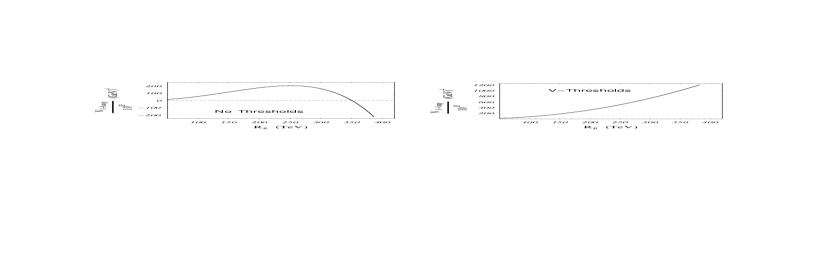
(a)                                                   (b)

FIG. 1.: The 1-loop potential as a function of the “generalized radious” $R_{g}(\phi_{1})=\sqrt{\phi_{1}^{2}+\phi_{2}^{2}}$ is shown in the $A_{0}=-400$ GeV, $M_{0}=60$ GeV, $M_{1/2}=200$ GeV and $\tan\beta=2$ case. $(\phi_{1},\phi_{2}(\phi_{1}))$ is the lowest point of H-Diag direction at an arbitrary field value $\phi_{1}={\cal H}_{1}(Q_{high})$.

FIG. 2a.: Decoupling process of the top-stops field dependent mass eigenvalues as we are moving along the line $x_{1}+x_{2}=\phi_{1}+\phi_{2}(\phi_{1})$, where $x_{i}={\cal H}_{i}$. $(\phi_{1},\phi_{2}(\phi_{1}))$ represents the lowest point of H-Diag direction when $\phi_{1}={\cal H}_{1}(Q_{high})\simeq 2\times 10^{3}$ TeV (initial conditions at $M_{X}$ same as in Fig. 1).

FIG. 2b.: Same as Fig. 2a but now for charginos and bottom-sbottoms.

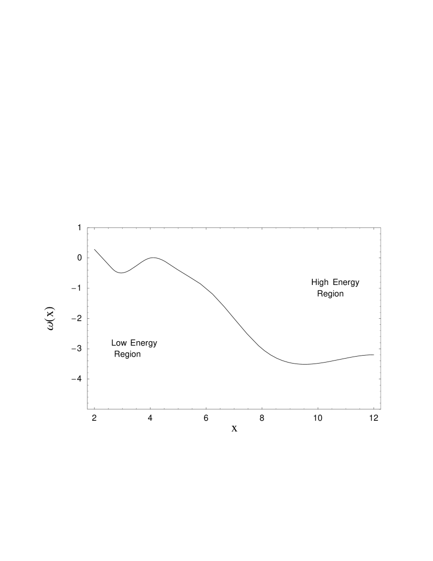
FIG. 3a.: Plot of the $\omega(x)$ used in the definition of the critical scale $\tilde{Q}^{*}$.

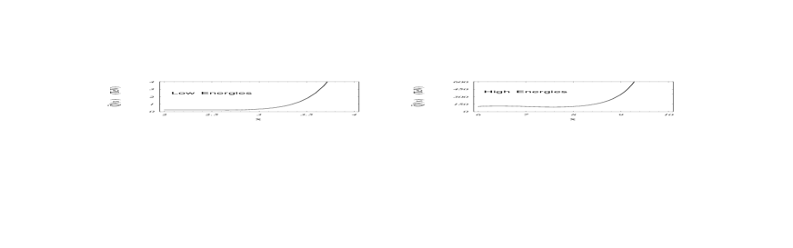
FIG. 3b.: The renormalization scale used for RG improvement of the effective potential as a function of $x={1\over 2}\log{{\cal H}_{1}^{2}+{\cal H}_{2}^{2}\over L^{2}}.$

REFERENCES

- [1] E. Gildener and S. Weinberg, Phys. Rev. D13, 3333 (1976); E. Gildener, Phys. Rev. D14, 1667 (1976); L. Susskind, Phys. Rev. D20, 2619 (1979).
- [2] For reviews see, J. Wess and J. Bagger, Supersymmetry and Supergravity (Princeton University Press, Princeton NJ, 1992); P.P. Srivastava, Supersymmetry and superfields (Adam-Hilger, Bristol England, 1986); P.G.O. Freund, Introduction to Supersymmetry (Cambridge University Press, Cambridge England, 1986); H.J.W. Müller-kirsten and A. Wiederman, Supersymmetry. An introduction with conceptual and calculational details (World Scientific, Singapore, 1987); D. Bailin and A. Love, Supersymmetric Gauge Field Theory and String Theory (Institute of Physics Publishing, Bristol England, 1994); D.R.T. Jones, “Supersymmetric gauge theories”, in TASI Lectures in Elementary Particle Physics 1984, edited by D.N. Williams (TASI publications, Ann Arbor, 1984).
- [3] For reviews see, H.E. Haber and G.L. Kane, Phys. Rep. 117, 75 (1985); A.B. Lahanas D.V. Nanopoulos, Phys. Rep. 145, 1 (1987); S.P. Martin, “A Supersymmetry Primer”, in Perspectives on Supersymmetry, edited by G.L. Kane (World Scientific, Singapore, 1998) and references therein.
- [4] J.A. Casas, A. Lleyda and C. Muñoz, Nucl. Phys. B471, 3 (1996) and references therein.
- [5] M.B. Einhorn and D.R.T. Jones, Nucl. Phys. B230 [FS10], 261 (1984); K. Nishijima, Prog. Theor. Phys. 88, 993 (1992); 89, 917 (1993); C. Ford and C. Wiesendanger, Phys. Rev. D55, 2202 (1997); Phys. Lett. B398, 342 (1997).
- [6] M. Sher, Phys. Rep. 179, 274 (1989).
- [7] M. Bando, T. Kugo, N. Maekawa and H. Nakano, Phys. Lett. B301, 83 (1992).
- [8] M. Bando, T. Kugo, N. Maekawa and H. Nakano, Prog. Theor. Phys. 90, 405 (1993); C. Ford, Phys. Rev. D50, 7531 (1994).
- [9] H. Nakano and Y. Yoshida, Phys. Rev. D49, 5393 (1994).
- [10] J.A. Casas, V. Di Clemente and M. Quiros, Report No. IEM–FT–181/98 (hep-ph 9809275).
- [11] K. Symanzik, Comm. Math. Phys. 34, 7 (1973); T. Appelquist and J. Carazzone, Phys. Rev. D11, 2856 (1975).
- [12] L. Girardello and M.T. Grisaru, Nucl. Phys. B194, 65 (1982).
- [13] For reviews see, H.P. Nilles, Phys. Rep. 110, 1 (1984); P. Nath, R. Arnowitt and A. Chamseddine, “Applied Supergravity” (World Scientific, Singapore, 1984); R. Arnowitt and P. Nath, Lectures at VII J.A. Swieca Summer School, Campos do Jordao, Brazil, 1993, Texas A&M University Report No. CTP–TAMU–52–93 (hep-ph 9309277).
- [14] M.B. Green, J.H. Schwarz and E. Witten, Superstring Theory (Cambridge University Press, Cambridge England, 1987); J. Polchinski, String theory (Cambridge University Press, Cambridge England, 1998).
- [15] J. Ellis, S. Ferrara and D. V. Nanopoulos, Phys. Lett. 114B, 231 (1982); W. Büchmuller and D. Wyler, Phys. Lett. 121B, 321 (1983); J. Polchinski and M. B. Wise, Phys. Lett. 125B, 393 (1983); F. del Aguila, M. B. Gavela, J. A. Grifols and A. Mendez, Phys. Lett. 126B, 71 (1983); S. Bertolini and F. Vissani, Phys. Lett. B324, 164 (1994); S. Abel, W. Cottingham and I. Whittingham, Phys. Lett. B370, 106 (1996); S. Khalil and Q. Shafi, Report No. BA–99–40 (hep-ph 9904448).
- [16] P. Ginsparg, Phys. Lett. 197B, 139 (1987); V. Kaplunovsky, Nucl. Phys. B307, 145 (1988); B382, 436 (1992); K. Dienes and A. Faraggi, Phys. Rev. Lett. 75, 2646 (1995); Nucl. Phys. B457, 409 (1995). For a review see, K. Dienes, Phys. Rep. 287, 447 (1997) and references therein.
- [17] K. Inoue, A. Kakuto, H. Komatsu and S. Takeshita, Prog. Theor. Phys. 68, 927 (1982); 71, 96 (1984).
- [18] S. Coleman and E. Weinberg, Phys. Rev. D9, 1888 (1973); R. Jackiw, Phys. Rev. D9, 1686 (1974).
- [19] B. Kastening, Phys. Lett. B283, 287 (1992).
- [20] S. Kelley, J. Lopez, D. Nanopoulos, H. Pois and K. Yuan, Nucl. Phys. B398, 3 (1993).
- [21] C. Ford, D.R.T. Jones, P.W. Stephenson and M.B. Einhorn, Nucl. Phys. B395, 17 (1993).
- [22] L.E. Ibañez and G.G. Ross, Phys. Lett. 110B, 215 (1982); L. E. Ibañez and C. E. Lopez, Phys. Lett. 126B, 54 (1983); Nucl. Phys. B233, 511 (1984); L. E. Ibañez, Nucl. Phys. B218, 514 (1983); L. Alvarez-Gaumé, J. Polchinski and M. Wise, Nucl. Phys. B221, 495 (1983); J. Ellis, J.S. Hagelin, D.V. Nanopoulos and K. Tamvakis, Phys. Lett. 125B, 275 (1983); L. Alvarez-Gaumé, M. Claudson and M. Wise, Nucl. Phys. B207, 96 (1982); C. Kounnas, A. B. Lahanas, D. V. Nanopoulos and M. Quiros, Phys. Lett. 132B, 95 (1982); Nucl. Phys. B236, 438 (1984).
- [23] W. Siegel, Phys. Lett. 84B, 193 (1979); D. M. Capper et al., Nucl. Phys. B167, 479 (1980); I. Antoniadis, C. Kounnas and K. Tamvakis, Phys. Lett. B119, 377 (1982); S. P. Martin and M. T. Vaughn, Phys. Lett. B318, 331 (1993).
- [24] A. Dedes, A.B. Lahanas and K. Tamvakis, Phys. Rev. D53, 3793 (1996).
- [25] S. P. Martin and M. T. Vaughn, Phys. Rev. D50, 2282 (1994). For 2-loop anomalous dimensions see P.M. Ferreira, I. Jack and D.R.T. Jones, Phys. Lett. B387, 80 (1996); B.C. Allanach, A. Dedes and H.K. Dreiner, Report No. DAMTP-1999-20 (hep-ph 9902251).
- [26] J. Yang, A note on the Higgs particles (hep-ph 9902264) and references therein.
- [27] C. Le Mouël and G. Moultaka, Nucl. Phys. B518, 3 (1998).
- [28] G. Gamberini, G. Ridolfi and F. Zwirner, Nucl. Phys. B331, 331 (1990).
- [29] B. de Carlos and J.A. Casas, Phys. Lett. B309, 320 (1993).
- [30] D.J. Castaño, E.J. Piard and P. Ramond, Phys. Rev. D49, 4882 (1994).
- [31] For a description of Adams methods see in Modern numerical methods for ordinary differential equations, edited by G. Hall and J.M. Watt (Clarendon Press, Oxford, 1976).
- [32] M. Olechowski and S. Pokorski, Nucl. Phys. B404, 590 (1993); V. Barger, M. Berger and P. Ohmann, Phys. Rev. D49, 4908 (1994); G. Kane, C. Kolda, L. Roszkowski and J. Wells, Phys. Rev. D49, 6173 (1994); W. de Boer, R. Ehret and D. Kazakov, Z. Phys. C67, 647 (1995).
- [33] Review of Particle Physics C. Caso et al., Eur. Phys. J. C3, 1 (1998).
- [34] N. Polonsky, Report No. UPR-0641-T (unpublished).
- [35] H. Arason, D. J. Castaño, B. Kesthelyi, S. Mikaelian, E. J. Piard, P. Ramond and B. D. Wright, Phys. Rev. D46, 3945 (1992).
- [36] A. Dedes, A.B. Lahanas, J. Rizos and K. Tamvakis, Phys. Rev. D55, 2955 (1997).
- [37] P.H. Chankowski, Phys. Rev. D41, 2877 (1990); M. Bando, N. Maekawa, H. Nakano and J. Sato, Mod. Phys. Lett. A8, 2729 (1993).
- [38] D.G. Papageorgiou, I.N. Demetropoulos and I.E. Lagaris, Comput. Phys. Commun. 109, 227 (1998); 109, 250 (1998).
- [39] D.V. Gioutsos and C.E. Vayonakis in preparation.
- [40] R. Arnowitt and P. Nath, Phys. Rev. D46, 3981 (1992).
- [41] S. Martin and P. Ramond, Phys. Rev. D48, 5365 (1993).
- [42] J. Stoer and R. Bulirsch, Introduction to numerical analysis (Springer–Verlag, New York, 1980).
- [43] J.H. Wilkinson, Rounding errors in algebraic processes (Dover Publications, INC., New York, 1994).
-
[44]
D. Goldberg, ACM Computing Surveys 23, 5 (1991);
See also http://metalab.unc.edu/pub/languages/fortran/unfp.html - [45] W. Press, B. Flannery, S. Teukolsky and W. Vetterling, Numerical Recipes - The Art of Scientific Computing. Second edition (Cambridge University Press, Cambridge England, 1992).
- [46] C. Reinsch and J.H. Wilkinson, “Linear Algebra”, in Vol. II of Handboook for automatic computation, edited by F.L. Bauer et al. (Springer–Verlag, New York, 1971).
- [47] W. Murray, “Failure, the causes and cures”, in Numerical methods for unconstraint optimization, edited by W. Murray (Academic Press, New York, 1972).