Quark-mass effects for jet production in $e^{+}e^{-}$ collisions at the next-to-leading order: results and applications

Abstract

We present a detailed description of our calculation of next-to-leading order QCD corrections to heavy quark production in $e^{+}e^{-}$ collisions including mass effects. In particular, we study the observables $R_{3}^{b\ell}$ and $D_{2}^{b\ell}$ in the E, EM, JADE and DURHAM jet-clustering algorithms and show how one can use these observables to obtain $m_{b}(m_{Z})$ from data at the $Z$ peak.

FTUV/99-2

, and

PACS number(s): 12.15.Ff,12.38.Bx,13.87.Ce,14.65.Fy
Keywords: $e^{+}e^{-}$ collider physics, bottom-quark mass, QCD jets, radiative corrections

1 Introduction

The origin of fermion masses is one of the unresolved puzzles in present high energy physics. To be able to answer this question one needs to know the values of the quark masses with high accuracy. However, due to confinement, quarks do not appear as free particles in nature, and therefore, the definition of their mass is ambiguous. Quark masses can be understood more easily if they are interpreted like coupling constants rather than fixed inertial parameters and, therefore, quark masses can run if measured at different scales. Moreover, in the standard model (SM) all fermion masses come from Yukawa couplings and those also run with the energy. This has very important phenomenological consequences in Higgs boson searches since the parameter that governs the decay rate of the Higgs boson to bottom quarks [1, 2, 3] is the running mass of the $b$-quark at the $m_{H}$ scale, $m_{b}(m_{H})$, which is much smaller than the quark mass extracted at threshold. On the other hand, from the model building point of view, to test fermion mass models one has to run masses extracted at quite different scales up to the same scale and compare them with the same “ruler” [4]. This way, for instance, one can check that, in some grand unified models, although the $b$-quark mass and the tau mass are very different at threshold energies, they could be equal at the unification scale [5, 6].

However, although predicted by quantum field theory, the possibility of testing experimentally the running of fermion masses has not been considered until very recently [6, 7, 8, 9, 10, 11, 12, 13, 14]. The reason being that for energies much higher than the fermion mass the mass effects become negligible for most observables. In principle, it is clear that the running of quark masses will be checked, once the Higgs is discovered, by measuring directly the Yukawa couplings in Higgs decays. We think it is also interesting to explore the possibility of measuring quark masses far away from threshold in order to check the running.

In [7, 15, 16, 17, 18] it was shown that mass effects in three-jet production at the $Z$ peak are large enough to be measured but in [7] we also showed that a next-to-leading order (NLO) calculation of three-jet ratios including mass effects was necessary in order to extract a meaningful value for the $b$-quark mass. This is because the leading order (LO) calculation does not distinguish among the different quark mass definitions (e.g. perturbative pole mass or $\overline{\mathrm{MS}}$ running mass).

Although jet production of heavy quarks has been considered in a large variety of processes, there are very few NLO calculations of jet production taking into account complete mass effects. In [19] those were calculated for gluon-gluon fusion in proton-antiproton collisions, while in [20] the complete NLO corrections were computed for virtual-photon production of heavy quarks in deep-inelastic electron-proton scattering. However, until very recently, no full calculation of jet production of heavy quarks in $e^{+}e^{-}$ collisions was available at NLO. In [8, 12] we have presented the final results of such a calculation and have shown how can one use the DURHAM ($k_{T}$) clustering algorithm to extract the $b$-quark mass at the $m_{Z}$ scale. Finally in [14] the DELPHI collaboration has presented the measurement of $m_{b}(m_{Z})$. The obtained value is in good agreement with low energy measurements and running of the mass from $\mu=m_{b}$ to $\mu=m_{Z}$ as predicted by QCD with 5 flavours. Our NLO calculation was also used in [14] to check the universality of the strong interactions. In the meanwhile two more groups, ref. [36, 37] and ref. [38, 39, 40, 41], have also presented NLO results of jet production of heavy quarks in $e^{+}e^{-}$ collisions by using different calculational schemes. On the other hand also the different experimental collaborations have started to use NLO calculations of mass effects in order to check the universality of the strong interactions [42, 43, 44] and have also shown that mass effects are absolutely necessary to explain the data.

In this paper we present a detailed description of our calculation of the NLO corrections to the rates of jet production of massive quarks in $e^{+}e^{-}$ collisions for the different jet-clustering algorithms discussed in [7]. In [14, 12] only the DURHAM algorithm was used because it has a very good behaviour from both the experimental and the theoretical points of view. It is important to stress that not all the observables are equally good to study mass effects. In particular observables which suffer from huge NLO corrections cannot be used to extract any reasonable value of the $b$-quark mass.

Although, in principle, we will concentrate on $b$-quark production at the $Z$-peak, some of the results can also be applied to $t$-$\bar{t}$ production at the NLC (Next-Linear-Collider).

In section 2 we review the leading order results, give LO amplitudes in $D$-dimensions and introduce the jet-clustering algorithms we use. In section 3 the strategy of the NLO calculation in the framework of the phase-space slicing method [45, 46, 47, 48, 49, 50, 51] is explained. Section 4 gives all the contributions coming from three partons, while in section 5 we give all four-parton contributions and show the cancellation of the infrared (IR) divergences among three-parton and four-parton contributions. Finally in section 6 we present numerical results for the finite parts and review applications of this calculation. In particular we study two observables, $R_{3}^{b\ell}$ (the ratio of the three-jet rate containing the $b$-quark to the three-jet rate of light quarks) and $D_{2}^{b\ell}$ (the ratio of the differential two-jet rate containing the $b$-quark to the differential rate of light quarks), computed in the different jet-clustering algorithms and show how they can be used to extract $m_{b}(m_{Z})$ from data at the $Z$-peak. In the appendices we collect some of the formulae used in the main calculation. Thus, in appendix A we give the most relevant one-loop scalar functions that appear in the calculation of the virtual corrections. In appendix B we review the calculation of phase-space in D-dimensions. Finally in appendix C we collect some of the IR divergent integrals which appear in the calculation of four-parton contributions.

2 The decay $Z\rightarrow 3jets$ with heavy quarks at the leading order

2.1 Decay into two and three jets and jet-clustering algorithms

The lowest order contribution to the $Z$-boson decay into three jets in the parton picture is given by the decay $Z\rightarrow b\bar{b}g$. This partonic process has an infrared singularity because a massless gluon could be radiated with zero energy. It is well known [52, 53, 54], however, that this divergence is exactly canceled by the IR-divergent part of the two-parton decay width of the $Z$-boson, $Z\rightarrow b\bar{b}$, at the order ${\cal{O}}(\alpha_{s})$. In the last process the IR divergence occurs due to massless gluons running in the loops.

Thus, in order to define IR-finite observables, we need to introduce some resolution parameter, $y_{c}$, and to split the full three-parton phase-space into the two-jet region, containing soft gluon emission, and the remaining three-jet region. The sum of the three-parton decay probability integrated over the two-jet part of the phase-space and the two-parton decay width at the order ${\cal{O}}(\alpha_{s})$ defines the IR finite two-jet decay width, $\Gamma^{b}_{2j}$, at the next-to-leading order. The integration over the rest of the three-parton phase-space gives the three-jet decay width, $\Gamma^{b}_{3j}$, at the leading order and it is also IR finite.

Although both IR-finite $\Gamma^{b}_{2j}(y_{c})$ and $\Gamma^{b}_{3j}(y_{c})$ depend on the resolution parameter, it is obvious that the sum of the two-jet and three-jet decay widths is independent of $y_{c}$ and is given by the total (inclusive) decay width of the $Z$-boson into the heavy quarks at the next-to-leading order:

$$\Gamma^{b}=\Gamma^{b}_{2j}(y_{c})+\Gamma^{b}_{3j}(y_{c})~{}.$$

Therefore, at order ${\cal{O}}(\alpha_{s})$, knowing $\Gamma^{b}$ and $\Gamma^{b}_{3j}(y_{c})$ we can obtain $\Gamma^{b}_{2j}(y_{c})$ as well. The analytical expression for the $\Gamma^{b}$ with quark-mass corrections can be found in [7, 25, 26, 55, 56, 57].

In the same way, at the next-to-next-to-leading order we can write for the total width:

$$\Gamma^{b}=\Gamma^{b}_{2j}(y_{c})+\Gamma^{b}_{3j}(y_{c})+\Gamma^{b}_{4j}(y_{c})~{}.$$ (2.1)

Now the four-jet decay width, $\Gamma^{b}_{4j}(y_{c})$, receives contributions from four-parton processes. The three-jet decay width, $\Gamma^{b}_{3j}(y_{c})$, gets contributions from order ${\cal O}(\alpha_{s}^{2})$ one-loop corrected three-parton processes and the soft part of the four-parton processes such that the sum is IR-finite. Thus, knowing $\Gamma^{b}$, $\Gamma^{b}_{3j}(y_{c})$ and $\Gamma^{b}_{4j}(y_{c})$ we can obtain $\Gamma^{b}_{2j}(y_{c})$ at order ${\cal O}(\alpha_{s}^{2})$.

Let us discuss now the definition of jets in more detail. The most popular jet definitions used in the analysis of the $e^{+}e^{-}$-annihilation during the last years are based on the so-called jet-clustering algorithms. These algorithms have to be applied to define jets in both, the theoretical calculations at the parton level, and in the analysis of the bunch of real particles observed at experiment.

In the jet-clustering algorithms jets are usually defined as follows: starting from a bunch of $n$ particles with four-momenta $p_{i},~{}(i=1..n)$ one computes a resolution function depending on the momenta of two particles, for example,

$$y_{ij}=2\frac{E_{i}E_{j}}{s}(1-\cos\theta_{ij})~{},$$

for all pairs $(i,~{}j)$ of particles. Then one takes the minimum of all $y_{ij}$ and, if it satisfies that it is smaller than a given quantity $y_{c}$ (the resolution parameter, y-cut), the two particles which define the minimal $y_{ij}$ are regarded as belonging to the same jet. Then they are recombined into a new pseudo-particle with the four-momentum defined according to some rule, for example,

$$p_{k}=p_{i}+p_{j}~{}.$$

After this first step one has a bunch of $n-1$ (pseudo)particles and the algorithm is applied again and again until all the remaining (pseudo)particles satisfy the criteria $y_{ij}>y_{c}$. The final number of (pseudo)particles is the number of jets in the considered event and the momenta of the (pseudo)particles define the event kinematics.

In theoretical calculations one can define a jet cross-section or a decay width into jets as a function of $y_{c}$, which are computed at the parton level, by following exactly the algorithm described above. Jet-clustering algorithms lead automatically to IR finite quantities. Furthermore, it has been shown in the literature, using Monte Carlo models, that, for some of the algorithms, the passage from partons to hadrons (hadronization) does not change much the behaviour of the jet-observables [61], thus allowing to compare theoretical predictions with experimental results. We refer to [61, 62] for a detailed discussion and comparison of different successful jet-clustering algorithms used in $e^{+}e^{-}$ annihilation in the case of massless quarks. Hadronization corrections for the case of massive quarks have also been studied for the DURHAM algorithm [14].

In this paper we will present results and compare them for the four jet-clustering algorithms listed in table 1, where $\sqrt{s}$ is the total center of mass energy. Already in ref. [7] we showed that the $E$-algorithm has a very peculiar behaviour when massive partons are involved. It is because for the same values of particle momenta, the resolution function, $y_{ij}$, is significantly shifted, comparing with the massless case, when the quark masses are included. To avoid these problems in the massive case we introduced in ref. [7] the $EM$-algorithm, which is similar to the $E$-algorithm. As mentioned above, all observables have a completely different dependence on $y_{c}$ for the $E$-algorithm and this can serve as a good test of both calculations and data analyses. The application of the new interesting Cambridge algorithm [58, 59, 60] in the massive case is presently under study [63, 64, 65, 66, 67].

Table 1: The jet-clustering algorithms

Algorithm	Resolution function, $y_{ij}$	Combination rule
EM	$2(p_{i}\cdot p_{j})/s$	$p_{k}=p_{i}+p_{j}$
JADE	$2E_{i}E_{j}(1-\cos\theta_{ij})/s$	$p_{k}=p_{i}+p_{j}$
E	$(p_{i}+p_{j})^{2}/s$	$p_{k}=p_{i}+p_{j}$
DURHAM	$2\min(E_{i}^{2},E_{j}^{2})(1-\cos\theta_{ij})/s\ \$	$p_{k}=p_{i}+p_{j}$

It is convenient to parameterize the final IR-finite result for the three-jet decay width of the $Z$-boson in the following general form ($D=4$):

$$\Gamma^{b}_{3j}=\sqrt{s}\frac{\alpha}{64s_{W}^{2}c_{W}^{2}}\frac{\alpha_{s}}{\pi}\left[g_{V}^{2}(b)H_{V}(y_{c},r_{b})+g_{A}^{2}(b)H_{A}(y_{c},r_{b})\right]~{},$$ (2.2)

where the functions $H_{V(A)}(y_{c},r_{b})$ depend, obviously, on what jet-clustering algorithm has been used to define the three-jet region of phase-space. We have introduced the notation $r_{b}=M_{b}^{2}/s$, where $s=m_{Z}^{2}$ for the $Z$-decay. Here and in the following $M_{b}$ will stand for the perturbative pole mass of the $b$-quark, while the running mass will be denoted as $m_{b}(\mu)$. The vector and axial-vector neutral-current couplings $g_{V}(f)$ and $g_{A}(f)$ of a fermion, $f$, in the Standard Model are given by

$$g_{V}(f)=2T^{3}_{f}-4Q_{f}s^{2}_{W},\qquad g_{A}(f)=-2T^{3}_{f},$$ (2.3)

being $s_{W}~{}(c_{W})$ the sine (cosine) of the weak mixing angle, $T^{3}_{f}$ the third component of the weak isospin and $Q_{f}$ the electric charge of the fermion.

We can expand the $H_{V(A)}$ functions in the strong coupling constant, $\alpha_{s}$

$$H_{V(A)}(y_{c},r_{b})=H^{(0)}_{V(A)}(y_{c},r_{b})+\frac{\alpha_{s}}{\pi}H^{(1)}_{V(A)}(y_{c},r_{b})+\cdots~{},$$ (2.4)

where $H^{(0)}_{V(A)}$ and $H^{(1)}_{V(A)}$ are the LO and NLO contributions, respectively. Furthermore, in order to see more clearly the size of quark-mass effects, when the masses are small with respect to the center of mass energy, we found it convenient to rewrite these functions factoring the dominant $r_{b}$-dependence

$$H^{(i)}_{V(A)}(y_{c},r_{b})\equiv A^{(i)}_{V(A)}(y_{c})+{r_{b}}B^{(i)}_{V(A)}(y_{c},r_{b})~{}.$$ (2.5)

Note that eq. (2.5) is not an expansion in $r_{b}$ because the functions $B^{(i)}_{V(A)}(y_{c},r_{b})$ contain the exact residual $r_{b}$-dependence.

In the limit of zero quark masses, $r_{b}=0$, chirality is conserved and the two lowest-order functions $H^{(0)}_{V}(y_{c},r_{b})$ and $H^{(0)}_{A}(y_{c},r_{b})$ become identical

$$H^{(0)}_{V}(y_{c},0)=H^{(0)}_{A}(y_{c},0)\equiv A^{(0)}(y_{c})~{}.$$ (2.6)

This is not true at the NLO where the vector and the axial-vector functions, $A^{(1)}_{V}$ and $A^{(1)}_{A}$, are not equal anymore due to the small contribution of the triangle diagram [68] $V12$ in fig. 2.

The LO and NLO massless contributions, the $A^{(0)}$ and $A^{(1)}_{V}$ functions, were calculated in [61] using the results from [69]. In [7] the lowest order mass effects, functions $B^{(0)}_{V(A)}$, have been calculated analytically for the EM jet-clustering algorithm and numerically for JADE, DURHAM and E algorithms. For completeness, we review in the next section the LO results. Results for the NLO heavy quark contribution, in particular the functions $B^{(1)}_{V(A)}$ in eq. (2.5) will be presented later.

Concluding this section we would like to make the following remark. In this paper we discuss the $Z$-boson decay. In LEP experiments one studies the process $e^{+}e^{-}\rightarrow(Z\gamma^{*})\rightarrow b\bar{b}+\cdots$ and, apart from the resonant $Z$-exchange cross-section, there are contributions from the pure $\gamma$-exchange and from the $\gamma-Z$-interference. The non-resonant $\gamma$-exchange contribution at the peak is less than 1% for muon production and in the case of $b$-quark production there is an additional suppression factor $Q_{b}^{2}=1/9$. In the vicinity of the $Z$-peak the interference is also suppressed because it is proportional to $Q_{b}(s-m_{Z}^{2})$. However, away from the $Z$ resonance these contributions are important and should be properly taken into account.

The extension of our calculation for the cross-section of $e^{+}e^{-}$ annihilation into three jets can be done [55] as follows

$$\sigma^{b}_{3j}(s,y_{c},r_{b})=\frac{\alpha_{s}}{\pi}\left[\sigma^{b}_{V}(s)H_{V}(y_{c},r_{b})+\sigma^{b}_{A}(s)H_{A}(y_{c},r_{b})\right]$$

with the same $H_{V(A)}(y_{c},r_{b})$ functions introduced in eq. (2.2) for the Z-decay. The functions $\sigma^{b}_{V(A)}(s)$ have the form ($D=4$):

$$\sigma^{b}_{V}(s)=\frac{4\pi\alpha^{2}}{s} \left\{Q_{e}^{2}Q_{b}^{2}+2Q_{e}Q_{b}\frac{1}{16s_{W}^{2}c_{W}^{2}}g_{V}(e)g_{V}(b)Re(\chi(s))\right.$$

$$+\left.\frac{1}{64s_{W}^{4}c_{W}^{4}}g_{V}(b)^{2}\left[g_{V}(e)^{2}+g_{A}(e)^{2}\right]|\chi(s)|^{2}\right\}~{},$$

$$\sigma^{b}_{A}(s)=\frac{4\pi\alpha^{2}}{s} \left\{\frac{1}{64s_{W}^{4}c_{W}^{4}}g_{A}(b)^{2}\left[g_{V}(e)^{2}+g_{A}(e)^{2}\right]|\chi(s)|^{2}\right\}~{},$$ (2.7)

where

$$\chi(s)=\frac{s}{s-m_{Z}^{2}+im_{Z}\Gamma_{Z}~{}}.$$

Also, the numerically important QED initial-state radiation (ISR) should be taken into account in the realistic analysis of the experimental data. The cross-section of the three-jet production including ISR can be written as a convolution

$$\tilde{\sigma}^{b}_{3j}(s,y_{c},r_{b})=\int\sigma^{b}_{3j}(s^{\prime},y_{c},r_{b})F_{ISR}(s^{\prime}/s)ds^{\prime}~{},$$ (2.8)

where $F_{ISR}(s^{\prime}/s)$ is the well-known QED radiator [70] for the total cross-section and $s^{\prime}$ denotes the invariant mass of the jet final state.

2.2 $Z\rightarrow 3jets$ at tree level

In the NLO calculation of the $Z$-decay width into three-jets, which will be presented in the next sections, we encounter ultraviolet (UV) and infrared singularities. We use dimensional regularization to regularize both types of divergences and therefore most of the calculation has to be done in arbitrary $D$-dimensions. The calculation of $\Gamma^{b}_{3j}(y_{c})$ at order $\alpha_{s}$ is a pure tree-level calculation and it does not have any IR problem, since the soft gluon region is excluded from the three-parton phase-space. Therefore, the calculation can be safely done in four dimensions. However, the later use of the LO results in some steps of the NLO calculation require the tree-level results in $D$-dimensions that we present in the following.

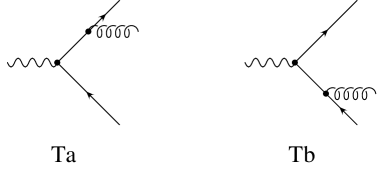
Figure 1: Tree-level diagrams contributing to $Z\rightarrow b\bar{b}g$.

In $D=4-2\epsilon$ dimensions the Born transition probability for the three-parton process, $Z\rightarrow b\ \bar{b}\ g$, summed over final colours and spins and averaged over initial spins is equal to

$$\overline{\sum}\mid M_{b\bar{b}g}\mid^{2}=\frac{g^{2}}{16c_{W}^{2}}g_{s}^{2}\frac{C_{F}N_{C}}{3-2\epsilon}\>T_{b\bar{b}g}~{},$$ (2.9)

where $g$ the $SU(2)$ coupling constant, $g_{s}$ is the strong coupling constant, $C_{F}=4/3$ and $N_{C}=3$ are $SU(3)$ group invariant factors and

$$T_{b\bar{b}g}(y_{13},y_{23}) = 16\left\{\frac{h_{p}}{y_{13}^{2}y_{23}^{2}}T_{b\bar{b}}+g_{V}^{2}(b)(1-\epsilon)\left[\frac{1}{2}(1-\epsilon)\left(\frac{y_{13}}{y_{23}}+\frac{y_{23}}{y_{13}}\right)-\epsilon\right]\right.$$ (2.10)

$$\left.\hskip-42.67912pt+g_{A}^{2}(b)(1-\epsilon)\left[\frac{1}{2}(1-\epsilon+2r_{b})\left(\frac{y_{13}}{y_{23}}+\frac{y_{23}}{y_{13}}\right)+2r_{b}-\epsilon\right]\right\}~{},$$

with

$$y_{13}=\frac{2(p_{1}\cdot p_{3})}{s}~{},\qquad y_{23}=\frac{2(p_{2}\cdot p_{3})}{s}~{},$$

where $p_{1}$, $p_{2}$ and $p_{3}$ are the four-momenta of the quark, the antiquark and the gluon, respectively. The function $h_{p}(y_{13},y_{23})$ defines the three-body phase-space boundaries (See eq. (B.3)) and the dimensionless function

$$T_{b\bar{b}}=g_{V}^{2}(b)(1-\epsilon+2r_{b})+g_{A}^{2}(b)(1-\epsilon)(1-4r_{b})~{},$$ (2.11)

is related to the Born two-parton process, $Z\rightarrow b\ \bar{b}$, transition probability through

$$\overline{\sum}\mid M_{b\bar{b}}\mid^{2}=\frac{g^{2}}{16c_{W}^{2}}\frac{N_{C}}{3-2\epsilon}\>4s\>T_{b\bar{b}}~{}.$$ (2.12)

Averaging over the $Z$-boson polarizations we took into account that in arbitrary space-time dimensions the number of spin degrees of freedom is $D-1=3-2\epsilon$.

Table 2: The leading order functions (see eqs. (2.2, 2.4, 2.5)) for the E algorithm.

$y_{c}$	$A^{(0)}\>\>$	$B^{(0)}_{V}/A^{(0)}$
		$M_{b}=3$GeV	$M_{b}=4$GeV	$M_{b}=5$GeV
0.01	18.627	37.811	39.353	42.432
0.02	12.209	22.195	21.645	21.723
0.03	9.069	16.917	16.314	15.840
0.04	7.118	13.540	13.560	13.135
0.05	5.765	11.390	11.466	11.452
0.06	4.764	9.932	9.981	10.043
0.07	3.990	8.889	8.920	8.960
0.08	3.374	8.118	8.138	8.162
0.09	2.873	7.540	7.551	7.565
0.10	2.458	7.108	7.113	7.118
$y_{c}$	$A^{(0)}\>\>$	$B^{(0)}_{A}/A^{(0)}$
		$M_{b}=3$GeV	$M_{b}=4$GeV	$M_{b}=5$GeV
0.01	18.627	32.506	33.827	36.578
0.02	12.209	17.188	16.532	16.462
0.03	9.069	12.084	11.414	10.847
0.04	7.118	8.838	8.812	8.321
0.05	5.765	6.797	6.838	6.777
0.06	4.764	5.436	5.455	5.481
0.07	3.990	4.478	4.486	4.495
0.08	3.374	3.785	3.785	3.785
0.09	2.873	3.280	3.274	3.267
0.10	2.458	2.914	2.905	2.893

Table 3: The leading order functions (see eqs. (2.2, 2.4, 2.5)) for the EM algorithm.

$y_{c}$	$A^{(0)}\>\>$	$B^{(0)}_{V}/A^{(0)}$
		$M_{b}=3$GeV	$M_{b}=4$GeV	$M_{b}=5$GeV
0.01	18.628	-18.708	-18.778	-18.444
0.02	12.209	-12.406	-13.178	-13.529
0.03	9.069	-10.081	-10.637	-11.167
0.04	7.118	-9.464	-9.480	-9.813
0.05	5.765	-9.162	-9.161	-9.168
0.06	4.764	-9.018	-9.016	-9.013
0.07	3.990	-8.973	-8.970	-8.966
0.08	3.374	-8.997	-8.993	-8.988
0.09	2.873	-9.073	-9.068	-9.062
0.10	2.458	-9.192	-9.186	-9.178
$y_{c}$	$A^{(0)}\>\>$	$B^{(0)}_{A}/A^{(0)}$
		$M_{b}=3$GeV	$M_{b}=4$GeV	$M_{b}=5$GeV
0.01	18.628	-23.675	-23.678	-23.261
0.02	12.209	-17.214	-17.931	-18.215
0.03	9.069	-14.764	-15.269	-15.736
0.04	7.118	-14.042	-14.008	-14.279
0.05	5.765	-13.648	-13.598	-13.544
0.06	4.764	-13.419	-13.370	-13.308
0.07	3.990	-13.295	-13.247	-13.184
0.08	3.374	-13.246	-13.198	-13.135
0.09	2.873	-13.255	-13.205	-13.142
0.10	2.458	-13.310	-13.260	-13.195

Table 4: The leading order functions (see eqs. (2.2, 2.4, 2.5)) for the JADE algorithm.

$y_{c}$	$A^{(0)}\>\>$	$B^{(0)}_{V}/A^{(0)}$
		$M_{b}=3$GeV	$M_{b}=4$GeV	$M_{b}=5$GeV
0.01	18.627	-34.488	-31.314	-28.526
0.02	12.209	-25.045	-24.050	-22.805
0.03	9.069	-20.158	-19.968	-19.527
0.04	7.118	-17.410	-17.308	-17.191
0.05	5.765	-15.675	-15.596	-15.501
0.06	4.764	-14.491	-14.437	-14.384
0.07	3.990	-13.613	-13.577	-13.529
0.08	3.374	-12.924	-12.902	-12.870
0.09	2.873	-12.393	-12.373	-12.346
0.10	2.458	-11.979	-11.964	-11.943
$y_{c}$	$A^{(0)}\>\>$	$B^{(0)}_{A}/A^{(0)}$
		$M_{b}=3$GeV	$M_{b}=4$GeV	$M_{b}=5$GeV
0.01	18.627	-39.412	-36.144	-33.244
0.02	12.209	-29.823	-28.753	-27.415
0.03	9.069	-24.817	-24.560	-24.035
0.04	7.118	-21.968	-21.802	-21.606
0.05	5.765	-20.142	-20.002	-19.832
0.06	4.764	-18.876	-18.764	-18.638
0.07	3.990	-17.921	-17.829	-17.711
0.08	3.374	-17.161	-17.086	-16.986
0.09	2.873	-16.564	-16.492	-16.399
0.10	2.458	-16.088	-16.022	-15.937

Table 5: The leading order functions (see eqs. (2.2, 2.4, 2.5)) for the DURHAM algorithm.

$y_{c}$	$A^{(0)}\>\>$	$B^{(0)}_{V}/A^{(0)}$
		$M_{b}=3$GeV	$M_{b}=4$GeV	$M_{b}=5$GeV
0.01	7.836	-27.862	-27.092	-26.202
0.02	5.127	-20.038	-19.800	-19.509
0.03	3.815	-16.760	-16.652	-16.517
0.04	3.003	-14.889	-14.833	-14.762
0.05	2.440	-13.659	-13.628	-13.589
0.06	2.023	-12.780	-12.764	-12.743
0.07	1.701	-12.117	-12.110	-12.101
0.08	1.443	-11.598	-11.597	-11.595
0.09	1.233	-11.180	-11.183	-11.186
0.10	1.058	-10.836	-10.842	-10.849
$y_{c}$	$A^{(0)}\>\>$	$B^{(0)}_{A}/A^{(0)}$
		$M_{b}=3$GeV	$M_{b}=4$GeV	$M_{b}=5$GeV
0.01	7.836	-32.216	-31.337	-30.316
0.02	5.127	-24.256	-23.934	-23.537
0.03	3.815	-20.880	-20.698	-20.471
0.04	3.003	-18.930	-18.807	-18.652
0.05	2.440	-17.634	-17.541	-17.423
0.06	2.023	-16.698	-16.623	-16.527
0.07	1.701	-15.985	-15.922	-15.841
0.08	1.443	-15.421	-15.366	-15.295
0.09	1.233	-14.964	-14.915	-14.851
0.10	1.058	-14.584	-14.539	-14.481

In the limit of zero energy of the emitted gluon, both invariants $y_{13}$ and $y_{23}$ approach zero and the first term in the eq. (2.10) develops an IR singularity. The IR-finite three-jet decay width of the $Z$-boson at LO is given by the integral of the transition probability $T_{b\bar{b}g}(y_{13},y_{23})$, eq. (2.10), over the three-jet region of the phase-space, where the soft-gluon region is excluded:

$$\Gamma^{b}_{3j}=\left[\frac{1}{2\sqrt{s}}\int dPS(3)\overline{\sum}\mid M_{b\bar{b}g}\mid^{2}\theta_{c}(y_{c};y_{13},y_{23})\right]_{\epsilon=0,~{}s=m_{Z}^{2}}~{}.$$ (2.13)

The function $\theta_{c}(y_{c};y_{13},y_{23})$ introduces the appropriate cuts for each of the jet-clustering algorithms and defines the three-jet region.

At the lowest order, E, JADE and EM give the same three-jet rates for massless particles, because in this case there is no parton recombination involved and all the three schemes have the same resolution parameter. However, already at order $\alpha_{s}^{2}$ they give different results since after the first recombination the pseudo-particles are not massless anymore and the resolution functions are different. For massive quarks the three algorithms, E, JADE and EM are already different at order $\alpha_{s}$. The DURHAM algorithm is, of course, completely different from the other algorithms we use, both in the massive and the massless cases.

Tables 2, 3, 4 and 5 present the dependence of the function $A^{(0)}(y_{c})$ and the ratio of functions $B^{(0)}_{V(A)}(y_{c},r_{b})/A^{(0)}(y_{c})$ on the jet-resolution parameter $y_{c}$ for the different jet schemes and for several relevant values of $M_{b}$. It is clearly seen from the tables that both leading order functions $B^{(0)}_{V}$ and $B^{(0)}_{A}$ have a soft dependence on $M_{b}$ for the region of y-cut, $y_{c}\geq 0.01$, which is relevant for experimental studies.

3 Three-jet ratios at next-to-leading order: overview of the calculation

Like for many QCD processes it turns out that the leading order calculation of the $Z$-boson decay into three-jets, described in the previous section, does not match the experimental precision. The numerical results for the leading order calculation were presented in [33, 34, 7] (see also section 2.2). It is known [61] that next-to-leading corrections to the decay of the $Z$-boson into massless quarks are very significant numerically. In addition, at the leading order we do not have any idea what value of the quark mass should be taken. The various perturbative definitions of the quark mass (pole mass, running mass etc.) differ only at the next-to-leading order. However, the numerical difference when several mass definitions are used in the leading order prediction for three-jet observables is large [7]. It is again an indication that next-to-leading corrections are important. Therefore, to use consistently the quark mass definition, and to provide accurate predictions for three-jet observables, the next-to-leading order, ${\cal O}(\alpha_{s}^{2})$, calculation for massive quarks has to be included.

The main difficulty of the NLO calculation is the appearance at the intermediate stages, in addition to ultraviolet divergences, of infrared and collinear singularities due to massless gluons. The Bloch-Nordsieck and Kinoshita-Lee-Nauenberg theorems [52, 53, 54] assure, however, that observable jet cross-sections are infrared finite and free from collinear divergences.

At the NLO the three-jet cross-section has contributions from three-parton, figs. 2 and 3, and four-parton, figs. 5, 6 and 7, final states.

The IR and collinear singularities of the NLO one-loop Feynman diagrams cancel against divergences that appear when the differential cross-section for four-parton production is integrated over the region of phase-space where either one gluon is soft or two gluons are collinear. However, the singularities that appear in the intermediate steps of the calculation should be treated properly. We used dimensional regularization to regularize both UV and IR divergences [71, 72, 73] because this regularization preserves the QCD Ward identities.

The three-parton transition amplitude can be expressed in terms of a few scalar one-loop integrals. The result contains poles in $\epsilon=(4-D)/2$, where $D$ is a space-time dimension. Some of the poles have UV origin and other correspond to the IR singularities. All UV divergences are removed by appropriate renormalization of the parameters of the QCD Lagrangian (coupling constant, mass and wave functions). After UV renormalization and taking the interference with the tree-level three-parton amplitude we obtain analytical expressions which have a part containing the IR poles (single and double) and a finite contribution. The singular part is proportional to the leading order transition probability.

The four-parton transition probabilities are split in two parts. The first one, the so-called soft part, contains singularities when one of the massless partons in the final state is soft, or two massless final partons are collinear. The second part, denoted as hard, is free from any potential singularities. Then, to cancel the IR/collinear divergences against those appearing in the three-parton contribution we work in the context of the phase-space slicing method [45, 46, 47, 48, 49, 50, 51]. In this method the analytical integration over a thin slice at the border of the phase-space, which contains the IR/collinear singularities, is performed in $D$-dimensions by using approximate expressions for the transition probability expanded in the slice-parameter that defines the size of the slice. The result is added to the virtual corrections. The sum becomes free of singularities and can be integrated numerically for $D=4$ in the three-jet region of the three-body phase-space (defined by the jet-clustering algorithms considered in the previous section: EM, JADE, E and DURHAM), but it depends on the small slice-parameter. The integration of the hard part over the three-jet region of the four-body phase-space (again defined by the jet-clustering algorithms considered above) is done numerically for $D=4$.

The sum of the three-parton and four-parton contributions to the three-jet decay width of the $Z$ boson should be independent of the parameter that defines the slice as long as it is small enough not to spoil the approximations used. The independence of this parameter has been checked in our calculations. Finally, we obtain the finite functions $H_{V}(y_{c},r_{b})$ and $H_{A}(y_{c},r_{b})$ in eq. (2.5) at order $\alpha_{s}$.

Our classification of the transition probabilities is similar to the one used by Ellis, Ross and Terrano [69] which is based on a colour factor classification. The way the cancellation of IR divergences occurs can be seen by representing the different transition probabilities as the different cuts one can perform in the three-loop bubble diagrams contributing to the $Z$-boson selfenergy. Therefore, we assign both three- and four-parton transition probabilities to the different classes defined by the six bubble diagrams depicted in fig 4. The advantage of this classification is that the cancellation of IR divergences occurs for each class of diagrams separately and, therefore, numerical tests can be performed independently for the IR finite result obtained in each class.

4 Three-parton contributions

4.1 Classification of diagrams

The complete set of diagrams describing the one-loop radiative corrections to the process

$$Z(q)\rightarrow b(p_{1})+\bar{b}(p_{2})+g(p_{3})~{},$$ (4.1)

is shown in figs. 2 and 3. They contribute to the three-jet decay rate at $O(\alpha_{s}^{2})$ through their interference with the lowest order bremsstrahlung diagrams $Ta$ and $Tb$ in fig. 1.

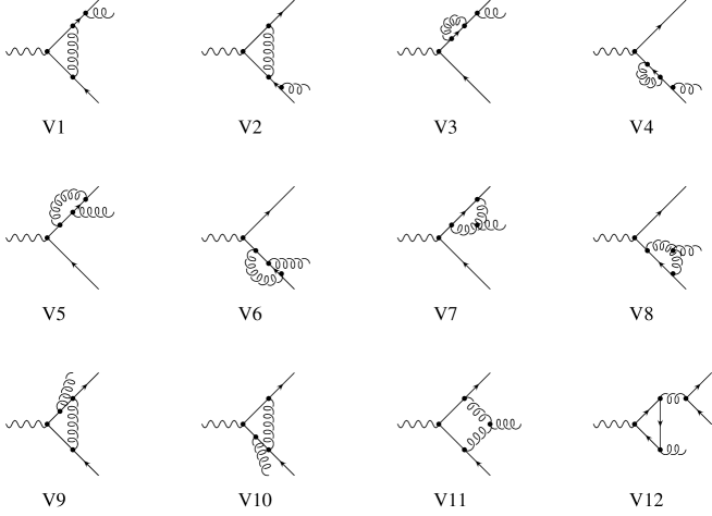
Figure 2: Radiative corrections to the process $Z\rightarrow b\bar{b}g$. Diagrams $V1$ to $V12$ contribute at $O(\alpha_{s}^{2})$ through their interference with the lowest order bremsstrahlung diagrams $Ta$ and $Tb$.

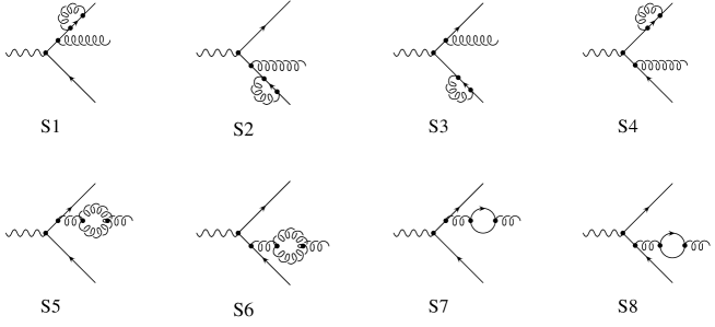
Figure 3: Selfenergy diagrams. Graphs involving ghosts and similar in structure to $S5$ and $S6$ have not been shown.

We denote by $Via$ and $Sja$ the interference of diagrams $Vi$ and $Sj$ with $Ta$ averaged (summed) over initial (final) colours and spins,

$$Via=\overline{\sum}Re\{Vi*Ta^{+}\},\qquad Sja=\overline{\sum}Re\{Sj*Ta^{+}\}~{}.$$ (4.2)

Interference with $Tb$ is denoted in the same way by $Vib$ and $Sjb$.

As usual in QCD calculations in the $\overline{\mathrm{MS}}$ scheme at LEP energies, we are working in a theory with $N_{F}=5$ quark flavours in which only the $b$-quark is considered massive. Therefore, in all closed quark loops in fig. 3 all five quarks are running in the loop. The contribution of the triangle diagram V12 in fig. 2 is peculiar. This contribution is due entirely to the fact that the top-quark and the bottom-quark are not degenerated [68] (lighter quarks are effectively degenerated), thus, both top and bottom quarks are kept in the loop.

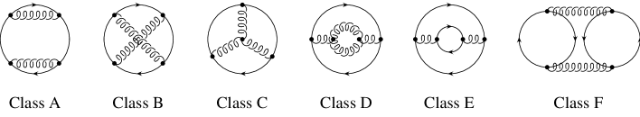
Figure 4: Bubble classification relating virtual and real contributions at $O(\alpha_{s}^{2})$ according to their divergent structure. Again we do not show diagrams similar to Class D with ghosts in the loop.

It turned out very convenient to classify the different one-loop three-parton as well as four-parton contributions based on the six three-loop bubble diagrams presented in fig. 4. Different cuts of the same diagram represent either a tree-level four-parton transition probability, or a one-loop three-parton transition probability, or a two-loop two-parton transition probability. Contributions, corresponding to different bubble diagrams are proportional to different colour factors. Then, the cancellation of IR divergences occurs separately between contributions obtained from the same class of diagrams.

The classification of all one-loop contributions to the decay $Z\rightarrow\bar{b}bg$ is shown in table 6. In every column of the table we group contributions with the same colour factor which is shown above the column. Here $T_{R}=1/2$. The transition probabilities in the third and the fourth rows of the table can be obtained from the ones in the first and second rows by the interchange of the quark and antiquark momenta.

Table 6: The interchange table relating the graphs for $Z\rightarrow b\bar{b}g$. The third and the fourth rows are obtained from the first and the second rows by the interchange of the quark and the antiquark momenta ($p_{1}\leftrightarrow p_{2}$). All colour factors are given up to a global constant $C_{F}\>N_{C}$.

Class A	Class B	Class C	Class D	Class E	Class F
$C_{F}$	$C_{F}-\frac{1}{2}N_{C}$	$N_{C}$	$N_{C}$	$T_{R}$	$T_{R}$
V1a V3a S1a S3a	V5a V9a	V7a V11a	S5a	S7a	V12a
V1b V3b S1b S3b	V5b V9b	V7b V11b	S5b	S7b	V12b
V2a V4a S2a S4a	V6a V10a	V8a V11a	S6a	S8a	V12a
V2b V4b S2b S4b	V6b V10b	V8b V11b	S6b	S8b	V12b

One-loop contributions from Class A and Class B have at most simple IR poles for the case of massive quarks. This is because the corresponding four-parton contribution to the three-jet final state can have a singularity only due to the radiation of a single soft gluon.

Class C one-loop contributions involving the three-gluon vertex has, in addition, a double infrared pole. In this case the two gluons in the corresponding diagram for the process $Z\rightarrow b\bar{b}gg$ involving the three-gluon vertex can be collinear at the same time that one of them is soft.

Contributions from Class D and Class E with a light quark running in the inner loop of the bubble have only simple IR poles coming from the gluon selfenergy.

Class E with massive quarks in both loops gives a finite result.

Class F results in only a small IR-finite contribution to the axial function $H_{A}^{(1)}$ (see eq. (2.4)).

The calculational procedure of the one-loop contribution is as follows. First, we perform all Dirac trace calculations for the matrix element squared. Then, as usual, the result is expressed as a sum of Lorentz scalars containing several loop-integrals with different number of propagators and with scalar products of the loop momentum and external momenta in the numerator. We use the standard Passarino-Veltman reduction procedure [74] to reduce all of these vector and tensor loop integrals to simpler scalar n-point functions. Then the final result can be written analytically in terms of two IR divergent four-propagator (box) integrals, five three-propagator integrals and a number of simple two-point and one-point scalar integrals. The analytical results for these scalar loop integrals are summarized in appendix A.

As mentioned above, after dimensional regularization, both UV and IR singularities appear as poles $\epsilon$. The next step is renormalization and cancellation of UV divergences.

4.2 Renormalization counterterms

Renormalization is accomplished by using a mixed scheme, on-shell for quark masses and $\overline{\mathrm{MS}}$ for the gauge coupling. Then, to subtract the UV divergences we make the following replacements in the Born decay widths,

$$M_{b} \rightarrow M_{b}\left\{1-C_{F}\frac{\alpha_{s}}{4\pi}\left[3\left(\Delta-\log\frac{M_{b}^{2}}{\mu^{2}}\right)+4\right]\right\}~{},$$ (4.3)

$$g_{s} \rightarrow g_{s}\left\{1+\frac{\alpha_{s}}{4\pi}\left[\frac{11}{6}N_{C}-\frac{3}{2}T_{R}N_{F}\right]\Delta\right\}~{},$$ (4.4)

where $\Delta=(4\pi)^{\epsilon}/(\epsilon\>\Gamma(1-\epsilon))$. Thus, the counterterm that should be added to the one-loop decay width to eliminate all the UV divergences has the form,

$$\Gamma^{CT}=2\>\bar{\Gamma}^{0}\>\alpha_{s}^{2}\>\left[\frac{3}{2}T_{R}N_{F}-\frac{11}{6}N_{C}\right]\frac{1}{\epsilon}\int dPS(3)\>T_{b\bar{b}g}(y_{13},y_{23})~{},$$ (4.5)

where we defined,

$$\Gamma^{0}=\frac{1}{2\sqrt{s}}\frac{g^{2}}{16c_{W}^{2}}\frac{C_{F}N_{C}}{3-2\epsilon},\qquad\bar{\Gamma}^{0}=\Gamma^{0}\mu^{2\epsilon}s^{-\epsilon}\frac{(4\pi)^{\epsilon}}{\Gamma(1-\epsilon)}~{},$$ (4.6)

and $T_{b\bar{b}g}(y_{13},y_{23})$ is the square of the tree-level single bremsstrahlung amplitude, see eq. (2.10).

After renormalization has been performed, the three-parton differential transition probability has a finite part and divergent terms proportional to the IR poles.

4.3 Infrared divergent contributions

The IR divergent piece of the one-loop contribution to the decay width $Z\rightarrow\bar{b}bg$ reads (See appendix A for notation and details):

$$\Gamma^{(s)}_{virtual} = 2\bar{\Gamma}^{0}\>\alpha_{s}^{2}\>\int dPS(3)\>T_{b\bar{b}g}(y_{13},y_{23})$$ (4.7)

$$\times \left\{-\frac{2}{\epsilon}C_{F}-\frac{2}{\epsilon}\left(C_{F}-\frac{N_{C}}{2}\right)\frac{y_{12}}{(y_{12}+2r_{b})\beta_{12}}\log c_{12}\right.$$

$$-N_{C}\left[\frac{1}{\epsilon^{2}}+\frac{1}{\epsilon}\left(\frac{11}{6}+\log\frac{r_{b}}{y_{13}\>y_{23}}\right)\right]$$

$$\left.+\frac{2}{3}T_{R}\left[(N_{F}-1)\frac{1}{\epsilon}+\log r_{b}\right]\right\}~{}.$$

Note that in eq. (4.7) we also included a term proportional to $T_{R}$ and $\log{r_{b}}$, which is finite for a non-zero quark mass ($r_{b}\neq 0$). This term comes from the gluon self-energy and would appear as an additional pole if the $b$-quark had been considered massless. It is canceled by a four-parton contribution in which a gluon emitted from the initial $b$-quarks splits into two heavy quarks. It is important to note that similar contributions appear in the case of gluons emitted from light quarks.

5 Four-parton contributions

5.1 Classification of Diagrams

5.1.1 Emission of two real gluons

The process

$$Z(q)\rightarrow b(p_{1})+\bar{b}(p_{2})+g(p_{3})+g(p_{4})~{}$$ (5.1)

is described by the eight diagrams shown in fig. 5 and, therefore, the transition probability contains, in principle, 36 contributions. However, many of them are related by interchange of momentum labels and, at the end, only 13 transition probabilities need to be calculated.

Figure 5: Feynman diagrams contributing to the process $Z\rightarrow b\bar{b}gg$.

As before, we denote by $B_{ij}$ the interference of diagram $B_{i}$ with $B_{j}$ averaged (summed) over initial (final) colours and spins,

$$Bij=\overline{\sum}Re\{Bi*Bj^{+}\}~{}.$$ (5.2)

In table 7 we give the momentum label interchanges necessary to generate all the transition probabilities and we classify them according to the previously defined bubble groups. We see from the table that it is sufficient to consider the following combinations of transition probabilities,

$$\mbox{\rm Class A}^{b\bar{b}gg} = \frac{1}{2}B11+2B21+B22+B32~{},$$

$$\mbox{\rm Class B}^{b\bar{b}gg} = \frac{1}{2}B41+2B42+B62+B52~{},$$

$$\mbox{\rm Class C}^{b\bar{b}gg} = 2(B71+B72+B82)~{},$$

$$\mbox{\rm Class D}^{b\bar{b}gg} = \frac{1}{2}(B77+B87)~{},$$ (5.3)

plus the interchanges $(1\leftrightarrow 2)$, $(3\leftrightarrow 4)$ and $(1\leftrightarrow 2)$ $(3\leftrightarrow 4)$.

Table 7: The interchange table relating the graphs for $Z\rightarrow b\bar{b}gg$. All colour factors are given up to global constant $C_{F}\>N_{C}$.

label	Class A	Class B	Class C	Class D
permutation	$C_{F}$	$C_{F}-\frac{1}{2}N_{C}$	$N_{C}$	$N_{C}$
	B11 B21 B22 B32	B41 B42 B62 B52	B71 B72 B82	B77 B87
$(1\leftrightarrow 2)$	B44 B64 B66 B65	B41 B61 B62 B63	B84 B86 B76	B88 B87
$(3\leftrightarrow 4)$	B44 B54 B55 B65	B41 B51 B53 B52	B74 B75 B85	B77 B87
$(1\leftrightarrow 2)$ $(3\leftrightarrow 4)$	B11 B31 B33 B32	B41 B43 B53 B63	B81 B83 B73	B88 B87

The sum over the two physical polarizations of the produced gluons is accomplished by summing over the polarizations with,

$$\sum_{pol}\varepsilon^{\mu*}\varepsilon^{\nu}=-g^{\mu\nu}~{},$$ (5.4)

but including in Class D Feynman diagrams like $B7$ and $B8$ with “external” ghosts in order to take into account the fact that the gluon current is not conserved.

Only gluons attached to external legs (quarks or gluons) can generate infrared divergences in the three-jet region. Thus, $B32$ and $B52$ are fully finite, $B21$, $B22$, $B42$ and $B62$ are IR divergent only if gluon labeled as 3 is soft while $B11$ and $B41$ are IR divergent in the three-jet region when any of the gluons labeled as 3 or 4 is soft. As commented before, this kind of transition probabilities, classified into Classes A and B, contain only simple infrared poles in $\epsilon$ since for massive quarks the quark-gluon collinear divergences are softened into logarithms of the quark mass. On the other hand, double infrared poles appear for diagrams of Class C because the gluon-gluon collinear divergences are present due to the three-gluon vertex. The situation is similar for $B77$ and $B87$. These diagrams individually contain double infrared poles. Nevertheless, their sum is such that at the end only simple infrared poles survive. The reason being that they belong to the same Class D as the diagrams with a selfenergy insertion in an external gluon leg.

5.1.2 Emission of four quarks

First we consider the process

$$Z(q) \rightarrow b(p_{1})+\bar{b}(p_{2})+q(p_{3})+\bar{q}(p_{4})~{},$$ (5.5)

where $q$ stands for a light quark, which is assumed massless.

Figure 6: Feynman diagrams contributing to the process $Z\rightarrow b\bar{b}q\bar{q}$, where $q$ stands for a light quark.

This process is described by diagrams shown in the fig. 6, where the pair of bottom-antibottom quarks is emitted from the primary vertex, and two similar Feynman diagrams, where the heavy quark pair is radiated off a light $q\bar{q}$ system attached to the $Z$-boson (the so-called heavy quark gluon splitting diagrams).

The transition probabilities $C11$, $C22$ and $C12$, corresponding to the diagrams in fig. 6, are assigned to Class E

$$\mbox{\rm Class E}^{b\bar{b}q\bar{q}}=C11+C12+(1\leftrightarrow 2)~{},$$ (5.6)

and can be obtained from the bubble diagram, fig. 4, with a heavy quark in the external loop and a light quark in the internal loop. Due to the light quarks, which are considered massless, the above transition probabilities have soft and quark-quark collinear singularities in the three-jet region. In principle, these divergences can contain double poles. However, as in the case of the soft and the gluon-gluon collinear divergences in $B77$, $B88$ and $B87$, all double poles cancel in the sum, because these transition probabilities are related to the one-loop three-parton contributions with a external gluon self-energy insertion (they correspond to different cuts of the same bubble diagram), which has only a simple IR pole.

The remaining contributions to the decay $Z\rightarrow\overline{b}b\overline{q}q$ correspond to the heavy quark gluon splitting diagrams and to their interference with the diagrams shown in fig. 6. They can be understood following the bubble representation discussed in the previous section and depicted in fig. 4.

The contribution of the heavy quark gluon splitting diagrams is IR finite. It is obtained from Class E bubble diagrams in fig. 4 with a light quark (external loop) and a heavy quark (internal loop). This four-parton contribution contains numerically large collinear logarithms of the heavy quark mass. However, they all cancel if the four-parton part is summed together with the one-loop three-parton contributions with light quarks coupled to the $Z$ boson and a gluon self-energy insertion with a heavy quark in the loop. These three-parton contributions are obtained from the same Class E bubble diagram by cutting the gluon and the light quark lines. In principle, one can assign the heavy quark quark gluon splitting contributions to either the light quark three-jet decay width or to the heavy quark three-jet decay width. Because the cancellations discussed above we choose to include them in the three-jet $Z$-decay width into light quarks. In this way the limit $M_{b}\rightarrow 0$ can be taken and results can be compared with known massless calculations [62, 61, 69]. Obviously, these heavy quark gluon splitting contributions should be subtracted from the experimental data before comparing with our theoretical result.

Finally, we have to consider the contributions corresponding to Class F bubble diagrams in fig. 4 which are also IR finite. By cutting one gluon line and one quark loop in this bubble diagram one obtains one-loop three-parton contributions arising from the triangle diagrams $V12$, which, as commented in the previous section, produce a tiny difference, even for massless quarks, between $H_{A}(y_{c},r_{b})$ and $H_{V}(y_{c},r_{b})$. Cutting the two quark loops in Class F bubble diagrams with one heavy and one light quark loops gives the four-parton contribution from the interference of diagrams in which a heavy quark pair is radiated off a light quark pair with diagrams in which a light quark is radiated off a heavy quark pair. This contribution has the same type of cancellation that occur for the corresponding three-parton contribution. Numerically it is even smaller than the one produced by triangle diagrams. Therefore we have neglected it.

A different approach to avoid the large logarithms has been followed in [36, 37], where a double $b$-tagging is imposed, sacrificing, however, the experimental statistics.

Figure 7: Feynman diagrams contributing to the decay width of the $Z$-boson into four massive bottom quarks.

We consider now the decay into four bottom quarks.

$$Z(q) \rightarrow b(p_{1})+\bar{b}(p_{2})+b(p_{3})+\bar{b}(p_{4})~{},$$ (5.7)

The corresponding diagrams are shown in fig. 7. As in the case of the emission of two real gluons, from the eight diagrams shown in fig. 7 we should compute only twelve different terms in the transition probability out of the 36 terms possible as the other terms are related by interchange of momentum labels.

Table 8: The interchange table relating the graphs for $Z\rightarrow b\bar{b}b\bar{b}$.A global $C_{F}\>N_{C}$ factor has been factorized from the colour factor.

label	Class B	Class E	Class F
permutation	$C_{F}-\frac{1}{2}N_{C}$	$T_{R}$	$T_{R}$
	D18 D25 D15 D28 D17 D26	D11 D12 D22	D13 D23 D24
$(1\leftrightarrow 3)$	D45 D16 D15 D46 D35 D62	D55 D56 D66	D57 D67 D68
$(2\leftrightarrow 4)$	D27 D38 D37 D28 D17 D48	D77 D78 D88	D57 D58 D68
$(1\leftrightarrow 3)$ $(2\leftrightarrow 4)$	D36 D47 D37 D46 D35 D48	D33 D34 D44	D13 D14 D24

Thus, it is sufficient to consider the following combinations:

$$\mbox{\rm Class B}^{b\bar{b}b\bar{b}} = -(D15+D28+D17+D26+2(D18+D25))~{},$$

$$\mbox{\rm Class E}^{b\bar{b}b\bar{b}} = D11+2D12+D22~{},$$

$$\mbox{\rm Class F}^{b\bar{b}b\bar{b}} = D13+2D23+D24~{},$$ (5.8)

plus the interchanges $(1\leftrightarrow 3)$, $(2\leftrightarrow 4)$ and $(1\leftrightarrow 3)$ $(2\leftrightarrow 4)$. Due to Fermi statistics there is a relative minus sign for diagrams $D5$ to $D8$ that is reflected in the transition probabilities of Class B${}^{b\bar{b}b\bar{b}}$ and ensures they vanish when both fermions (antifermions) have identical quantum numbers.

The transition probabilities of Class F are called in the literature [75] singlet contributions because they contain two different fermion loops and hence can be split into two parts by cutting gluon lines only. The first contribution to the vectorial part arises at $O(\alpha_{s}^{3})$ as a consequence of the non-abelian generalization of Furry’s theorem. Singlet contributions to the axial part appear already at $O(\alpha_{s}^{2})$.

5.2 Infrared divergent contributions

The part of the four-parton decay width which is singular when a gluon (with momentum $p_{3}$) attached to a massive quark becomes soft is given by,

$$\Gamma_{I}^{(s)} = 2\Gamma^{0}\>g_{s}^{4}\>\frac{1}{2!s}\int dPS(3)(y_{14},y_{24})T_{b\bar{b}g}(y_{14},y_{24})$$ (5.9)

$$\times \frac{\mu^{2\epsilon}}{2(2\pi)^{D-1}}\int_{0}^{w\sqrt{s}}E_{3}^{D-3}dE_{3}d\Omega_{3}\left\{\left(C_{F}-\frac{N_{C}}{2}\right)\frac{y_{12}}{y_{13}\>y_{23}}-C_{F}\frac{2r_{b}}{y_{13}^{2}}+O(E_{3}^{-1})\right\}$$

$$+ (1\leftrightarrow 2)+(3\leftrightarrow 4)+(1\leftrightarrow 2)(3\leftrightarrow 4)~{}.$$

The part of the four-parton decay, corresponding to the diagrams with a gluon splitting into two gluons or into two light quarks, which is singular when one of the two gluons (or light quarks) is soft, or two massless partons are collinear, is given by (See appendices B and C for notation and details),

$$\Gamma_{II}^{(s)}=2\bar{\Gamma}^{0}\>\alpha_{s}^{2}\>\int dPS(3)(y_{134},y_{234})$$

$$\times\int_{0}^{w}y_{34}^{-1-\epsilon}dy_{34}\int_{0}^{1}dv(v(1-v))^{-\epsilon}\frac{1}{N_{\theta^{\prime}}}\int_{0}^{\pi}d\theta^{\prime}\sin^{-2\epsilon}\theta^{\prime}$$

$$\times\left[T_{b\bar{b}g}(y_{134},y_{234})\left\{\frac{N_{C}}{2!}\left(\frac{y_{134}}{y_{13}}+\frac{y_{234}}{y_{23}}+\frac{y_{134}}{y_{14}}+\frac{y_{234}}{y_{24}}-4+2v(1-v)\right)\right.\right.$$

$$\left.\qquad\qquad\qquad\qquad+T_{R}(N_{F}-1)\frac{v^{2}+(1-v)^{2}-\epsilon}{1-\epsilon}\right\}$$

$$\quad+32\frac{h_{p}}{y_{13}^{2}y_{23}^{2}}T_{b\bar{b}}v(1-v)\left(2\cos^{2}\theta^{\prime}-\frac{1}{1-\epsilon}\right)$$

$$\left.\qquad\qquad\qquad\qquad\times\left\{\frac{N_{C}}{2!}(1-\epsilon)-T_{R}(N_{F}-1)\right\}+O(y_{34}^{0})\right]~{}.$$ (5.10)

After integration over the angle $\theta^{\prime}$ the last term, proportional to the lowest order transition probability $T_{b\bar{b}}$, vanishes. The other terms become, as expected, proportional to the well-known Altarelli-Parisi kernels for $v\neq 0,1$

$$P_{gg}(v) = N_{C}\left[\frac{2}{v}+\frac{2}{1-v}-4+2v(1-v)\right]$$

$$P_{qg}(v) = T_{R}\left[\frac{v^{2}+(1-v)^{2}-\epsilon}{1-\epsilon}\right]~{}.$$ (5.11)

This result follows straightforwardly from the fact that in the limit considered we have $y_{13}\rightarrow y_{134}v$ and similar behaviour for other kinematical invariants. Using the phase-space integrals presented in appendix C we obtain the IR divergent contribution in the three-jet region of the four-parton processes,

$$\Gamma^{(s)}_{real} = 2\bar{\Gamma}^{0}\>\alpha_{s}^{2}\>\int dPS(3)\>T_{b\bar{b}g}(y_{13},y_{23})$$ (5.12)

$$\times \left\{\frac{2}{\epsilon}C_{F}+\frac{2}{\epsilon}\left(C_{F}-\frac{N_{C}}{2}\right)\frac{y_{12}}{(y_{12}+2r_{b})\beta_{12}}\log c_{12}\right.$$

$$+N_{C}\left[\frac{1}{\epsilon^{2}}+\frac{1}{\epsilon}\left(\frac{11}{6}+\log\frac{r_{b}}{y_{13}\>y_{23}}\right)\right]$$

$$\left.-\frac{2}{3}T_{R}\left[(N_{F}-1)\frac{1}{\epsilon}+\log r_{b}\right]\right\}~{},$$

where, for consistency, we have also included a $\log r_{b}$ term coming from the integration of four massive quark transition probabilities. From eq. (4.7), eq. (5.12) we can easily see that, as expected, the IR divergences cancel between three-parton and four-parton contributions rendering the final answer completely finite. In fact, one can see that this cancellation occurs separately for the different groups of diagrams defined in fig. 4.

6 Results and applications: $R_{3}^{b\ell}$, $D_{2}^{b\ell}$ and $m_{b}(m_{Z})$ from data at the $Z$ peak

Since a big part of the calculation has been done numerically, it is important to have some checks of it. We have checked our transition probabilities for four-parton final states in the massless limit against the ones calculated by Ellis, Ross and Terrano (ERT) [69]. The massless limit cannot be taken directly in the three-parton transition probabilities, since, as commented before, some collinear poles in $\epsilon$ appear in our calculation as logarithms of the heavy quark mass. As seen before, we have checked that all the IR divergences cancel between three-parton and four-parton contributions in the massive case. To check the performance of the numerical procedure we integrated the massless amplitudes of ERT and obtained the known results for the functions $A^{(1)}$. In addition our four-parton amplitudes have been checked in the case of massive quarks, in four dimensions, by comparing their contribution to four-jet processes to the known results [33, 76]. Finally, we have checked, independently for each class of diagrams with different colour factors, that the final result obtained with massive quarks reduces to the massless result in the limit of very small masses.

The last check is the main check of our calculation. We have checked numerically that in the limit of $M_{b}\rightarrow 0$ we recover the values already known for the functions $A^{(0)}(y_{c})$ and $A^{(1)}(y_{c})$ in the different algorithms considered. We did so by computing the functions $H_{V}(y_{c},r_{b})$ and $H_{A}(y_{c},r_{b})$ for several small values of $r_{b}$ and then extrapolating the results for $r_{b}\rightarrow 0$. This check is not trivial at all due to the already emphasized difference in the IR structure of the massless and massive cases [8].

Finally we have compared numerically some partial results with the results obtained in  [38, 39, 40, 41], where a completely different approach has been used to cancel IR divergences, and have found good agreement.

Table 9: The next-to-leading order functions (see eqs. (2.2, 2.4, 2.5)) for the E algorithm.

$y_{c}$	$A^{(1)}_{V}\>\>$	$B^{(1)}_{V}/A^{(1)}_{V}$
		$M_{b}=3$GeV	$M_{b}=4$GeV	$M_{b}=5$GeV
$0.01$	$165.014(156)$	$874.1\pm 1.4$	$467.5\pm 0.7$	$245.7\pm 0.4$
$0.02$	$153.145(85)$	$411.8\pm 1.0$	$288.9\pm 0.5$	$193.8\pm 0.3$
$0.03$	$128.583(64)$	$221.4\pm 1.0$	$192.4\pm 0.5$	$149.0\pm 0.3$
$0.04$	$107.624(53)$	$136.1\pm 1.0$	$130.2\pm 0.5$	$114.2\pm 0.3$
$0.05$	$90.606(46)$	$99.0\pm 1.1$	$92.9\pm 0.6$	$87.6\pm 0.3$
$0.06$	$76.839(40)$	$78.2\pm 1.2$	$72.5\pm 0.6$	$68.6\pm 0.4$
$0.07$	$65.565(36)$	$65.3\pm 1.2$	$60.7\pm 0.7$	$56.4\pm 0.4$
$0.08$	$56.198(32)$	$57.4\pm 1.4$	$52.8\pm 0.8$	$48.6\pm 0.4$
$0.09$	$48.344(30)$	$50.4\pm 1.4$	$47.0\pm 0.7$	$43.0\pm 0.5$
$0.10$	$41.701(27)$	$45.9\pm 1.8$	$42.1\pm 0.9$	$38.9\pm 0.5$
$y_{c}$	$A^{(1)}_{A}-A^{(1)}_{V}$	$B^{(1)}_{A}/A^{(1)}_{V}$
		$M_{b}=3$GeV	$M_{b}=4$GeV	$M_{b}=5$GeV
$0.01$	$0.97579(21)$	$868.6\pm 1.4$	$460.6\pm 0.7$	$239.7\pm 0.4$
$0.02$	$0.89814(18)$	$406.9\pm 1.0$	$283.6\pm 0.5$	$188.2\pm 0.3$
$0.03$	$0.82866(15)$	$217.7\pm 0.9$	$188.2\pm 0.5$	$144.0\pm 0.3$
$0.04$	$0.76466(13)$	$133.0\pm 1.0$	$126.5\pm 0.5$	$109.8\pm 0.3$
$0.05$	$0.70563(12)$	$95.8\pm 1.1$	$89.5\pm 0.6$	$83.7\pm 0.3$
$0.06$	$0.65020(11)$	$75.3\pm 1.2$	$69.5\pm 0.6$	$65.0\pm 0.4$
$0.07$	$0.59832(11)$	$62.5\pm 1.2$	$57.6\pm 0.6$	$53.2\pm 0.4$
$0.08$	$0.54944(10)$	$54.1\pm 1.4$	$49.7\pm 0.8$	$45.4\pm 0.4$
$0.09$	$0.50324(9)$	$47.6\pm 1.4$	$44.0\pm 0.7$	$39.9\pm 0.5$
$0.10$	$0.45975(9)$	$42.7\pm 1.8$	$39.4\pm 0.9$	$36.1\pm 0.5$

Table 10: The next-to-leading order functions (see eqs. (2.2, 2.4, 2.5)) for the EM algorithm.

$y_{c}$	$A^{(1)}_{V}\>\>$	$B^{(1)}_{V}/A^{(1)}_{V}$
		$M_{b}=3$GeV	$M_{b}=4$GeV	$M_{b}=5$GeV
$0.01$	$139.008(152)$	$-4.5\pm 1.0$	$1.6\pm 0.5$	$4.4\pm 0.3$
$0.02$	$131.434(82)$	$-21.1\pm 0.8$	$-15.2\pm 0.4$	$-11.8\pm 0.2$
$0.03$	$109.542(62)$	$-19.4\pm 0.8$	$-16.0\pm 0.4$	$-13.3\pm 0.2$
$0.04$	$90.576(51)$	$-16.1\pm 0.9$	$-14.5\pm 0.5$	$-13.2\pm 0.3$
$0.05$	$75.182(44)$	$-13.7\pm 1.0$	$-12.3\pm 0.5$	$-11.9\pm 0.3$
$0.06$	$62.773(38)$	$-11.6\pm 1.1$	$-11.0\pm 0.6$	$-10.7\pm 0.3$
$0.07$	$52.685(35)$	$-10.4\pm 1.2$	$-10.0\pm 0.6$	$-10.0\pm 0.4$
$0.08$	$44.354(31)$	$-9.9\pm 1.3$	$-9.4\pm 0.7$	$-9.2\pm 0.4$
$0.09$	$37.443(28)$	$-10.2\pm 1.5$	$-9.0\pm 0.7$	$-8.9\pm 0.4$
$0.10$	$31.650(26)$	$-8.8\pm 1.6$	$-8.2\pm 0.9$	$-8.3\pm 0.5$
$y_{c}$	$A^{(1)}_{A}-A^{(1)}_{V}$	$B^{(1)}_{A}/A^{(1)}_{V}$
		$M_{b}=3$GeV	$M_{b}=4$GeV	$M_{b}=5$GeV
$0.01$	$0.97579(21)$	$-4.8\pm 1.0$	$0.7\pm 0.5$	$2.8\pm 0.3$
$0.02$	$0.89814(18)$	$-22.4\pm 0.8$	$-16.6\pm 0.4$	$-13.4\pm 0.2$
$0.03$	$0.82866(15)$	$-20.8\pm 0.8$	$-17.7\pm 0.4$	$-15.3\pm 0.2$
$0.04$	$0.76466(13)$	$-17.9\pm 0.9$	$-16.3\pm 0.5$	$-15.1\pm 0.3$
$0.05$	$0.70563(12)$	$-15.6\pm 1.0$	$-14.4\pm 0.5$	$-13.8\pm 0.3$
$0.06$	$0.65020(11)$	$-13.6\pm 1.1$	$-12.8\pm 0.6$	$-12.6\pm 0.3$
$0.07$	$0.59832(11)$	$-12.6\pm 1.2$	$-11.9\pm 0.6$	$-11.6\pm 0.4$
$0.08$	$0.54944(10)$	$-12.1\pm 1.3$	$-11.0\pm 0.7$	$-11.0\pm 0.4$
$0.09$	$0.50324(9)$	$-12.8\pm 1.5$	$-10.6\pm 0.7$	$-10.4\pm 0.4$
$0.10$	$0.45975(9)$	$-11.8\pm 1.7$	$-9.9\pm 0.9$	$-9.9\pm 0.5$

Table 11: The next-to-leading order functions (see eqs. (2.2, 2.4, 2.5)) for the JADE algorithm.

$y_{c}$	$A^{(1)}_{V}\>\>$	$B^{(1)}_{V}/A^{(1)}_{V}$
		$M_{b}=3$GeV	$M_{b}=4$GeV	$M_{b}=5$GeV
$0.01$	$22.352(146)$	$638.1\pm 6.3$	$533.2\pm 3.2$	$454.0\pm 1.8$
$0.02$	$71.356(78)$	$27.7\pm 1.4$	$28.1\pm 0.7$	$25.4\pm 0.4$
$0.03$	$72.138(58)$	$-4.7\pm 1.2$	$-1.2\pm 0.6$	$-0.1\pm 0.4$
$0.04$	$65.303(48)$	$-12.7\pm 1.2$	$-9.8\pm 0.6$	$-8.3\pm 0.4$
$0.05$	$57.366(41)$	$-15.1\pm 1.3$	$-12.6\pm 0.6$	$-11.4\pm 0.4$
$0.06$	$49.904(36)$	$-16.7\pm 1.3$	$-13.8\pm 0.7$	$-12.7\pm 0.4$
$0.07$	$43.254(32)$	$-16.7\pm 1.4$	$-14.0\pm 0.7$	$-13.1\pm 0.4$
$0.08$	$37.438(28)$	$-16.5\pm 1.6$	$-14.7\pm 0.8$	$-13.5\pm 0.5$
$0.09$	$32.357(26)$	$-16.3\pm 1.6$	$-13.9\pm 0.8$	$-13.1\pm 0.5$
$0.10$	$27.961(24)$	$-16.4\pm 1.8$	$-13.7\pm 0.9$	$-13.0\pm 0.6$
$y_{c}$	$A^{(1)}_{A}-A^{(1)}_{V}$	$B^{(1)}_{A}/A^{(1)}_{V}$
		$M_{b}=3$GeV	$M_{b}=4$GeV	$M_{b}=5$GeV
$0.01$	$0.97579(21)$	$661.7\pm 6.3$	$552.2\pm 3.1$	$468.1\pm 1.8$
$0.02$	$0.89814(18)$	$29.8\pm 1.4$	$29.2\pm 0.7$	$25.7\pm 0.4$
$0.03$	$0.82866(15)$	$-4.8\pm 1.2$	$-1.4\pm 0.6$	$-0.6\pm 0.4$
$0.04$	$0.76466(13)$	$-13.2\pm 1.2$	$-10.7\pm 0.6$	$-9.3\pm 0.3$
$0.05$	$0.70563(12)$	$-16.1\pm 1.3$	$-13.6\pm 0.6$	$-12.5\pm 0.4$
$0.06$	$0.65020(11)$	$-18.0\pm 1.3$	$-14.8\pm 0.7$	$-13.8\pm 0.4$
$0.07$	$0.59832(11)$	$-18.1\pm 1.4$	$-15.3\pm 0.7$	$-14.3\pm 0.4$
$0.08$	$0.54944(10)$	$-18.6\pm 1.5$	$-15.6\pm 0.8$	$-14.7\pm 0.5$
$0.09$	$0.50324(9)$	$-18.5\pm 1.6$	$-15.7\pm 0.8$	$-14.4\pm 0.5$
$0.10$	$0.45975(9)$	$-19.4\pm 1.8$	$-15.1\pm 0.9$	$-14.2\pm 0.6$

Table 12: The next-to-leading order functions (see eqs. (2.2, 2.4, 2.5)) for the DURHAM algorithm.

$y_{c}$	$A^{(1)}_{V}\>\>$	$B^{(1)}_{V}/A^{(1)}_{V}$
		$M_{b}=3$GeV	$M_{b}=4$GeV	$M_{b}=5$GeV
$0.01$	$38.229(56)$	$14.7\pm 2.3$	$12.6\pm 1.2$	$9.6\pm 0.7$
$0.02$	$34.531(28)$	$-2.2\pm 1.7$	$-2.5\pm 0.8$	$-3.3\pm 0.5$
$0.03$	$28.488(20)$	$-5.6\pm 1.6$	$-4.5\pm 0.8$	$-4.7\pm 0.5$
$0.04$	$23.521(16)$	$-6.9\pm 1.7$	$-5.2\pm 0.9$	$-4.8\pm 0.5$
$0.05$	$19.574(13)$	$-6.5\pm 1.8$	$-4.9\pm 0.9$	$-4.7\pm 0.6$
$0.06$	$16.425(11)$	$-5.4\pm 2.0$	$-4.3\pm 1.0$	$-4.0\pm 0.6$
$0.07$	$13.878(10)$	$-3.9\pm 2.1$	$-3.6\pm 1.1$	$-4.0\pm 0.7$
$0.08$	$11.786(9)$	$-8.4\pm 2.4$	$-4.8\pm 1.2$	$-4.1\pm 0.7$
$0.09$	$10.045(8)$	$-3.2\pm 2.6$	$-3.0\pm 1.4$	$-3.2\pm 0.8$
$0.10$	$8.585(8)$	$-6.1\pm 2.8$	$-4.1\pm 1.5$	$-3.3\pm 0.9$
$y_{c}$	$A^{(1)}_{A}-A^{(1)}_{V}$	$B^{(1)}_{A}/A^{(1)}_{V}$
		$M_{b}=3$GeV	$M_{b}=4$GeV	$M_{b}=5$GeV
$0.01$	$0.82567(22)$	$18.5\pm 2.3$	$15.8\pm 1.1$	$12.1\pm 0.6$
$0.02$	$0.70249(11)$	$-0.8\pm 1.6$	$-1.1\pm 0.8$	$-2.5\pm 0.5$
$0.03$	$0.61124(9)$	$-5.5\pm 1.6$	$-3.7\pm 0.8$	$-4.2\pm 0.5$
$0.04$	$0.53784(8)$	$-8.1\pm 1.7$	$-5.3\pm 0.9$	$-5.0\pm 0.5$
$0.05$	$0.47625(7)$	$-8.3\pm 1.8$	$-5.5\pm 0.9$	$-5.4\pm 0.6$
$0.06$	$0.42318(6)$	$-7.7\pm 2.0$	$-4.9\pm 1.0$	$-4.4\pm 0.6$
$0.07$	$0.37687(6)$	$-6.8\pm 2.1$	$-4.5\pm 1.1$	$-4.5\pm 0.6$
$0.08$	$0.33588(6)$	$-8.4\pm 2.4$	$-5.9\pm 1.2$	$-3.9\pm 0.7$
$0.09$	$0.29936(5)$	$-5.5\pm 2.6$	$-4.7\pm 1.3$	$-3.8\pm 0.8$
$0.10$	$0.26654(5)$	$-9.3\pm 2.8$	$-4.5\pm 1.5$	$-3.7\pm 0.9$

In tables 9, 10, 11 and 12 we present the results for the functions $A_{V}^{(1)}$ and $B_{V,A}^{(1)}/A_{V}^{(1)}$ for the different algorithms and different values of the pole mass of the $b$-quark. For $A_{A}^{(1)}$ we have presented the difference $A_{A}^{(1)}-A_{V}^{(1)}$, which is entirely due to the triangle diagrams V12 in fig. 2. This difference is in general small and, as we discuss later, for the observables we are interested in, their contribution is suppressed.

Using these functions or their derivatives we will study two interesting observables that can be used to extract $m_{b}(m_{Z})$ from data at the $Z$ peak. The observable proposed some time ago to measure the bottom-quark mass at the $Z$ resonance was the ratio [7]

$$R^{bd}_{3}\equiv\frac{\Gamma^{b}_{3j}(y_{c})/\Gamma^{b}}{\Gamma^{d}_{3j}(y_{c})/\Gamma^{d}}~{},$$ (6.1)

where $\Gamma^{q}_{3j}$ and $\Gamma^{q}$ are the three-jet and the total decay widths of the $Z$-boson into a quark pair of flavour $q$ in a given jet-clustering algorithm. More precisely, the measured quantity is [14]

$$R^{b\ell}_{3}\equiv\frac{\Gamma^{b}_{3j}(y_{c})/\Gamma^{b}}{\Gamma^{\ell}_{3j}(y_{c})/\Gamma^{\ell}}~{},$$ (6.2)

where now we normalize on the sum over all light flavours ($\ell=u,d,s$). To a good approximation both observables are related through

$$R_{3}^{b\ell}=R_{3}^{bd}+\frac{\alpha_{s}}{\pi}\frac{A^{(1)}_{A}-A^{(1)}_{V}}{A^{(0)}+\frac{\alpha_{s}}{\pi}A^{(1)}_{V}}\left(\frac{g_{A_{b}}}{g_{V_{b}}^{2}+g_{A_{b}}^{2}}-\frac{\sum_{i=uds}g_{A_{i}}}{\sum_{i=uds}(g_{V_{i}}^{2}+g_{A_{i}}^{2})}\right)~{}.$$ (6.3)

The values for $A^{(1)}_{A}-A^{(1)}_{V}$ can be taken from the tables. The extra term is mainly due to the fact that, contrary to $R_{3}^{bd}$, even in the $M_{b}\rightarrow 0$ limit the cancellation of triangle diagrams [68] is not complete in $R_{3}^{b\ell}$. The difference is small and rather independent of the $b$-quark mass. In the DURHAM algorithm and at $y_{c}=0.02$ it gives a contribution of +0.002. In the other three algorithms considered this contribution is smaller than in DURHAM, since it is suppressed by a larger leading order $A^{(0)}$ function. Results for $R_{3}^{bd}$ in the DURHAM algorithm have already been presented in [8, 12]. Here we present $R^{b\ell}_{3}$ for the four clustering algorithms discussed in this paper.

This observable does not allow for a simultaneous analysis of $\alpha_{s}$ and $M_{b}$ because the results for the different values of $y_{c}$ are correlated. To be able to make a fit for different values of $y_{c}$ we need a differential distribution. One can define the following ratio of differential two-jet rates

$$D_{2}^{b\ell}\equiv\frac{[\Gamma_{2j}^{b}(y_{c}+\Delta y_{c}/2)-\Gamma_{2j}^{b}(y_{c}-\Delta y_{c}/2)]/\Gamma^{b}}{[\Gamma_{2j}^{\ell}(y_{c}+\Delta y_{c}/2)-\Gamma_{2j}^{\ell}(y_{c}-\Delta y_{c}/2)]/\Gamma^{\ell}}~{}.$$ (6.4)

For numerical results we fix $\Delta y_{c}=.005$. The two-jet rate at ${\cal O}(\alpha_{s}^{2})$ is calculated from the three- and four-jet fractions through the identity eq. (2.1). As before, there is a small difference between $D_{2}^{b\ell}$ and the $D_{2}^{bd}$ ratio which is even smaller than the difference between $R_{3}^{b\ell}$ and $R_{3}^{bd}$.

It is important to note that because the particular normalization we have used in the definition of these two observables most of the electroweak corrections cancel. Therefore, for our estimates it is accurate enough to consider tree-level values of $g_{V}$ and $g_{A}$. In addition, if they are expressed in terms of the effective weak mixing angle, most of the weak radiative corrections are also correctly taken into account [77].

From the definitions above, eq. (2.1), eq. (2.2), the values of the different functions given in the tables and using the known expression for $\Gamma^{b}$ (for mass effects at order $\alpha_{s}$ see, for instance [7, 56]) we obtain the values of the two observables as a function of $y_{c}$ and the quark mass.

We use the following expansion in $\alpha_{s}$ for the two observables considered

$$R_{3}^{b\ell} = 1+\frac{\alpha_{s}(\mu)}{\pi}\>a_{0}(y_{c})+r_{b}\left(b_{0}(r_{b},y_{c})+\frac{\alpha_{s}(\mu)}{\pi}\>b_{1}(r_{b},y_{c})\right)~{},$$

$$D_{2}^{b\ell} = 1+\frac{\alpha_{s}(\mu)}{\pi}\>c_{0}(y_{c})+r_{b}\left(d_{0}(r_{b},y_{c})+\frac{\alpha_{s}(\mu)}{\pi}\>d_{1}(r_{b},y_{c})\right)~{}.$$ (6.5)

Note that the exact dependence on the heavy quark mass is kept in the functions $b_{0}$, $b_{1}$, $d_{0}$ and $d_{1}$, but for later convenience the leading dependence on $r_{b}$ has been factorized out. The $a_{0}$ and $c_{0}$ functions come exclusively from the triangle diagram and as commented before give a small contribution.

Using the known relationship between the perturbative pole mass and the $\overline{\mathrm{MS}}$ running mass [78],

$$M_{b}^{2}=m_{b}^{2}(\mu)\left[1+\frac{2\alpha_{s}(\mu)}{\pi}\left(\frac{4}{3}-\log\frac{m_{b}^{2}}{\mu^{2}}\right)\right]~{},$$ (6.6)

we can re-express the same equations in terms of the running mass $m_{b}(\mu)$. Then, keeping only terms of order ${\cal O}(\alpha_{s})$ we obtain

$$R_{3}^{b\ell} = 1+\frac{\alpha_{s}(\mu)}{\pi}\>a_{0}(y_{c})+\bar{r}_{b}(\mu)\left(b_{0}(\bar{r}_{b},y_{c})+\frac{\alpha_{s}(\mu)}{\pi}\>\bar{b}_{1}(\bar{r}_{b},y_{c},\mu)\right)~{},$$

$$D_{2}^{b\ell} = 1+\frac{\alpha_{s}(\mu)}{\pi}\>c_{0}(y_{c})+\bar{r}_{b}(\mu)\left(d_{0}(\bar{r}_{b},y_{c})+\frac{\alpha_{s}(\mu)}{\pi}\>\bar{d}_{1}(\bar{r}_{b},y_{c},\mu)\right)~{},$$ (6.7)

where $\bar{r}_{b}(\mu)=m_{b}^{2}(\mu)/m_{Z}^{2}$ and

$$\bar{b}_{1}(\bar{r}_{b},y_{c},\mu) = b_{1}(\bar{r}_{b},y_{c})+2b_{0}(\bar{r}_{b},y_{c})\left(\frac{4}{3}-\log\bar{r}_{b}+\log\frac{\mu^{2}}{m_{Z}^{2}}\right)~{},$$

$$\bar{d}_{1}(\bar{r}_{b},y_{c},\mu) = d_{1}(\bar{r}_{b},y_{c})+2d_{0}(\bar{r}_{b},y_{c})\left(\frac{4}{3}-\log\bar{r}_{b}+\log\frac{\mu^{2}}{m_{Z}^{2}}\right)~{}.$$ (6.8)

The connection between pole and running masses is known up to order $\alpha_{s}^{2}$, however, consistency of our pure perturbative calculation requires we use only the expression above. Although at the perturbative level both expressions, eq. (6.5) and eq. (6.7), are equivalent, they give different answers since different higher order contributions are neglected. The spread of the results gives an estimate of the size of higher order corrections.

We have performed simple fits to the functions $b_{0}$ and $d_{0}$, describing the leading order behaviour of the $R_{3}^{b\ell}$ and $D_{2}^{b\ell}$ observables respectively. Also the $a_{0}$ and $c_{0}$ contributions have been parametrized in terms of simple functions. The pairs of functions ($b_{1}$,$d_{1}$) and ($\bar{b}_{1}$,$\bar{d}_{1}$) give the NLO heavy quark mass corrections when a description in terms of the pole mass, eq. (6.5), or in terms of the running mass, eq. (6.7), is used. Although, by using the relationship in eq. (6.8). one can pass from one set of functions to the other, we have also fitted them independently. A Fortran code containing these fits can be obtained from the authors on request.

Figure 8: The observable $R_{3}^{b\ell}$ as a function of $y_{c}$ at the NLO for the four algorithms studied. The dotted lines give the observable computed at the NLO in terms of the pole mass $M_{b}=4.6$ GeV, while the dashed lines correspond to the use of the running mass $m_{b}(m_{Z})=2.83$ GeV instead. In both cases the renormalization scale is fixed at $\mu=m_{Z}$, and $\alpha_{s}(m_{Z})=0.118$. For comparison we also plot the LO results for $M_{b}=4.6$ GeV (lower solid lines) and $m_{b}(m_{Z})=2.83$ GeV (upper solid lines).

Figure 9: Same as in fig. 8 but for the observable $D_{2}^{b\ell}$

In figs. 8 and 9 we present the results for the two observables studied, $R_{3}^{b\ell}$ and $D_{2}^{b\ell}$, in the four jet-clustering algorithms considered. In all cases we plot the NLO results written either in terms of the pole mass, $M_{b}=4.6$ GeV [79, 80], or in terms of the running quark mass at $m_{Z}$, $m_{b}(m_{Z})=2.83$ GeV. The renormalization scale is fixed to $\mu=m_{Z}$ and $\alpha_{s}(m_{Z})=0.118$. For comparison we also show $R_{3}^{b\ell}$ and $D_{2}^{b\ell}$ at LO when the value of the pole mass, $M_{b}$, or the running mass at $m_{Z}$, $m_{b}(m_{Z})$, is used for the quark mass.

Figure 10: Comparative study of the relative size of NLO corrections in the four jet algorithms considered, see eq. (6.9).

Note the different behaviour of the different algorithms. In particular the $E$ algorithm. As already discussed in [7], in this algorithm the shift in the resolution parameter produced by the quark mass makes the mass corrections positive while from kinematical arguments one would expect a negative effect, since massive quarks radiate less gluons than massless quarks. Furthermore, the NLO corrections are very large in the $E$ algorithm, see for instance fig. 10, where we compare the following ratio

$$\mathrm{size\>of\>NLO}=\frac{NLO(m_{b}(m_{Z}))-LO(m_{b}(m_{Z}))}{NLO(m_{b}(m_{Z}))-1}~{},$$ (6.9)

for $R_{3}^{b\ell}$ in the four algorithms considered. The NLO correction in the $E$ algorithm can be as large as $90~{}\%$ of the LO result, a fact that probably indicates that it is difficult to give an accurate QCD prediction for it. For the JADE algorithm the NLO correction written in terms of the pole mass starts to be large for $y_{c}\leq 0.02$. Note, however that the NLO correction written in terms of the running mass is still kept in a reasonable range in this region. DURHAM, in contrast, is the algorithm that presents a better behaviour for relatively low values of $y_{c}$, while keeping NLO corrections in a reasonable range.

Figure 11: The observable $R_{3}^{b\ell}$ as a function of the renormalization scale $\mu$ for a fixed value of $y_{c}$ for the JADE and DURHAM algorithms. Labels are as in fig. 8.

The theoretical prediction for the observables studied contains a residual dependence on the renormalization scale $\mu$: when written in terms of the pole mass it only comes from the $\mu$-dependence in $\alpha_{s}(\mu)$, when written in terms of the running mass it comes from both $\alpha_{s}(\mu)$ and the incomplete cancellation of the $\mu$-dependences between $m_{b}(\mu)$ and the logs of $\mu$ which appear in the $\overline{\mathrm{MS}}$ expression. To give an idea of the uncertainties introduced by this we plot in fig. 11 the observable $R_{3}^{b\ell}$ as a function of $\mu$ for a fixed value of $y_{c}$. Here we only present plots for the JADE and DURHAM algorithms, which, as commented above, have a better behaviour. We use the following one-loop evolution equations

$$a(\mu)=\frac{a(m_{Z})}{K}~{},\qquad m_{b}(\mu)=m_{b}(m_{Z})\>K^{-\gamma_{0}/\beta_{0}}~{},$$ (6.10)

where $a(\mu)=\alpha_{s}(\mu)/\pi$, $K=1+a(m_{Z})\beta_{0}\log(\mu^{2}/m_{Z}^{2})$ with $\beta_{0}=(11-2/3N_{F})/4$, $\gamma_{0}=1$ and $N_{F}=5$ the number of active flavours, to connect the running parameters at different scales.

Figure 12: Extracted value of $m_{b}(m_{Z})$ from a fixed value of $R_{3}^{b\ell}$ using either pole mass expressions (NLO-$M_{b}$) or running mass expressions (NLO-$m_{b}(m_{Z})$) as explained in the text. Solid lines are obtained by using one-loop running to connect the result at different scales. Dashed lines use two-loop renormalization group equations.

For a given value of $R_{3}^{b\ell}$ we can solve eq. (6.5) (or eq. (6.7)) with respect to the quark mass. The result, shown in fig. 12 in the JADE and DURHAM algorithms for a fixed value of $R_{3}^{b\ell}$, depends on which equation was used and has a residual dependence on the renormalization scale $\mu$. The curves in fig. 12 are obtained in the following way: first from eq. (6.7) we directly obtain for an arbitrary value of $\mu$ between $m_{Z}$ and $m_{Z}/10$ a value for the bottom-quark running mass at that scale, $m_{b}(\mu)$, and then using eq. (6.10) we get a value for it at the $Z$-scale, $m_{b}(m_{Z})$. Second, using eq. (6.5) we extract, also for an arbitrary value of $\mu$ between $m_{Z}$ and $m_{Z}/10$, a value for the pole mass, $M_{b}$. Then we use eq. (6.6) at $\mu=M_{b}$ and again eq. (6.10) to perform the evolution from $\mu=M_{b}$ to $\mu=m_{Z}$ and finally get a value for $m_{b}(m_{Z})$. The two procedures give a different answer since different higher orders have been neglected in the intermediate steeps. The maximum spread of the two results can be interpreted as an estimate of the size of higher order corrections, that is, of the theoretical error in the extraction of $m_{b}(m_{Z})$ from the experimental measurement of $R_{3}^{b\ell}$. For the taken values of $R_{3}^{b\ell}$ the spread one gets in $m_{b}(m_{Z})$ in both algorithms is roughly a little bit less than $\pm 200$ MeV. However, the spread of the results is strongly dependent on $y_{c}$ in the JADE algorithm while in DURHAM it is almost independent of it. A fact that, once more, shows the good theoretical behaviour of the DURHAM algorithm.

Although, our observables are formally order ${\cal O}(\alpha_{s})$ and therefore compatible with the use of one-loop renormalization group equations to connect the running parameters at different scales, as a consistency check of the result we have also repeated the analysis by using the two-loop running evolution equations [81]

$$a(\mu)=\frac{a(m_{Z})}{K+a(m_{Z})\>b_{1}\>\left(L+a(m_{Z})b_{1}\frac{\displaystyle 1-K+L}{\displaystyle K}\right)}~{},$$

$$m_{b}(m_{Z})=m_{b}(\mu)\>K^{g_{0}}\>\frac{1+a(m_{Z})\>c_{1}}{1+a(\mu)\>c_{1}}~{},$$ (6.11)

where $L=\log K$ and $c_{1}=g_{1}-b_{1}g_{0}$ with $b_{1}=\beta_{1}/\beta_{0}$, $g_{i}=\gamma_{i}/\beta_{0}$ and

$$\beta_{1}=\frac{1}{16}\left[102-\frac{38}{3}N_{F}\right]~{},\qquad\gamma_{1}=\frac{1}{16}\left[\frac{202}{3}-\frac{20}{9}N_{F}\right]~{}.$$ (6.12)

This corresponds to the dashed lines in Fig 12. In this case the spread of the results is enlarged to roughly $\pm 280$ MeV mainly due to the change in the NLO-$M_{b}$ curve. If only the running mass expression, NLO-$m_{b}(m_{Z})$, is used the result is more stable when passing from 1-loop to 2-loop evolution equations.

7 Conclusions

In this paper we presented a detailed description of the next-to-leading order QCD calculation of the cross-section for heavy quark three-jet production in $e^{+}e^{-}$ annihilation. Complete quark mass effects have been taken into account. As a phenomenological application, we consider two different observables by using four different jet-clustering algorithms. The size of unknown higher order corrections is estimated by studying the residual renormalization scale dependence and the uncertainty that appears when the theoretical predictions are written in terms of the running mass or the pole mass of the produced heavy quark. In particular, we have carefully studied how to extract a value of the bottom-quark mass from the experimental measurement of these observables defined in several jet-clustering algorithms. These results have already been used in the measurement of the $b$-quark mass at the $Z$ peak as well as in the test of the flavour independence of QCD.

Appendix A One-loop integrals contributing to three-parton final states

We consider here the basic one-loop integrals needed to compute the virtual corrections to the three-parton decay $q\rightarrow p_{1}+p_{2}+p_{3}$ with all external particles on-shell, $p_{1}^{2}=p_{2}^{2}=M_{b}^{2}$ and $p_{3}^{2}=0$. By using the Passarino-Veltman [74] procedure we reduce any vector or tensor one-loop integral to a combination of different scalar one-loop integrals. Furthermore, the one-loop corrected three-parton amplitudes contribute at second order in the strong coupling constant only via their interference with the tree-level amplitudes and, therefore, only the real parts of scalar one-loop integrals [71] are relevant for our calculation. Since one- and two-point functions are simple and well-known we skip their presentation. In this appendix we concentrate on the three- and four-point functions, especially on those with infrared divergences. Following results for the one-loop functions are understood to refer just to their real part. Details of the calculation have been presented in [11].

A.1 Three-point functions

We define the following set of three-propagator one loop integrals

$$\frac{i}{16\pi^{2}}C01(y_{13}) = \mu^{4-D}\int\frac{d^{D}k}{(2\pi)^{D}}\frac{1}{k^{2}[(k+p_{13})^{2}-M_{b}^{2}][(k-p_{2})^{2}-M_{b}^{2}]}~{},$$

$$\frac{i}{16\pi^{2}}C02(y_{13}) = \mu^{4-D}\int\frac{d^{D}k}{(2\pi)^{D}}\frac{1}{k^{2}[(k+p_{13})^{2}-M_{b}^{2}][(k+p_{1})^{2}-M_{b}^{2}]}~{},$$

$$\frac{i}{16\pi^{2}}C03(y_{13}) = \mu^{4-D}\int\frac{d^{D}k}{(2\pi)^{D}}\frac{1}{k^{2}(k-p_{3})^{2}[(k+p_{1})^{2}-M_{b}^{2}]}~{},$$ (A.1)

$$\frac{i}{16\pi^{2}}C04(y_{12}) = \mu^{4-D}\int\frac{d^{D}k}{(2\pi)^{D}}\frac{1}{[k^{2}-M_{b}^{2}][(k+q)^{2}-M_{b}^{2}][(k+p_{12})^{2}-M_{b}^{2}]}~{},$$

$$\frac{i}{16\pi^{2}}C05(y_{12}) = \mu^{4-D}\int\frac{d^{D}k}{(2\pi)^{D}}\frac{1}{k^{2}[(k+p_{1})^{2}-M_{b}^{2}][(k-p_{2})^{2}-M_{b}^{2}]}~{},$$

where $p_{ij}=p_{i}+p_{j}$ and $y_{ij}=2(p_{i}\cdot p_{j})/s$ with $s=q^{2}$. In general these functions depend on all the masses in the propagators, on the difference of external momenta squared and on the square of the external momenta itself. Since we have fixed masses and we have imposed the on-shell condition the only remaining relevant arguments of these functions are the two-momenta invariants $y_{13}$ and $y_{12}$, respectively.

For a general scalar three-point function free of infrared singularities the loop integral can be performed in $D=4$ dimensions and the result [71] can be expressed as a sum over twelve dilogarithms (Spence functions). This is the case for the three-point integrals $C01$, $C02$ and $C04$. However, after some algebra, the real parts of the $C02$ and $C04$ functions take a simpler form

$$C02(y_{13}) = \frac{1}{s\>y_{13}}\left[\frac{1}{2}\log^{2}y_{0}+Li_{2}(y_{0})-\frac{\pi^{2}}{6}\right]~{},$$

$$C04(y_{12}) = \frac{1}{1-(y_{12}+2r_{b})}\frac{1}{2s}\left[\log^{2}c-\log^{2}c_{12}\right]~{},$$ (A.2)

where

$$c=\frac{1-\beta}{1+\beta}~{},\qquad\qquad\beta=\sqrt{1-4r_{b}}~{},$$

$$c_{12}=\frac{1-\beta_{12}}{1+\beta_{12}}~{},\qquad\beta_{12}=\sqrt{1-\frac{4r_{b}}{y_{12}+2r_{b}}}~{},$$

and $y_{0}=r_{b}/(r_{b}+y_{13})$. For the $C01$ function we get

$$C01(y_{13}) = \frac{1}{s\sqrt{\lambda}}\mbox{\rm Re}\left\{Li_{2}\left(\frac{x_{1}-1}{x_{1}-z_{11}}\right)-Li_{2}\left(\frac{x_{1}}{x_{1}-z_{11}}\right)\right.$$ (A.3)

$$+Li_{2}\left(\frac{x_{1}-1}{x_{1}-z_{12}}\right)-Li_{2}\left(\frac{x_{1}}{x_{1}-z_{12}}\right)$$

$$-Li_{2}\left(\frac{x_{2}-1}{x_{2}-z_{2}}\right)+Li_{2}\left(\frac{x_{2}}{x_{2}-z_{2}}\right)$$

$$\left.-Li_{2}\left(\frac{x_{2}-1}{x_{2}}\right)+2Li_{2}\left(\frac{x_{3}-1}{x_{3}}\right)-\frac{\pi^{2}}{6}\right\}~{},$$

where

$$x_{1} = \frac{\alpha-2r_{b}}{\sqrt{\lambda}}~{},\qquad x_{2}=\frac{\alpha}{1-\alpha}\frac{y_{13}}{\sqrt{\lambda}}~{},\qquad x_{3}=-\frac{y_{13}}{\sqrt{\lambda}}~{},$$

$$z_{1j} = \frac{1}{2}(1\pm\beta)~{},\qquad z_{2}=\frac{y_{13}}{y_{13}+r_{b}}~{},$$ (A.4)

with $\lambda=(1-y_{13})^{2}-4r_{b}$ and $\alpha=(1-y_{13}+\sqrt{\lambda})/2$.

For the $C03$ function, which has a double infrared pole, the result we obtain for the real part, after integration in $D=4-2\epsilon$ dimensions, is

$$C03(y_{13}) = s^{-1-\epsilon}\mu^{2\epsilon}\frac{(4\pi)^{\epsilon}}{\Gamma(1-\epsilon)}\frac{1}{y_{13}}$$

$$\times \left[\frac{1}{2\epsilon^{2}}+\frac{1}{2\epsilon}\log\frac{r_{b}}{y_{13}^{2}}+\frac{1}{4}\log^{2}\frac{r_{b}}{y_{13}^{2}}\right.-\left.\frac{1}{2}\log^{2}y_{0}-Li_{2}(y_{0})-\frac{7\pi^{2}}{12}\right]~{}.$$

Notice that for convenience we have factorized a $(4\pi)^{\epsilon}/\Gamma(1-\epsilon)$ coefficient because this constant appears also in the four-body phase-space, see eq. (B.5).

The $C05$ function has a simple infrared pole and already appeared in the NLO calculation of two-jet production, although in a different kinematical regime. Here we have

$$C05(y_{12}) = s^{-1-\epsilon}\mu^{2\epsilon}\frac{(4\pi)^{\epsilon}}{\Gamma(1-\epsilon)}\frac{1}{(y_{12}+2r_{b})\beta_{12}}$$ (A.6)

$$\times \left[\left(\frac{1}{\epsilon}-\log r_{b}\right)\log c_{12}-2L(y_{12})\right]~{},$$

where

$$L(y_{12})=Li_{2}(c_{12})+\frac{\pi^{2}}{3}+\log(1-c_{12})\log c_{12}-\frac{1}{4}\log^{2}c_{12}~{}.$$ (A.7)

A.2 Four-point functions

Only two types of box integrals appear in the virtual corrections to the three-parton decay. We define

$$\frac{i}{16\pi^{2}} D05(y_{13},y_{12})=$$

$$\mu^{4-D}\int\frac{d^{D}k}{(2\pi)^{D}}\frac{1}{k^{2}[(k+p_{1})^{2}-M_{b}^{2}][(k+p_{13})^{2}-M_{b}^{2}][(k-p_{2})^{2}-M_{b}^{2}]}~{},$$

and

$$\frac{i}{16\pi^{2}} D06(y_{13},y_{23})=$$

$$\mu^{4-D}\int\frac{d^{D}k}{(2\pi)^{D}}\frac{1}{k^{2}(k+p_{3})^{2}[(k+p_{13})^{2}-M_{b}^{2}][(k-p_{2})^{2}-M_{b}^{2}]}~{},$$

where $p_{13}=p_{1}+p_{3}$ and $y_{ij}=2(p_{i}\cdot p_{j})/s$ with $s=q^{2}$.

Both four-point functions are IR divergent. The integral $D05$ has a simple infrared pole, while $D06$, that involves a three-gluon vertex, exhibits a double infrared pole. Furthermore, their divergent behaviour is closely related to the infrared structure of the $C03$ and $C05$ functions defined before in a very simple way [82, 83]

$$s\cdot D05(y_{13},y_{12}) = \frac{1}{y_{13}}C05(y_{12})+\mbox{\rm finite terms}~{},$$

$$s\cdot D06(y_{13},y_{23}) = \frac{1}{y_{13}}C03(y_{23})+\frac{1}{y_{23}}C03(y_{13})+\mbox{\rm finite terms}~{}.$$ (A.10)

The box integral, $D05$, is also met in one-loop electroweak calculations and it has been calculated [84] by using a photon mass infrared regulator. We just quote the result in dimensional regularization

$$D05(y_{13},y_{12}) = s^{-2-\epsilon}\mu^{2\epsilon}\frac{(4\pi)^{\epsilon}}{\Gamma(1-\epsilon)}\frac{1}{(y_{12}+2r_{b})\beta_{12}y_{13}}$$ (A.11)

$$\times \bigg{[}\left(\frac{1}{\epsilon}+\log\frac{r_{b}}{y_{13}^{2}}\right)\log c_{12}-\pi^{2}-\log^{2}c+Li_{2}(1-c_{12}^{2})$$

$$-2Li_{2}(1-c_{12}~{}c)-2Li_{2}(1-c_{12}/c)\bigg{]}~{},$$

Finally, we have the following result for the real part of the $D06$ function [11]

$$D06(y_{13},y_{23}) = s^{-2-\epsilon}\mu^{2\epsilon}\frac{(4\pi)^{\epsilon}}{\Gamma(1-\epsilon)}\frac{1}{y_{13}y_{23}}$$

$$\times \left[\frac{1}{\epsilon^{2}}+\frac{1}{\epsilon}\log\frac{r_{b}}{y_{13}y_{23}}\right.-\left.\log^{2}c+\frac{1}{2}\log\frac{r_{b}}{y_{13}^{2}}\log\frac{r_{b}}{y_{23}^{2}}-\frac{3\pi^{2}}{2}\right]~{}.$$

Appendix B Phase-space in $D=4-2\epsilon$ dimensions

The phase-space for $n$-particles in the final state in arbitrary space-time dimensions, $D$, has the following general form [72, 73]

$$dPS(n) = (2\pi)^{D}\mu^{D-4}\prod_{i=1,n}\frac{\mu^{4-D}d^{D-1}p_{i}}{(2\pi)^{D-1}2E_{i}}\delta^{D}\left(q-\sum_{i=1,n}p_{i}\right)$$

$$= (2\pi)^{D}\mu^{D-4}\prod_{i=1,n}\frac{\mu^{4-D}d^{D}p_{i}}{(2\pi)^{D-1}}\delta(p_{i}^{2}-m_{i}^{2})\Theta(E_{i})\delta^{D}\left(q-\sum_{i=1,n}p_{i}\right)~{}.$$

Let’s consider the decay into three particles, $q\rightarrow p_{1}+p_{2}+p_{3}$, where particles 1 and 2 share the same mass, $p_{1}^{2}=p_{2}^{2}=M_{b}^{2}$, and particle 3 is massless, $p_{3}^{2}=0$. In terms of the two-momenta invariants $y_{13}=2(p_{1}\cdot p_{3})/s$ and $y_{23}=2(p_{2}\cdot p_{3})/s$, with $s=q^{2}$, we get $(D=4-2\epsilon)$

$$PS(3)=\frac{s^{1-2\epsilon}\mu^{4\epsilon}}{16(2\pi)^{3}}\frac{(4\pi)^{2\epsilon}}{\Gamma(2-2\epsilon)}\int\theta(h_{p})h_{p}^{-\epsilon}dy_{13}dy_{23}~{},$$ (B.2)

where the function $h_{p}$, which defines the phase-space boundary, has the form

$$h_{p}=y_{13}y_{23}(1-y_{13}-y_{23})-r_{b}(y_{13}+y_{23})^{2}~{}.$$ (B.3)

For the case of the decay into two massive and two massless particles, $q\rightarrow p_{1}+p_{2}+p_{3}+p_{4}$ with $p_{1}^{2}=p_{2}^{2}=M_{b}^{2}$ and $p_{3}^{2}=p_{4}^{2}=0$, and when the two massless particles can become collinear, it is convenient to write the four-body phase-space as a quasi three-body decay

$$\qquad\qquad q\rightarrow p_{34}+p_{1}+p_{2}$$

$$\hookrightarrow p_{3}+p_{4}~{}.$$

In the c.m. frame of particles 3 and 4 the four-momenta can be written as

$$p_{1} = (E_{1},\ldots,0,{\bf p}_{1})~{},$$

$$p_{2} = (E_{2},\ldots,{\bf p}_{2}\sin\beta,{\bf p}_{2}\cos\beta)~{},$$

$$p_{3} = E_{3}(1,\ldots,\sin\theta\cos\theta^{\prime},\cos\theta)~{},$$

$$p_{4} = E_{4}(1,\ldots,-\sin\theta\cos\theta^{\prime},-\cos\theta)~{},$$

where the dots in $p_{3}$ and $p_{4}$ indicate $D-3$ unspecified, equal and opposite angles (in $D$ dimensions) and $D-3$ zeros in $p_{1}$ and $p_{2}$. We will refer to this as the “3-4 system” [69].

In terms of the following invariants

$$y_{34}=\frac{2(p_{3}\cdot p_{4})}{s}~{},\qquad y_{134}=\frac{2(p_{1}\cdot p_{34})}{s}~{},\qquad y_{234}=\frac{2(p_{2}\cdot p_{34})}{s}~{},$$ (B.4)

where $p_{34}=p_{3}+p_{4}$, energies and three-momenta become in the “3-4 system”

$$E_{1} = \frac{y_{134}\sqrt{s}}{2\sqrt{y_{34}}}~{},\qquad{\bf p}_{1}=\frac{\sqrt{s}}{2\sqrt{y_{34}}}\sqrt{y_{134}^{2}-4r_{b}y_{34}}~{},$$

$$E_{2} = \frac{y_{234}\sqrt{s}}{2\sqrt{y_{34}}}~{},\qquad{\bf p}_{2}=\frac{\sqrt{s}}{2\sqrt{y_{34}}}\sqrt{y_{234}^{2}-4r_{b}y_{34}}~{},$$

$$E_{3} = E_{4}=\frac{\sqrt{y_{34}\,s}}{2}~{}.$$

Defining $v=(1-\cos\theta)/2$, the $D$-dimensional phase-space in this system is

$$PS(4) = \frac{s^{1-2\epsilon}\mu^{4\epsilon}}{16(2\pi)^{3}}\frac{(4\pi)^{2\epsilon}}{\Gamma(2-2\epsilon)}\int dy_{134}dy_{234}$$ (B.5)

$$\times \>\frac{1}{2}\>\frac{s^{1-\epsilon}\mu^{2\epsilon}}{16\pi^{2}}\frac{(4\pi)^{\epsilon}}{\Gamma(1-\epsilon)}\int dy_{34}\theta(h_{34})h_{34}^{-\epsilon}y_{34}^{-\epsilon}$$

$$\times \int_{0}^{1}dv(v(1-v))^{-\epsilon}\frac{1}{N_{\theta^{\prime}}}\int_{0}^{\pi}d\theta^{\prime}\sin^{-2\epsilon}\theta^{\prime}~{},$$

where a $1/2$ statistical factor has been included, $N_{\theta^{\prime}}$ is a normalization factor

$$N_{\theta^{\prime}}=\int_{0}^{\pi}d\theta^{\prime}\sin^{-2\epsilon}\theta^{\prime}=2^{2\epsilon}\pi\frac{\Gamma(1-2\epsilon)}{\Gamma^{2}(1-\epsilon)}~{},$$ (B.6)

and the function

$$h_{34} = y_{134}y_{234}(1-y_{134}-y_{234})-r_{b}(y_{134}+y_{234})^{2}$$ (B.7)

$$- \left(1-4r_{b}-2(1-2r_{b})(y_{134}+y_{234})+y_{134}^{2}+3y_{134}y_{234}+y_{234}^{2}\right)y_{34}$$

$$+ 2(1-2r_{b}-y_{134}-y_{234})y_{34}^{2}-y_{34}^{3}~{},$$

defines the limits of the phase-space.

For the integration of the parts of the four-parton transition probability containing only quark-gluon soft singularities it is convenient to use another parameterization of the phase-space. For example, if the invariant $y_{13}=2(p_{1}p_{3})/s$ approaches zero, we choose the so-called “1-3 system” [69]. Introducing variables

$$y_{13}=\frac{2(p_{1}\cdot p_{3})}{s}~{},\qquad y_{213}=\frac{2(p_{2}\cdot p_{13})}{s}~{},\qquad y_{413}=\frac{2(p_{4}\cdot p_{13})}{s}~{},$$ (B.8)

with $p_{13}=p_{1}+p_{3}$. Energies and three-momenta in this system read

$$E_{1} = \frac{(y_{13}+2r_{b})\sqrt{s}}{2\sqrt{y_{13}+r_{b}}}~{},\qquad\mbox{\rm\bf p}_{1}=\frac{y_{13}\sqrt{s}}{2\sqrt{y_{13}+r_{b}}}~{},$$

$$E_{2} = \frac{y_{213}\sqrt{s}}{2\sqrt{y_{13}+r_{b}}}~{},\qquad\mbox{\rm\bf p}_{2}=\frac{\sqrt{s}}{2\sqrt{y_{13}+r_{b}}}\sqrt{y_{213}^{2}-4r_{b}(y_{13}+r_{b})}~{},$$

$$E_{3} = \frac{y_{13}\sqrt{s}}{2\sqrt{y_{13}+r_{b}}}~{},\qquad E_{4}=\frac{y_{413}\sqrt{s}}{2\sqrt{y_{13}+r_{b}}}~{}.$$

In this system, the four-body phase-space has the form

$$PS(4) = \frac{s^{1-2\epsilon}\mu^{4\epsilon}}{16(2\pi)^{3}}\frac{(4\pi)^{2\epsilon}}{\Gamma(2-2\epsilon)}\int dy_{213}dy_{413}$$ (B.9)

$$\times \>\frac{1}{2}\>\frac{s^{1-\epsilon}\mu^{2\epsilon}}{16\pi^{2}}\frac{(4\pi)^{\epsilon}}{\Gamma(1-\epsilon)}\int dy_{13}\theta(h_{13})h_{13}^{-\epsilon}\frac{y_{13}^{1-2\epsilon}}{(y_{13}+r_{b})^{1-\epsilon}}$$

$$\times \int_{0}^{1}dv(v(1-v))^{-\epsilon}\frac{1}{N_{\theta^{\prime}}}\int_{0}^{\pi}d\theta^{\prime}\sin^{-2\epsilon}\theta^{\prime}~{},$$

where now the angle $\theta$ is the one defined by the three-momenta $p_{1}$ and $p_{2}$, and the function that defines the limits of the phase-space is

$$h_{13} = (y_{213}y_{413}+4r_{b}^{2})(1-y_{213}-y_{413})-4r_{b}^{3}$$ (B.10)

$$- r_{b}\left(1-2(y_{213}+y_{413})+y_{213}^{2}+4y_{213}y_{413}+2y_{413}^{2}\right)$$

$$- \left(1-6r_{b}+8r_{b}^{2}-2(1-3r_{b})(y_{213}+y_{413})+y_{213}^{2}+3y_{213}y_{413}+y_{413}^{2}\right)y_{13}$$

$$+ \left(2-5r_{b}-2y_{213}-2y_{413}\right)y_{13}^{2}-y_{13}^{3}~{}.$$

Appendix C Infrared divergent phase-space integrals

We consider now the tree-level four-parton decay $q\rightarrow p_{1}+p_{2}+p_{3}+p_{4}$. When at least one gluon is radiated from an external quark (or gluon) line, the propagator-factors, $1/(p_{i}\cdot p_{j})$, can generate soft and collinear divergences at the border of the four-body phase-space. In this appendix we present the basic results that appear when these factors are integrated in a thin slice at the border of the phase-space and we show how these basic phase-space integrals are related to the infrared divergent scalar one-loop integrals discussed in appendix A.

C.1 Integrals containing soft gluon divergences

Phase-space of $n+1$ particles can be written as the product of the $n$-body phase-space times the integral over the energy and the solid angle of the extra particle. In arbitrary $D=4-2\epsilon$ dimensions we have

$$dPS(n+1)=\frac{\mu^{2\epsilon}}{2(2\pi)^{D-1}}E^{D-3}\>dE\>d\Omega\>dPS(n)~{}.$$ (C.1)

Suppose $E_{3}$ is the energy of a soft gluon. Assuming that $E_{3}<w\sqrt{s}$, where $w$ is very small and defines an upper cut on the soft gluon energy. Then we have the following useful results

$$\frac{\mu^{2\epsilon}}{2(2\pi)^{D-1}} \int_{0}^{w\sqrt{s}}E_{3}^{D-3}dE_{3}d\Omega\frac{1}{(2p_{1}\cdot p_{3})^{2}}=$$ (C.2)

$$\frac{1}{16\pi^{2}}s^{-\epsilon}\mu^{2\epsilon}\frac{(4\pi)^{\epsilon}}{\Gamma(1-\epsilon)}\frac{1}{E_{1}^{2}-{\bf p}_{1}^{2}}$$

$$\times\left[-\frac{1}{2\epsilon}+\log 2w+\frac{E_{1}}{2{\bf p}_{1}}\log\frac{E_{1}-{\bf p}_{1}}{E_{1}+{\bf p}_{1}}+O(w)\right]~{},$$

and

$$\frac{\mu^{2\epsilon}}{2(2\pi)^{D-1}} \int_{0}^{w\sqrt{s}}E_{3}^{D-3}dE_{3}d\Omega\frac{1}{(2p_{1}\cdot p_{3})(2p_{2}\cdot p_{3})}=$$ (C.3)

$$\frac{1}{16\pi^{2}}s^{-1-\epsilon}\mu^{2\epsilon}\frac{(4\pi)^{\epsilon}}{\Gamma(1-\epsilon)}\left[\left(\frac{1}{2\epsilon}-\log 2w\right)\right.$$

$$\times\left.\frac{2}{(y_{12}+2r_{b})\beta_{12}}\log c_{12}+F(y_{14},y_{24})+O(w)\right]~{}.$$

Notice that this last integral has the same divergent structure as the scalar one-loop $C05$ function defined in eq. (A.6). The finite contribution, the $F(y_{14},y_{24})$ function, is rather involved. We write it in terms of the variables $y_{13}$ and $y_{23}$

$$F(y_{13},y_{23})=\frac{1}{b\sqrt{1-a^{2}}}[G(z_{1})+G(z_{2})-2G(1)]~{},$$ (C.4)

where

$$G(z)=\log t_{1}\log\frac{t_{1}-z}{t_{1}+z}+\log t_{2}\log\frac{z+t_{2}}{z-t_{2}}$$ (C.5)

$$+ \log\frac{t_{1}-t_{2}}{2}\log\frac{(t_{1}+z)(z-t_{2})}{(t_{1}-z)(z+t_{2})}$$

$$+ \frac{1}{2}\left[\log^{2}(t_{1}+z)+\log^{2}(t_{1}-z)\right.$$

$$+ \left.\log^{2}(z-t_{2})-\log^{2}(z+t_{2})\right]$$

$$- \frac{1}{4}\left[\log(t_{1}+z)+\log(t_{1}-z)+\log\left(\frac{z-t_{2}}{z+t_{2}}\right)\right]^{2}$$

$$+ Li_{2}\left(\frac{z-t_{2}}{z-t_{1}}\right)+Li_{2}\left(\frac{z-t_{1}}{z+t_{1}}\right)$$

$$- Li_{2}\left(\frac{z+t_{2}}{z+t_{1}}\right)-Li_{2}\left(\frac{z-t_{2}}{z+t_{2}}\right)~{},$$

with

$$a=\sqrt{h_{p}}/b~{},$$ (C.6)

$$b^{2}=1-4r_{b}-2(1-2r_{b})(y_{13}+y_{23})$$

$$\qquad+(1-r_{b})(y_{13}^{2}+y_{23}^{2})+y_{13}y_{23}(3-2r_{b}-y_{13}-y_{23})~{},$$

where $h_{p}$ is the function that defines the limits of the three-body phase-space, see eq. (B.3), and

$$t_{1,2}=(1\pm\sqrt{1-a^{2}})/a~{},$$ (C.7)

$$z_{1}=\exp\left[\cosh^{-1}\left(\sqrt{(1-y_{13})^{2}-4r_{b}}/(a(1-y_{13}))\right)\right]~{},$$

$$z_{2}=\exp\left[\cosh^{-1}\left(\sqrt{(1-y_{23})^{2}-4r_{b}}/(a(1-y_{23}))\right)\right]~{}.$$

C.2 Integrals containing gluon-gluon collinear divergences

For transition probabilities containing gluon-gluon collinear divergences we use the four-body phase-space representation of eq. (B.5). In the limit $y_{34}\rightarrow 0$ the function that defines the boundary of the four-body phase-space, $h_{34}$ in eq. (B.7), reduces to the three-body phase-space function $h_{p}$ in eq. (B.3) and $p_{34}=p_{3}+p_{4}$ behaves as the momentum of a pseudo on-shell massless particle since $p_{34}^{2}\rightarrow 0$. Therefore, in this limit, an effective three-body phase-space can be factorized in the same way we made for treating the soft singularities. After integrating over the two angular variables and over the $y_{34}$ invariant for $y_{34}<w$ we get the following result

$$dPS(4)\frac{1}{y_{13}y_{34}}=dPS(3)(y_{134},y_{234})\>\frac{1}{2}\>\frac{s^{1-\epsilon}\mu^{2\epsilon}}{16\pi^{2}}\frac{(4\pi)^{\epsilon}}{\Gamma(1-\epsilon)}\frac{1}{y_{134}}$$ (C.8)

$$\times\left[\frac{1}{2\epsilon^{2}}-\frac{1}{2}\log^{2}w+\left(\frac{1}{2\epsilon}-\log w\right)\log\frac{r_{b}}{y_{134}^{2}}-\frac{1}{4}\log^{2}\frac{r_{b}}{y_{134}^{2}}-\frac{\pi^{2}}{4}+O(w)\right]~{}.$$

Notice that we get the same infrared poles as in the one-loop three-point function $C03$, eq. (A.1), if we identify $y_{134}$ with $y_{13}$.

References

- [1] K.G. Chetyrkin and A. Kwiatkowski, Nucl. Phys. B461 (1996) 3, hep-ph/9505358.
- [2] K.G. Chetyrkin, B.A. Kniehl and M. Steinhauser, Phys. Rev. Lett. 79 (1997) 353, hep-ph/9705240.
- [3] K.G. Chetyrkin and M. Steinhauser, Phys. Lett. B408 (1997) 320, hep-ph/9706462.
- [4] G. Rodrigo, Low-energy Yukawa input parameters for Yukawa coupling unification, Talk given at International Workshop on Elementary Particle Physics: Present and Future, Valencia, Spain, 5-9 Jun 1995. Published in Valencia Elem.Part.Phys.1995:0360-370, 1995, hep-ph/9507236.
- [5] P. Langacker and N. Polonsky, Phys. Rev. D49 (1994) 1454, hep-ph/9306205.
- [6] A. Santamaria, G. Rodrigo and M. Bilenky, Do quark masses run?, Talk given at International Workshop on Physics Beyond the Standard Model: From Theory to Experiment (Valencia 97), Valencia, Spain, 13-17 Oct 1997., 1997, hep-ph/9802359.
- [7] M. Bilenky, G. Rodrigo and A. Santamaria, Nucl. Phys. B439 (1995) 505, hep-ph/9410258.
- [8] G.V. Rodrigo, Quark mass effects in QCD jets, PhD thesis, Universitat de València, 1996, hep-ph/9703359.
- [9] S. Martí, J. Fuster and S. Cabrera, Nucl. Phys. Proc. Suppl. 64 (1998) 376, hep-ex/9708030.
- [10] G. Rodrigo, Nucl. Phys. Proc. Suppl. 54A (1997) 60, hep-ph/9609213.
- [11] G. Rodrigo, A. Santamaria and M. Bilenky, Dimensionally regularized box and phase space integrals involving gluons and massive quarks, 1997, hep-ph/9703360.
- [12] G. Rodrigo, A. Santamaria and M. Bilenky, Phys. Rev. Lett. 79 (1997) 193, hep-ph/9703358.
- [13] J. Fuster, S. Cabrera and S. Marti, Nucl. Phys. Proc. Suppl. 54A (1997) 39, hep-ex/9609004.
- [14] DELPHI, P. Abreu et al., Phys. Lett. B418 (1998) 430.
- [15] J. Chrin, Proc. of the 28th Rencontre de Moriond, Les Arcs, Savoie, France, March 1993, edited by J.T.T. Van, p. 313, 1993.
- [16] J. Fuster, Recent results on QCD at LEP, Proc. XXII International Meeting on Fundamental Physics, Jaca, Spain., 1994.
- [17] DELPHI, P. Abreu et al., Phys. Lett. B307 (1993) 221.
- [18] ALEPH, D. Buskulic et al., Phys. Lett. B355 (1995) 381.
- [19] W. Beenakker et al., Phys. Rev. D40 (1989) 54.
- [20] E. Laenen et al., Nucl. Phys. B392 (1993) 162.
- [21] M.A. Shifman et al., Phys. Lett. 77B (1978) 80.
- [22] L.J. Reinders, S. Yazaki and H.R. Rubinstein, Phys. Lett. 103B (1981) 63.
- [23] T.H. Chang, K.J.F. Gaemers and W.L. van Neerven, Nucl. Phys. B202 (1982) 407.
- [24] E. Laermann and P.M. Zerwas, Phys. Lett. 89B (1980) 225.
- [25] K.G. Chetyrkin and J.H. Kuhn, Phys. Lett. B248 (1990) 359.
- [26] K.G. Chetyrkin and A. Kwiatkowski, Phys. Lett. B305 (1993) 285.
- [27] B.L. Ioffe, Phys. Lett. 78B (1978) 277.
- [28] G. Kramer, G. Schierholz and J. Willrodt, Zeit. Phys. C4 (1980) 149.
- [29] T.G. Rizzo, Phys. Rev. D22 (1980) 2213.
- [30] H.P. Nilles, Phys. Rev. Lett. 45 (1980) 319.
- [31] A.B. Arbuzov, D.Y. Bardin and A. Leike, Mod. Phys. Lett. A7 (1992) 2029.
- [32] G. Grunberg, Y.J. Ng and S.H.H. Tye, Phys. Rev. D21 (1980) 62.
- [33] A. Ballestrero, E. Maina and S. Moretti, Phys. Lett. B294 (1992) 425.
- [34] A. Ballestrero, E. Maina and S. Moretti, Nucl. Phys. B415 (1994) 265, hep-ph/9212246.
- [35] H.A. Olsen and J.B. Stav, Phys. Rev. D56 (1997) 407.
- [36] W. Bernreuther, A. Brandenburg and P. Uwer, Phys. Rev. Lett. 79 (1997) 189, hep-ph/9703305.
- [37] A. Brandenburg and P. Uwer, Nucl. Phys. B515 (1998) 279, hep-ph/9708350.
- [38] C. Oleari, Next-to-leading order corrections to the production of heavy flavor jets in collisions, 1997, hep-ph/9802431.
- [39] P. Nason and C. Oleari, Phys. Lett. B418 (1998) 199, hep-ph/9709358.
- [40] P. Nason and C. Oleari, Nucl. Phys. B521 (1998) 237, hep-ph/9709360.
- [41] P. Nason and C. Oleari, Phys. Lett. B407 (1997) 57, hep-ph/9705295.
- [42] OPAL, D. Chrisman et al., QCD98, Montpellier, 1998, 1998.
- [43] SLD, K. Abe et al., An improved test of the flavor independence of strong interactions, 1998, hep-ex/9805023.
- [44] SLD, P.N. Burrows et al., Heavy quark mass effects and improved tests of the flavor independence of strong interactions, Contributed paper to the ICHEP98 Conf., Vancouver, (Canada), 1998, hep-ex/9808017.
- [45] W.T. Giele and E.W.N. Glover, Phys. Rev. D46 (1992) 1980.
- [46] W.T. Giele, E.W.N. Glover and D.A. Kosower, Nucl. Phys. B403 (1993) 633, hep-ph/9302225.
- [47] F. Aversa et al., Phys. Rev. Lett. 65 (1990) 401.
- [48] G. Kramer and B. Lampe, Fortschr. Phys. 37 (1989) 161.
- [49] H. Baer, J. Ohnemus and J.F. Owens, Phys. Rev. D40 (1989) 2844.
- [50] K. Fabricius et al., Zeit. Phys. C11 (1981) 315.
- [51] F. Gutbrod, G. Kramer and G. Schierholz, Z. Phys. C21 (1984) 235.
- [52] F. Bloch and A. Nordsieck, Phys. Rev. 52 (1937) 54.
- [53] T. Kinoshita, J. Math. Phys. 3 (1962) 650.
- [54] T.D. Lee and M. Nauenberg, Phys. Rev. 133 (1964) B1549.
- [55] J. Jersak, E. Laermann and P.M. Zerwas, Phys. Rev. D25 (1982) 1218.
- [56] A. Djouadi, J.H. Kuhn and P.M. Zerwas, Z. Phys. C46 (1990) 411.
- [57] K.G. Chetyrkin, J.H. Kuhn and A. Kwiatkowski, Phys. Rept. 277 (1996) 189.
- [58] Y.L. Dokshitser et al., JHEP 08 (1997) 001, hep-ph/9707323.
- [59] S. Bentvelsen and I. Meyer, Eur. Phys. J. C4 (1998) 623, hep-ph/9803322.
- [60] S. Moretti, L. Lonnblad and T. Sjostrand, JHEP 08 (1998) 001, hep-ph/9804296.
- [61] S. Bethke et al., Nucl. Phys. B370 (1992) 310.
- [62] Z. Kunszt et al., QCD at LEP, Proceedings of the 1989 LEP Physics Workshop, Geneva, Swizterland, Feb 20, 1989, 1989.
- [63] G. Rodrigo, A. Santamaria and M. Bilenky, from jet production at the Z peak in the Cambridge algorithm, 1998, hep-ph/9807489.
- [64] G. Rodrigo, A. Santamaria and M. Bilenky, Improved determination of the b-quark mass at the Z peak, 4th International Symposium on Radiative Corrections (RADCOR 98): Applications of Quantum Field Theory to Phenomenology), Barcelona, Catalonia, Spain, 8-12 Sep 1998, 1998, hep-ph/9812433.
- [65] M. Bilenky, G. Rodrigo and A. Santamaria, Heavy quark mass effects in into three jets, To be published in the proceedings of International Euroconference on Quantum Chromodynamics (QCD 98), Montpellier, France, 2-8 Jul 1998, 1998, hep-ph/9811464.
- [66] M. Bilenky, G. Rodrigo and A. Santamaria, NLO calculations of the three jet heavy quark production in annihilation: Status and applications, Contributed paper to the ICHEP98 Conf., Vancouver, (Canada), 1998, hep-ph/9811465.
- [67] DELPHI, S. Cabrera, J. Fuster and S. Martí, New determination of the -quark mass using improved jet clustering algorithms, Contributed paper to the ICHEP98 Conf., Vancouver, (Canada), 1998.
- [68] K. Hagiwara, T. Kuruma and Y. Yamada, Nucl. Phys. B358 (1991) 80.
- [69] R.K. Ellis, D.A. Ross and A.E. Terrano, Nucl. Phys. B178 (1981) 421.
- [70] F.A. Berends, W.L. van Neerven and G.J.H. Burgers, Nucl. Phys. B297 (1988) 429.
- [71] G. ’t Hooft and M. Veltman, Nucl. Phys. B44 (1972) 189.
- [72] W.J. Marciano and A. Sirlin, Nucl. Phys. B88 (1975) 86.
- [73] R. Gastmans, J. Verwaest and R. Meuldermans, Nucl. Phys. B105 (1976) 454.
- [74] G. Passarino and M. Veltman, Nucl. Phys. B160 (1979) 151.
- [75] K.G. Chetyrkin, J.H. Kuhn and A. Kwiatkowski, QCD corrections to the cross-section and the Z boson decay rate, 1994, hep-ph/9503396.
- [76] T. Stelzer and W.F. Long, Comput. Phys. Commun. 81 (1994) 357, hep-ph/9401258.
- [77] A.A. Akhundov et al., An effective field theory approach to the electroweak corrections at LEP energies, 1999, hep-ph/9903546.
- [78] R. Tarrach, Nucl. Phys. B183 (1981) 384.
- [79] M. Jamin and A. Pich, Nucl. Phys. B507 (1997) 334, hep-ph/9702276.
- [80] V. Gimenez, G. Martinelli and C.T. Sachrajda, Phys. Lett. B393 (1997) 124, hep-lat/9607018.
- [81] G. Rodrigo, A. Pich and A. Santamaria, Phys. Lett. B424 (1998) 367, hep-ph/9707474.
- [82] Z. Bern, L. Dixon and D.A. Kosower, Phys. Lett. B302 (1993) 299, hep-ph/9212308.
- [83] Z. Bern, L. Dixon and D.A. Kosower, Nucl. Phys. B412 (1994) 751, hep-ph/9306240.
- [84] W. Beenakker and A. Denner, Nucl. Phys. B338 (1990) 349.