Renormalization Group Analysis of $\rho$-Meson
Properties at Finite Density

Youngman Kim and Hyun Kyu Lee

Department of Physics, Hanyang University
Seoul 133-791, Korea

We calculate the density dependence of the $\rho$-meson mass and coupling constant($g_{\rho NN}$) for $\rho$-nucleon-nucleon vertex at one loop using the lagrangian where the $\rho$-meson is included as a dynamical gauge boson of a hidden local symmetry. From the condition that thermodynamic potential should not depend on the arbitrary energy scale, renormalization scale, one can construct a renormalization group equation for the thermodynamic potential and argue that the various renormalization group coefficients are functions of the density or temperature. We calculate the $\beta$-function for $\rho$-nucleon-nucleon coupling constant ($g_{\rho NN}$) and $\gamma$-function for $\rho$-meson mass ($\gamma_{m_{\rho}}$). We found that the $\rho$-meson mass and the coupling constant for $g_{\rho NN}$ drop as density increases in the low energy limit.

1 Introduction

Recently, the properties of vector mesons in dense nuclear matter, which give several physical consequences, have been seriously investigated [1][2][3]. The CERES collaboration reported qualitatively the excess of dileptons with low invariant mass[4].

According to Brown/Rho(BR) scaling[5], which links the vector meson mass to scalar quark condensate, the vector meson masses will drop in nuclear matter and this gives the most simple explanation for the observed low-mass dileptons. In ref.[6], the authors investigated BR scaling using the dilated chiral quark model. While the theory of BR scaling is based on the idea of quasiquarks (partonic picture), Rapp, Chanfray and Wambach[8] provide an alternative point of view(hadronic picture), which is based on the conventional many body theory, to explain the experimental result. In ref.[1], the authors tried to construct a model that interpolates the theory of ref.[8] to the BR scaling.

Most of the works on the vector meson properties focused on the $\rho$-meson mass because it is plausible that the short-lived $\rho$-meson produced in heavy-ion collisions couple to photons and decay into the lepton pairs in medium. Besides the in-medium $\rho$-meson mass, the coupling constants for $\rho$-meson-hadrons could change with the density or temperature. The change of the coupling constant in medium will affect the in-medium $\rho$-meson mass[1]. So the clear understanding of the in-medium properties (mass, coupling constants) of $\rho$-meson is important.

To describe the strongly interacting hadronic systems at low energy, various kinds of effective theories of Quantum Chromodynamics(QCD) have been suggested. As suggested by Bando, et al[9], the $\rho$-mesons can be identified as the dynamical gauge boson of hidden local symmetry in the $SU(2)_{L}\times SU(2)_{R}/SU(2)_{V}$ nonlinear chiral lagrangian. Besides the lowest configurations of effective interactions in our model lagrangian, we include the effects of the vector meson-nucleon tensor coupling. This tensor coupling is important in describing the short- and intermediate-range nucleon-nucleon force in the one-boson exchange model and play an important role in vector meson-nucleon scattering[3]. The effects of tensor coupling on the vector mesons propagating in dense matter is investigated in ref.[7]. To study the changes of parameters in the lagrangian in medium, we resort to the renormalization group equation. Since the thermodynamic potential does not depend on the renormlization scale, we can construct the renormalization group equation for thermodynamic potential. There are slightly different points of view[10, 11]. In the case of renormalization group equations for $n$-point Green function (proper vertex) which depend on the external momentum, there are two typical energy scales in the system, i.e. density(temperature) and external momentum. But in the case of thermodynamic potential, the only typical energy scale is the density(temperature). Using the standard methods in renormalization group analysis, we can define the density dependent parameters(masses, coupling constants) [12, 13, 15]. In ref.[15], they showed that the density dependent gauge coupling constant of quark gas approaches zero at high density and argued that a phase transition between qaurk matter and hadronic matter occurs at finite density.

The aim of this work is to study the properties of $\rho$-meson at finite density. We focus on the $\rho$-meson mass and $\rho$-nucleon-nucleon coupling constant($g_{\rho NN}$) in dense nuclear matter. We construct effective lagrangian following Bando, et al.[9] in section 2. We discuss the renormalization group equation for thermodynamic potential in section 3. We calculate the $\beta$-function and $\gamma_{m_{\rho}}$ without and with the effects of vector meson-nucleon tensor coupling and solve the renormalization group equations in section 4. In section 5, we summarize and discuss the results. In Appendix, we present a simple example to show how to calculate thermodynamic potential (pressure) and to see how the renormalization group equation works which we set up with some dimensional coupling constants $\frac{\lambda}{f_{\pi}}$.

2 The model lagrangian

Following Bando, et al. [9], the $\rho$-meson can be identified as the dynamical gauge boson of hidden local symmetry in the $SU(2)_{L}\times SU(2)_{R}/SU(2)_{V}$ nonlinear chiral lagrangian. This means that the kinetic term of the external gauge boson($\rho$-meson) is assumed to be generated via underlying QCD dynamics or quantum effects at composite level.

The $[SU(2)_{L}\times SU(2)_{R}]_{global}\times[SU(2)_{V}]_{local}$ linear model can be constructed in terms of two $SU(2)$-matrix valued variables,

$$U(x)=e^{2i\pi(x)/f_{\pi}}=\xi_{L}^{\dagger}(x)\xi_{R}(x)~{}~{}[\pi(x)\equiv\pi(x)^{a}\tau^{a}/2]$$ (1)

where $\xi(x)_{R,L}=e^{i\sigma(x)/f_{\pi}}e^{\pm i\pi(x)/f_{\pi}}$. The covariant derivative is defined by $D_{\mu}\xi_{L}=(\partial_{\mu}-iV_{\mu})\xi_{L}$ and $V_{\mu}(x)$ is identified with the $\rho$-meson.

Let’s introduce matter field, $\Psi(x)$, as a fundamental representation of $[SU(2)]_{local}$ which will be identified with nucleon field hereafter. Thus we can write down the lagrangian with $[SU(2)_{L}\times SU(2)_{R}]_{global}\times[SU(2)_{V}]_{local}$ and with the lowest derivatives after rescaling the gauge field, $V_{\mu}\rightarrow gV_{\mu}$,

$${\it L} = -\frac{1}{4}(F_{\mu\nu}^{(V)})^{2}+af_{\pi}^{2}tr(gV_{\mu}-\frac{\partial_{\mu}\xi_{L}\cdot\xi_{L}^{\dagger}+\partial_{\mu}\xi_{R}\cdot\xi_{R}^{\dagger}}{2i})^{2}$$ (2)

$$+f_{\pi}^{2}tr(\frac{\partial_{\mu}\xi_{L}\cdot\xi_{L}^{\dagger}-\partial_{\mu}\xi_{R}\cdot\xi_{R}^{\dagger}}{2i})^{2}$$

$$+\bar{\Psi}(x)i\gamma^{\mu}[\partial_{\mu}-igV_{\mu}(x)]\Psi(x)-m\bar{\Psi}(x)\Psi(x)$$

$$+\kappa\bar{\Psi}(x)\gamma^{\mu}(\alpha_{\|\mu}(x)-gV_{\mu}(x))\Psi(x)+\lambda\bar{\Psi}\gamma_{5}\gamma^{\mu}\alpha_{\mu\bot}(x)\Psi$$

where

$$F_{\mu\nu}^{(V)} = \partial_{\mu}V_{\nu}-\partial_{\nu}V_{\mu}-i[V_{\mu},V_{\nu}],$$

$$\alpha_{\mu\|,\bot}(x) = \frac{\partial_{\mu}\xi_{L}(x)\xi_{L}^{\dagger}(x)\pm\partial_{\mu}\xi_{R}(x)\xi_{R}^{\dagger}(x)}{2i}.$$ (3)

To quantize the theory, we introduce the gauge fixing terms and the ghost fields[20].

$$L_{GF}= -\frac{1}{\alpha}tr[(\partial\cdot V)^{2}]+\frac{1}{2}iagf_{\pi}^{2}tr[\partial\cdot V(\xi_{L}-\xi_{L}^{\dagger}+\xi_{R}-\xi_{R}^{\dagger})]$$ (4)

$$+\frac{1}{16}\alpha a^{2}g^{2}f_{\pi}^{4}\{tr[(\xi_{L}-\xi_{L}^{\dagger}+\xi_{R}-\xi_{R}^{\dagger})^{2}]$$

$$-\frac{1}{2}(tr[\xi_{L}-\xi_{L}^{\dagger}+\xi_{R}-\xi_{R}^{\dagger}])^{2}\}$$

The corresponding ghost term is

$$L_{FP}=itr[\bar{v}\{2\partial^{\mu}D_{\mu}v+\frac{1}{2}g^{2}\alpha f_{\pi}^{2}a(v\xi_{L}+\xi_{L}^{\dagger}v+v\xi_{R}+\xi_{R}^{\dagger}v)\}]$$ (5)

In this work, we will choose the Landau gauge($\alpha=0$)[17]. We expand $\alpha_{\|\mu}(x)$, $\alpha_{\bot\mu}(x)$ and $\xi_{L,R}$ in eq.(2) to write down the interactions explicitly in terms of fields of nucleon and pions and also to define the relevant coupling constants and masses. We make use of the following lowest configurations of the effective interactions.

$${\it L} = -\frac{1}{4}(F_{\mu\nu}^{(V)})^{2}+\frac{1}{2}\partial_{\mu}\pi\partial^{\mu}\pi+\frac{1}{2}\partial_{\mu}\sigma\partial^{\mu}\sigma$$ (6)

$$+g_{\rho\pi\pi}\vec{V}^{\mu}(x)\cdot(\vec{\pi}\times\partial_{\mu}\vec{\pi})+g_{\rho\sigma\sigma}\vec{V}^{\mu}(x)\cdot(\vec{\sigma}\times\partial_{\mu}\vec{\sigma})+\frac{1}{2}m_{\rho}^{2}V_{\mu}^{2}$$

$$+\bar{\Psi}(x)i\gamma^{\mu}[\partial_{\mu}-ig_{\rho NN}V_{\mu}(x)]\Psi(x)-m\bar{\Psi}(x)\Psi(x)$$

$$-\frac{\kappa}{2f_{\pi}^{2}}\bar{\Psi}(x)\gamma^{\mu}(\vec{\pi}\times\partial_{\mu}\vec{\pi})^{a}\frac{\tau^{a}}{2}\Psi(x)+\frac{\lambda}{f_{\pi}}\bar{\Psi}(x)\gamma_{5}\gamma^{\mu}\partial_{\mu}\pi\Psi(x)$$

$$+\frac{\kappa}{f_{\sigma}}\bar{\Psi}(x)\gamma^{\mu}\partial_{\mu}\sigma\Psi(x)-\frac{\kappa}{2f_{\sigma}^{2}}\bar{\Psi}(x)\gamma^{\mu}(\vec{\sigma}\times\partial_{\mu}\vec{\sigma})^{a}\frac{\tau^{a}}{2}\Psi(x)$$

where

$$f_{\sigma}^{2} = af_{\pi}^{2},~{}m_{\rho}^{2}=ag^{2}f_{\pi}^{2},~{}g_{\rho}=agf_{\pi}^{2},$$

$$g_{\rho\pi\pi} = \frac{1}{2}ag,~{}g_{\rho\sigma\sigma}=\frac{1}{2}g,~{}g_{\rho NN}=g(1-\kappa)$$ (7)

and $\kappa$ and $\lambda$ are two arbitrary constants. Bando et al.[9] and Furui et al.[16] pointed out that $\kappa$ cannot be appreciably large to guarantee vector meson dominance and $\rho$ meson universality. The value of $\lambda$ will be estimated in section 4. Since the variable $\kappa$ can not be large[9] or could be zero[16], we will ignore the diagrams in Fig. 1 which are proportional to $\kappa$ throughout this work. Note that Fig. 1(a) vanishes due to isospin symmetry.

Figure 1: The diagrams which are proportional to $\kappa$. Thick solid lines represent the nucleon and and wavy line is for $\rho$-meson.

We also include the effects of vector meson-nucleon tensor coupling. The interaction lagrangian is given by

$$L_{VN}=\frac{g\kappa_{\rho}}{2m}\bar{\Psi}(x)\sigma_{\mu\nu}\partial^{\mu}V^{\nu}\Psi(x).$$ (8)

In reanalysis of the spin-isospin interaction, comparing with the spin correlation experiments, Brown, Osnes and Rho[18] found that $\kappa_{\rho}=6.6$. In the Bonn potential, $\kappa_{\rho}=6.1$ is used[19]. Here, we just take $\kappa_{\rho}\simeq 6$.

3 Renormalization group equation at finite density

At finite density, we can define the in-medium $\beta$-function by the standard procedure[12, 13, 15]. The condition, $\Lambda\frac{d\Omega_{R}}{d\Lambda}=0$, which requires that the thermodynamic potential($\Omega_{R}$) or pressure should not depend on the renormalization point($\Lambda$), gives the following renormalization group equation for the thermodynamic potential.

$$[\Lambda\frac{\partial}{\partial\Lambda}+\beta(\alpha_{R})\frac{\partial}{\partial\alpha_{R}}]\Omega_{R}(\alpha_{R},\mu,\Lambda)=0$$ (9)

where $\beta(\alpha_{R})=\Lambda\frac{\partial\alpha_{R}}{\partial\Lambda}$, $\alpha_{R}$ is a renormalized coupling constant and $\mu$ is a chemical potential. It should be noted that the renormalized thermodynamic potential, $\Omega_{R}$, is defined by [13, 15, 21] $\Omega_{R}(g_{R},m_{R},T,\mu)=\Omega_{B}(g_{B},m_{B},T,\mu)-\Omega_{B}(g_{B},m_{B},T=0,\mu=0)$. Since the thermodynamic potential(or pressure) has a mass dimension 4, it should satisfy the identity:

$$[\Lambda\frac{\partial}{\partial\Lambda}+\mu\frac{\partial}{\partial\mu}]\Omega_{R}(\alpha_{R},\mu,\Lambda)=4\Omega_{R}(\alpha_{R},\mu,\Lambda)$$ (10)

By combining eq.(9) and eq.(10), we can obtain

$$[\mu\frac{\partial}{\partial\mu}-\beta(\alpha_{R})\frac{\partial}{\partial\alpha_{R}}-4]\Omega_{R}(\alpha_{R},\mu,\Lambda)=0.$$ (11)

Then, we can find the general solution of $\Omega_{R}$ using the ansatz

$$\Omega_{R}(\alpha_{R},\mu,\Lambda)=\mu^{4}\bar{\Omega}_{R}(\alpha(\mu),\mu,\Lambda)$$ (12)

which satisfies

$$[\mu\frac{\partial}{\partial\mu}-\beta(\alpha(\mu))\frac{\partial}{\partial\alpha(\mu)}]\bar{\Omega}_{R}(\alpha(\mu),\mu,\Lambda)=0$$ (13)

where,

$$\mu\frac{\partial\alpha(\mu)}{\partial\mu}=\beta(\alpha(\mu)).$$ (14)

Eq.(14) states that the dependence of the coupling constant on the renormalization scale transmuted into the dependence on the density(chemical potential, $\mu$). This discussion makes clear that $\mu$ plays the identical role in dense matter as the spacelike external momentum does in free space free space renormalization[13].

We can demonstrate it explicitly. Let’s consider the thermodynamic potential for massless QED at finite density as a simple example. The thermodynamic potential(pressure) up to order of $\alpha^{2}$ can be written[15]

$$\Omega_{R}^{QED}=\frac{1}{3\pi^{2}}\frac{1}{4}\mu^{4}[1-\frac{3}{2}\frac{\alpha(\Lambda)}{\pi}-\frac{3}{2}(\frac{\alpha(\Lambda)}{\pi})^{2}ln(\frac{\alpha(\Lambda)}{\pi})-\frac{1}{2}(\frac{\alpha(\Lambda)}{\pi})^{2}ln(\frac{\mu^{2}}{\Lambda^{2}})]$$ (15)

where $\alpha=\frac{e^{2}}{4\pi}$. Using the ansatz of eq.(12) which satisfies eq.(13), $\beta(\alpha(\mu))$ can be explicitly calculated

$$\mu\frac{d\alpha}{\partial\mu}=\beta(\alpha)=\frac{2\alpha^{2}}{3\pi}$$

which is the same as that of QED $\beta$-function in free space($\rho=0$). Therefore we can see that the $\beta$-function in medium has same the form as that in free space.

We can do the same analysis with mass. The renormalization group equation for the thermodynamic potential is given by

$$[\Lambda\frac{\partial}{\partial\Lambda}+\beta(\alpha_{R})\frac{\partial}{\partial\alpha_{R}}-m_{R}\gamma_{m}(\alpha_{R})\frac{\partial}{\partial m_{R}}]\Omega_{R}(\alpha_{R},m_{R},\mu,\Lambda)=0,$$ (16)

where $\beta(\alpha_{R})=\Lambda\frac{\partial}{\partial\Lambda}\alpha_{R}$, $\gamma_{m}=\Lambda\frac{\partial}{\partial\Lambda}\ln Z_{m}$ and $m_{B}=Z_{m}m_{R}$ which are defined in free space($\rho=0$). We can obtain the renormalization group equation at finite density using the similar procedure used in deriving eq.(11) from eq.(9) and eq.(10),

$$[\mu\frac{\partial}{\partial\mu}-\beta(\alpha_{R})\frac{\partial}{\partial\alpha_{R}}+(1+\gamma_{m}(\alpha_{R}))m_{R}\frac{\partial}{\partial m_{R}}-4]\Omega_{R}(\alpha_{R},m_{R},\mu,\Lambda)=0.$$

By defining

$$\mu\frac{d}{d\mu}\alpha(\mu) = \beta(\alpha(\mu))$$ (17)

$$\mu\frac{d}{d\mu}m(\mu) = -[1+\gamma_{m}(\alpha(\mu))]m(\mu)$$ (18)

we can obtain the general solution of the equation,

$$\Omega_{R}(\alpha_{R},m_{R},\mu,\Lambda)=\mu^{4}\bar{\Omega}_{R}(\alpha(\mu),m(\mu),\mu,\Lambda).$$

Here we also see that the $\gamma_{m}$ in medium has same form with that in free space. Then, we can study the density dependence of mass using eq.(18).

We have several coupling constants and two masses in eq.(6). Now we extend the formalism to incorporate such couplings and masses. Since we are interested in the density(scale) dependence of $\rho$-meson mass and $g_{\rho NN}$ at one-loop, let us construct the renormalization group equation with the parameters which is essential to our analysis in section 4. We define the $g_{i}$ with $i=1,2,3$ as $g_{1}=g,~{}g_{2}=g_{\rho NN},~{}g_{3}=g_{\rho\pi\pi}$ and $f_{\lambda}=\frac{\lambda}{f_{\pi}}$.

Then the renormalization group equation for the thermodynamic potential is given by

$$[\Lambda\frac{\partial}{\partial\Lambda}+\sum_{i}\beta_{i}(g_{i},mf_{\lambda})\frac{\partial}{\partial g_{i}}+\beta_{f_{\lambda}}(g_{i},mf_{\lambda})\frac{\partial}{\partial f_{\lambda}}-m\gamma_{m}(g_{i},mf_{\lambda})\frac{\partial}{\partial m}$$

$$-m_{\rho}\gamma_{m_{\rho}}(g_{i},mf_{\lambda})\frac{\partial}{\partial m_{\rho}}]\Omega_{R}(g_{i},mf_{\lambda},m,m_{\rho},\mu,\Lambda)=0$$ (19)

where we use $mf_{\lambda}$ instead of $f_{\lambda}$ because the coupling $f_{\lambda}$ carries a derivative(mass parameter) which is $m$ in our one loop calculations and omit the subscript $R$ from the renormalized masses and coupling constants for simplicity.

To get the identity like eq.(10), we find the following form for the thermodynamic potential based on naive dimension counting,

$$\Omega_{R}(g_{i},mf_{\lambda},m,m_{\rho},\mu,\Lambda)=\Lambda^{4}\bar{\Omega}_{R}(g_{i},mf_{\lambda},\frac{m}{\Lambda},\frac{m_{\rho}}{\Lambda},\frac{\mu}{\Lambda})$$ (20)

where $\bar{\Omega}_{R}$ is dimensionless and satisfies

$$[\Lambda\frac{\partial}{\partial\Lambda}+\mu\frac{\partial}{\partial\mu}+m\frac{\partial}{\partial m}+m_{\rho}\frac{\partial}{\partial m_{\rho}}-f_{\lambda}\frac{\partial}{\partial f_{\lambda}}]\bar{\Omega}_{R}(g_{i},mf_{\lambda},\frac{m}{\Lambda},\frac{m_{\rho}}{\Lambda},\frac{\mu}{\Lambda})=0.$$ (21)

In eq.(21), the factor $f_{\lambda}\frac{\partial}{\partial f_{\lambda}}$ is included because the partial derivative $\frac{\partial}{\partial m}$ operates not only the argument $\frac{m}{\Lambda}$ but also $mf_{\lambda}$ in ${\bar{\Omega}}_{R}$. ¿From eq.(20) and eq.(21), we get the identity like eq. (10)

$$[\Lambda\frac{\partial}{\partial\Lambda}+\mu\frac{\partial}{\partial\mu}+m\frac{\partial}{\partial m}+m_{\rho}\frac{\partial}{\partial m_{\rho}}-f_{\lambda}\frac{\partial}{\partial f_{\lambda}}-4]\Omega_{R}(g_{i},m,m_{\rho},mf_{\lambda},\mu,\Lambda)=0.$$ (22)

¿From eq.(19) and eq.(22), the renormalization group equation can be written

$$[\mu\frac{\partial}{\partial\mu}-\sum_{i}\beta_{i}(g_{i},mf_{\lambda})\frac{\partial}{\partial g_{i}}-(\beta_{f_{\lambda}}(g_{i},mf_{\lambda})+f_{\lambda})\frac{\partial}{\partial f_{\lambda}}+m(1+\gamma_{m}(g_{i},mf_{\lambda}))\frac{\partial}{\partial m}$$

$$+m_{\rho}(1+\gamma_{m_{\rho}}(g_{i},mf_{\lambda}))\frac{\partial}{\partial m_{\rho}}-4]\Omega_{R}(g_{i},mf_{\lambda},m,m_{\rho},\mu,\Lambda)=0$$ (23)

To solve this equation, we introduce density dependent(effective or running) coupling constants and masses.

$$\mu\frac{d}{d\mu}g_{i}(\mu) = \beta_{i}(g_{i}(\mu),m(\mu)f_{\lambda}(\mu))$$

$$\mu\frac{d}{d\mu}m(\mu) = -[1+\gamma_{m}(g_{i}(\mu),m(\mu)f_{\lambda}(\mu))]m(\mu)$$

$$\mu\frac{d}{d\mu}m_{\rho}(\mu) = -[1+\gamma_{m_{\rho}}(g_{i}(\mu),m(\mu)f_{\lambda}(\mu))]m_{\rho}(\mu)$$

$$\mu\frac{d}{d\mu}f_{\lambda}(\mu) = \beta_{\lambda}(g_{i}(\mu),m(\mu)f_{\lambda}(\mu))+f_{\lambda}(\mu)$$ (24)

Then eq.(23) has the solution

$$\Omega_{R}(g_{i},mf_{\lambda},m,m_{\rho},\mu,\Lambda)=\mu^{4}{\bar{\Omega}}_{R}(g_{i}(\mu),m(\mu)f_{\lambda}(\mu),m(\mu),m_{\rho}(\mu),\mu,\Lambda).$$ (25)

Here we conclude that the density dependent $\beta$-functon for $g_{\rho NN}(g_{2})$ and $\gamma_{m_{\rho}}$ have the same form with those defined in free space.

4 Calculations of $\beta$-function and $\gamma_{m}$

The $\beta$-function for $\rho$-nucleon-nucleon vertex($g_{\rho NN}$) can be calculated using the following equations

$$\beta(g_{\rho NN}) = \Lambda\frac{\partial g_{\rho NN}}{\partial\Lambda},$$

$$g_{\rho NN}^{B} = g_{\rho NN}\Lambda^{\epsilon}Z_{1}Z_{2}^{-1}Z_{3}^{-1/2}$$ (26)

defined in free space. Here $Z_{1}$ is the renormalization constant for $g_{\rho NN}$, $Z_{2}$ that for the nucleon wave function defined by $\Psi_{B}^{\mu}=\sqrt{Z_{2}}\Psi^{\mu}$, and $Z_{3}$ that for the $\rho$-meson wave function defined by $V_{B}^{\mu}=\sqrt{Z_{3}}V^{\mu}$. The $\epsilon$ is defined by $d=4-2\epsilon$ with the $d$ denoting spacetime dimension.

Figure 2: Vertex diagrams for $g_{\rho NN}$ to one loop order. Thick solid lines represent the nucleon and wavy lines are for $\rho$-meson. Dashed lines represent the $\sigma$ and dotted lines are for pions respectively.

We begin by calculating the $\rho$-nucleon-nucleon vertex function to obtain renormalization constant $Z_{1}$. In Landau gauge, the contribution of the diagram in Fig. 2(a) is finite.

We evaluate the $\rho$-meson contribution in Fig. 2(b). It is calculated to be

$$[ig_{\rho NN}\Lambda_{\mu}^{a}]_{2b}=g_{\rho NN}^{2}g\frac{3i}{32\pi^{2}}\gamma_{\mu}T_{a}\frac{1}{\epsilon}+~{}finite~{}terms.$$ (27)

In this calculation hereafter, we take the low energy limit in which four momentum of external $\rho$-meson is zero($k^{\mu}=0$)[20]. We calculate the contribution of pion field in Fig. 2(f),

$$[ig_{\rho NN}\Lambda_{\mu}^{a}]_{2f}=ig_{\rho\pi\pi}(\frac{\lambda}{f_{\pi}})^{2}\frac{1}{8\pi^{2}}m^{2}\gamma_{\mu}T^{a}\frac{1}{\epsilon}+~{}finite~{}terms.$$ (28)

The contribution of the other diagrams in Fig. 2 are found to be finite. Hence these diagrams are not relevant as far as the infinite renormalizations are concerned. Then, the renormalization constant $Z_{1}$ required to cancel the divergences in counter-terms is given by

$$Z_{1} = 1-[\frac{3}{32\pi^{2}}gg_{\rho NN}+\frac{1}{8\pi^{2}}\frac{g_{\rho\pi\pi}}{g_{\rho NN}}(\frac{\lambda}{f_{\pi}})^{2}m^{2}]\frac{1}{\epsilon}.$$ (29)

Next we turn to $\rho$-meson self-energy. The nucleon loop contributions in Fig. 3 are proportional to $k^{\mu}k^{\nu}-k^{2}g^{\mu\nu}$ and go to zero in the low energy limit($k^{\mu}=0$).

Figure 3: Self-energy diagrams for $\rho$-meson. The thin solid lines represent the ghost.

The contributions of ghost loop, pion loop and $\sigma$-loop in Fig. 3 are zero in dimensional regularization scheme since there are no parameters which have mass dimension. The contributions of $\rho$-meson loop and $\rho$-meson tadpole in Fig. 3 does not renormalize the $\rho$-meson wave function but renormalize $\rho$-meson mass in the low energy limit. Therefore, we can take $Z_{3}=1$.

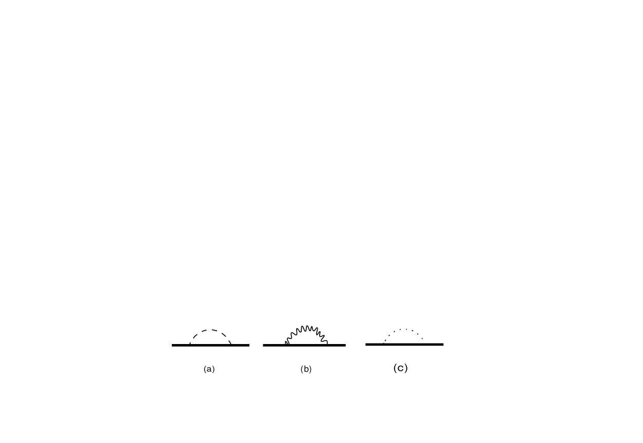
Figure 4: Self-energy diagrams for nucleon

Finally, we calculate nucleon self-energy diagrams. The pion contribution is given by

$$[\Sigma_{\pi}(\not\!p)]_{4c}=-(\frac{\lambda}{f_{\pi}})^{2}\frac{1}{16\pi^{2}}\frac{3}{4}[\frac{1}{2}(p^{2}-m^{2})\not\!p-m^{2}(\not\!p+m)]\frac{1}{\epsilon}~{}+~{}finite~{}terms$$ (30)

and that of $\sigma$-meson in Fig. 4 is given by

$$[\Sigma_{\sigma}(\not\!p)]_{4a}=-(\frac{\kappa}{f_{\sigma}})^{2}\frac{1}{16\pi^{2}}\frac{3}{4}[\frac{1}{2}(p^{2}-m^{2})\not\!p-m^{2}(\not\!p-m)]\frac{1}{\epsilon}~{}+~{}finite~{}terms.$$ (31)

In the Landau gauge, the $\rho$-meson contributions in Fig. 4 do not give wave function renormalization for nucleon fields. Then the corresponding renormalization constant $Z_{2}$ is given by

$$Z_{2} = 1+\frac{\partial\Sigma_{\pi}(\not\!p)}{\partial\not\!p}|_{\not p=m}+\frac{\partial\Sigma_{\sigma}(\not\!p)}{\partial\not\!p}|_{\not p=m}=1.$$ (32)

¿From eq.(29),

$$g_{\rho NN}^{B} = g_{\rho NN}\Lambda^{\epsilon}Z_{1}$$ (33)

$$= g_{\rho NN}\Lambda^{\epsilon}[1-(~{}\frac{3}{32\pi^{2}}gg_{\rho NN}+\frac{1}{8\pi^{2}}\frac{g_{\rho\pi\pi}}{g_{\rho NN}}(\frac{\lambda}{f_{\pi}})^{2}m^{2})\frac{1}{\epsilon}].$$

Then, the $\beta$-function for $g_{\rho NN}$ reads

$$\beta=-\frac{3gg_{\rho NN}^{2}}{16\pi^{2}}-\frac{1}{4\pi^{2}}g_{\rho\pi\pi}(\frac{\lambda}{f_{\pi}})^{2}m^{2}.$$ (34)

We can estimate the value of $\lambda$ by studying pion-nucleon interaction. In the chiral lagrangian, pion-nucleon interaction is described by $\frac{g_{A}}{f_{\pi}}\bar{\psi}\gamma_{5}\not\!\partial\pi\psi$[23] and that in our lagrangian is given by $\frac{\lambda}{f_{\pi}}\bar{\psi}\gamma_{5}\not\!\partial\pi\psi$. Then, we can conclude that $\lambda\simeq g_{A}$. So the value of $\lambda$ should be around $1$. After integrating the above renormalization group equation, we obtain the density dependent coupling constant($g_{\rho NN}$) through the arguments given in section 3. However the procedure may not be straightforward because there are many parameters (mass, coupling constants) which depend on the renormalization scale(density) in eq.(34), although we can conclude from the form of the $\beta$-function that $g_{\rho NN}$ drops as density increases.

Consider a simplest case, for example, without pion contribution (second term in eq.(34)) and with $\kappa=0$(where $g_{\rho NN}$ is equal to $g$). The $\beta$-function can be written as

$$\beta=-\frac{3g^{3}}{16\pi^{2}}.$$ (35)

Then, we can easily integrate out the renormalization group equation to obtain

$$g^{2}(\frac{\mu}{\mu_{0}})=\frac{g_{0}^{2}}{1+0.04g_{0}^{2}\ln\frac{\mu}{\mu_{0}}}$$ (36)

where $\mu_{0}$ is a reference chemical potential and $g_{0}^{2}=g^{2}(\frac{\mu}{\mu_{0}})|_{\mu=\mu_{o}}$. ¿From eq.(36), we can easily expect that $g^{2}(\mu)$(or $g^{2}_{\rho NN}$)drops slowly as density increases without pion contribution as depicted in Fig. 5. Our result is qualitatively agree with the result of ref.[24]. The density dependent coupling constant $g^{2}$ is used in ref.[25]. As we can see in eq.(34), the pion contributions play an important role in decreasing $g_{\rho NN}$ in dense nuclear matter. To see this more explicitly, let us solve eq.(34) in the case of $\kappa=0$ and $a=2$. In this case, the $\beta$-function is given by

$$\beta=-\frac{3g^{3}}{16\pi^{2}}-\frac{1}{4\pi^{2}}g\frac{\lambda^{2}}{f_{\pi}^{2}}m^{2}.$$ (37)

To solve eq.(37), we should also solve the renormalization group equations for $\frac{\lambda}{f_{\pi}}$ and $m$ and deal with the coupled renormalization group equations. But here we assume as a first approximation that the $\lambda$ and $a$ remains constant in dense matter and take $\lambda=1$. In ref.[17], it is shown that the parameter $a$ does not change very much against temperature. We also assume the relation, $\frac{m}{f_{\pi}}\simeq\frac{m^{*}}{f_{\pi}^{*}}\simeq 10$, to parameterize the density dependence of the $\frac{m}{f_{\pi}}$ economically . With these assumptions, we get the solution of eq.(37),

$$g^{2}(\frac{\mu}{\mu_{0}})=\frac{2.8g_{0}^{2}}{-0.02g_{0}^{2}+(2.8+0.02g_{0}^{2})(\frac{\mu}{\mu_{0}})^{5.6}}.$$ (38)

The results are depicted in Fig. 5 where we take $\mu_{0}=m$ for numerical purpose. If we make use of a simple relation, $\rho=\frac{2}{3\pi^{2}}(\mu^{2}-m^{2})^{3/2}$, we find that $\mu=\mu_{0}=m$ corresponds to $\rho=0$ and $\frac{\mu}{m}\simeq 1.14$ for $\rho=\rho_{0}(normal~{}nuclear~{}matter~{}density)$. Of course, the simple relation is no longer valid at high density. As it is mentioned, without the pion contribution, the $g_{\rho NN}$ drops slowly with density(solid line). If we include the pion contribution, we can see that the $g_{\rho NN}$ drops much faster with density(long-dashed line) in Fig. 5.

Let’s consider the renormalization of $\rho$-meson mass. The $\rho$-meson loop in Fig. 3 gives

$$[\Pi_{\mu\nu}]_{3e}=\frac{g^{2}}{16\pi^{2}}m_{\rho}^{2}6g^{\mu\nu}\frac{1}{\epsilon}$$ (39)

and $\rho$-meson tadpole in Fig. 3 gives

$$[\Pi_{\mu\nu}]_{3f}=-\frac{g^{2}}{16\pi^{2}}m_{\rho}^{2}\frac{9}{2}g^{\mu\nu}\frac{1}{\epsilon}$$ (40)

The corresponding renormalization constant $Z_{m_{\rho}}$ , which is defined as $m_{\rho}^{B}=Z_{m_{\rho}}m_{\rho}^{R}$, is given by

$$Z_{m_{\rho}}=1-\frac{3}{4}\frac{g^{2}}{(4\pi)^{2}}\frac{1}{\epsilon}.$$ (41)

Then, $\gamma_{m_{\rho}}$ is calculated to be

$$\gamma_{m_{\rho}}=\Lambda\frac{\partial}{\partial\Lambda}\ln Z_{m_{\rho}}=\frac{3}{2}\frac{g^{2}}{(4\pi)^{2}}.$$ (42)

We can obtain density dependent $\rho$-meson mass through renormalization group argument discussed in the section 3,

$$\mu\frac{d}{d\mu}m_{\rho}(\mu) = -(1+\frac{1}{2}\frac{3g^{2}}{(4\pi)^{2}})m_{\rho}(\mu)$$ (43)

$$\sim -1.37m_{\rho}(\mu)$$ (44)

for $a=2$. Neglecting the density dependence of the gauge coupling constant $g$, we get

$$m_{\rho}(\mu)=(\frac{\mu_{0}}{\mu})^{1.37}m_{\rho}(\mu_{0}),$$ (45)

which shows that the $\rho$-meson mass should drop as density increases as well as $\rho$-nucleon coupling constant in the low energy limit.

Let’s consider the effects of vector meson-nucleon tensor coupling. The interaction lagrangian is given by

$$L_{VN}=\frac{g\kappa_{\rho}}{2m}\bar{\Psi}(x)\sigma_{\mu\nu}\partial^{\mu}V^{\nu}\Psi(x)$$ (46)

where $\kappa_{\rho}\simeq 6$. We expect that the contributions from the tensor coupling may change the density dependence of $g_{\rho NN}$ substantially because of its anomalously large coupling constant($g\kappa_{\rho}\sim 36$).

The modification due to tensor coupling in the Fig. 2(a) is given by

$$[ig_{\rho NN}\Lambda_{\mu}^{a}]_{2a}=i\frac{1}{4}g_{\rho NN}T^{a}[\frac{3g^{2}\kappa_{\rho}^{2}}{128\pi^{2}}\frac{m_{\rho}^{2}}{m^{2}}-\frac{3gg_{\rho NN}\kappa_{\rho}}{32\pi^{2}}]\frac{1}{\epsilon}$$ (47)

and that in Fig. 2(b) is given by

$$[ig_{\rho NN}\Lambda_{\mu}^{a}]_{2b}=\frac{i}{16\pi^{2}}gT^{a}[\frac{g^{2}\kappa_{\rho}^{2}}{8m^{2}}(10m^{2}+6m_{\rho}^{2})+3gg_{\rho NN}\kappa_{\rho}]\frac{1}{\epsilon}$$ (48)

¿From these results and eq.(29), we find

$$Z_{1}=1 - [\frac{3}{32\pi^{2}}gg_{\rho NN}+\frac{1}{8\pi^{2}}\frac{g_{\rho\pi\pi}}{g_{\rho NN}}(\frac{\lambda}{f_{\pi}})^{2}m^{2}$$ (49)

$$+\frac{1}{4}(\frac{3g^{2}\kappa_{\rho}^{2}}{128\pi^{2}}\frac{m_{\rho}^{2}}{m^{2}}-\frac{3gg_{\rho NN}\kappa_{\rho}}{32\pi^{2}})$$

$$+\frac{1}{16\pi^{2}}\frac{g}{g_{\rho NN}}(\frac{g^{2}\kappa_{\rho}^{2}}{8m^{2}}(10m^{2}+6m_{\rho}^{2})+3gg_{\rho NN}\kappa_{\rho})]\frac{1}{\epsilon}.$$

Figure 5: The density(chemical potential) dependence of $g_{\rho NN}^{2}$. Here we take $\mu_{0}=m$. The solid line is for eq.(36) and the long-dashed one is for eq.(38). The short-dahsed line represents eq.(54).

Since the vector meson-nucleon tensor coupling is proportional to the momentum of $\rho$-meson, vector meson-nucleon tensor coupling does not play any role in the Fig. 3(a) in the low energy limit.

Consider the nucleon self-energy. As shown in the section 4.1, there are no wave function renormalizations for nucleon field. But with vector meson-nucleon tensor coupling, the Fig. 4(b) gives the wave function renormalization for nucleon field. The value of the Fig. 4(b) gets the following additional contributions from the tensor coupling,

$$[\Sigma_{\rho}^{VN}(\not p)]_{4b} = -\frac{3}{64\pi^{2}}[~{}\frac{g^{2}\kappa_{\rho}^{2}}{16m^{2}}(4p^{2}\not\!p-12m^{2}\not\!p-6m_{\rho}^{2}\not\!p-12m^{2}-12mm_{\rho}^{2})$$ (50)

$$-\frac{gg_{\rho NN}\kappa_{\rho}}{4m}(-6p^{2}+6m\not\!p+12m^{2}+12m_{\rho}^{2})~{}]\frac{1}{\epsilon}.$$

¿From this we get

$$Z_{2} = 1+\frac{\partial\Sigma_{\rho}^{VN}}{\partial\not\!p}|_{\not p=m}$$ (51)

$$= 1+\frac{3}{64\pi^{2}}[\frac{3g^{2}\kappa_{\rho}^{2}}{8}\frac{m_{\rho}^{2}}{m^{2}}-\frac{3}{2}gg_{\rho NN}\kappa_{\rho}]\frac{1}{\epsilon}.$$

As a first approximation, assuming that renormalization scale(density) dependence of $\kappa_{\rho}$ can be negligible, we get the modified $\beta$-function for $g_{\rho NN}$

$$\beta=-2c_{1}gg_{\rho NN}^{2}-c_{2}g^{2}g_{\rho NN}-2c_{3}g_{\rho\pi\pi}(\frac{\lambda}{f_{\pi}})^{2}-c_{2}g^{2}g_{\rho NN}-2c_{4}g^{3}$$ (52)

where $c_{i}$ are defined by

$$c_{1} = \frac{3}{32\pi^{2}}-\frac{1}{4}\frac{3\kappa_{\rho}}{32\pi^{2}}-\frac{3}{64\pi^{2}}\frac{3}{2}\kappa_{\rho},$$

$$c_{2} = \frac{1}{4}\frac{3\kappa_{\rho}^{2}}{128\pi^{2}}\frac{m_{\rho}^{2}}{m^{2}}+\frac{3\kappa_{\rho}}{16\pi^{2}}+\frac{3\kappa_{\rho}^{2}}{64\pi^{2}}\frac{3}{8}\frac{m_{\rho}^{2}}{m^{2}},$$

$$c_{3} = \frac{1}{8\pi^{2}}\frac{m^{2}}{f_{\pi}^{2}},$$

$$c_{4} = \frac{1}{16\pi^{2}}\frac{\kappa_{\rho}^{2}}{8}(10+6\frac{m_{\rho}^{2}}{m^{2}}).$$ (53)

The renormalization group equation eq.(52) can be solved with the $\kappa_{\rho}=6$, $\kappa=0$ and $a=2$ which are assumed to be independent of density. The result is given by

$$g^{2}(\frac{\mu}{\mu_{0}})=\frac{2.8g_{0}^{2}}{-1.04g_{0}^{2}+(2.8+1.04g_{0}^{2})(\frac{\mu}{\mu_{0}})^{5.6}}.$$ (54)

In Fig. 5, we can see that $g_{\rho NN}^{2}(\mu)$ drops much faster with the effects of tensor coupling than that without the effects of tensor coupling. So we conclude that the vector meson-nucleon tensor coupling as well as pions play an important role in decreasing the $g_{\rho NN}$ with density.

Figure 6: In-medium $\rho$-meson mass. Solid line represent the in-medium $\rho$-meson mass with density dependent coupling $g^{2}(\mu)$ and dashed lines represent the case of density independent coupling $g^{2}$.

5 Summary and Discussion

To study the properties of $\rho$-meson at finite density, we construct the effective lagrangian in which $\rho$-meson is identified as a dynamical gauge boson of hidden local symmetry. We have calculated the $\beta$-function for $\rho$-nucleon-nucleon coupling constant ($g_{\rho NN}$) and $\gamma$-function for $\rho$-meson mass ($\gamma_{m_{\rho}}$) at one loop approximation in the low energy limit.

Figure 7: The vertical axis denotes the ratio of in-medium $m_{\rho}^{2}$ to in-medium $2g^{2}$.

It is shown that these $\beta$-function and $\gamma$-function calculated in free space can be also used as $\beta$-function and $\gamma$-function in hadronic medium after changing the renormalization scale by the chemical potential as far as the thermodynamical potential is concerned. We also explicitly demonstrate that the $\rho$-meson mass and coupling constant for $\rho$-nucleon-nucleon vertex drop as density increases. Especially, we show that the pions and vector meson-nucleon tensor coupling give a dominant contribution to the $\beta$-function for $g_{\rho NN}$ and find that $g_{\rho NN}$ drops significantly even in normal nuclear matter density$(\rho_{0})$. So the density dependence of the coupling constants can affect the density dependence of $\rho$-meson mass substantially even in normal nuclear matter density because the $\rho$-meson self energy is a function of the coupling constants. For example, we solve eq.(43) with density dependent coupling constant($g^{2}(\mu)$) given in eq.(54). In Fig. 6, we depict in-medium $\rho$-meson mass with density independent coupling constant(dashed line) and the one with density dependent coupling constant(solid line). Although $g_{\rho NN}$ drops significantly even in normal nuclear matter density, the effects on in-medium $\rho$-meson mass is not so significant. This is because the coefficient ($\frac{1}{2}\frac{3}{(4\pi)^{2}}\sim 0.01$) of $g^{2}(\mu)$ in eq.(43) is much smaller than $1$ and so the change of $g^{2}(\mu)$ cannot modify the in-medium $\rho$-meson mass drastically.

Now we check whether the Kawarabayashi-Suzuki-Riazuddin-Fayyauddin (KSRF) relation holds in medium or not. At zero-temperature and zero-density the KSRF relation(for $\rho$-meson) is

$$m_{\rho}^{2}=2g_{\rho\pi\pi}^{2}f_{\pi}^{2}.$$ (55)

It is easy to see that $g_{\rho NN}=g=g_{\rho\pi\pi}$ when $\kappa\rightarrow 0$ and $a=2$ from eq.(7). To check whether the KSRF relation holds in medium or not, we plot the quantity $m_{\rho}^{2}(\mu)/(2g^{2}(\mu))$ which will be equal to $f_{\pi}^{2}(\mu)$ if the KSRF relation holds in medium. In Fig. 7, we see that $f_{\pi}^{2}(\mu)$ increases with density. But the $f_{\pi}^{2}(\mu)$ should decrease in medium[5][6][17]. Therefore, it seems that the KSRF relation does not hold in medium in our calculations.

In this work, we use several assumptions which are physically relevant for our analysis to solve the renormalization group equations. For the complete analysis, one may calculate, for example, all the $\beta$-function and $\gamma$-functions and solve coupled renormalization group equation as discussed in section 4. However we do not expect any substantial change in our conclusion. It will be interesting to study the effects of resonances[28] and to see how the resonances affect our results.

Finally, we discuss whether the non-renormalizability of our effective chiral lagrangian spoils the renormalization group arguments in section 3 or not. As it is well known, we can get rid of all the infinites in a non-renormalizable theory by including infinite number of counter terms allowed by symmetry [29]. Calculating the thermodynamic potential(pressure) with a diagram which involves a vertex from a non-renormalizable interaction, we may get a coefficient which depends both on the cut-off scale and on the chemical potential. As in Refs.[13][14], we do renormalizations before we do the four momentum integrations which introduce density effects to our thermodynamic potential or pressure. So it is impossible to get density or chemical potential($\mu$) dependent coefficients during renormalization. It is shown in the lectures[29] that in a mass-independent renormalization scheme, loop integrals do not have a power law dependence on any big scale such as cutoff. In the case of a mass-independent renormalization scheme, cutoff or renormalizaton scale only appears in logarithms. Since we have used mass-independent renormalization scheme in this paper, we don’t have any coeffient depending on some power of cutoff or renormalization scale during renormalization. So we don’t have a coefficient which depends both on the cut-off scale and on the chemical potential except logarithmic dependence. In Appendix, it is shown that this logarithmic dependence plays a very important role in our renormalization group analysis and therefore the non-renormalizability of our effective chiral lagrangian might not be crucial for the renormalization group arguments in section 3.

Appendix

In this Appendix, we present a simple model calculation to show how to calculate thermodynamic potential (pressure) and to see how the renormalization group equation works which we set up with some dimensional coupling constants such as $\frac{\lambda}{f_{\pi}}$. The lagrangian we are considering is given by

$${\it L}=\frac{1}{2}\partial_{\mu}\pi\partial^{\mu}\pi+\bar{\Psi}(x)i\gamma^{\mu}\partial_{\mu}\Psi(x)-m\bar{\Psi}(x)\Psi(x)+\frac{\lambda}{f_{\pi}}\bar{\Psi}(x)\gamma_{5}\gamma^{\mu}\partial_{\mu}\pi\Psi(x).$$ (A.2)

Figure 8: Self energy diagram for pion with counter term. Dotted line is for pion and solid line represents fermion.

Since here we are not interested in the thermodynamic potential (pressure) itself, we will consider only one type of graph and keep the terms which are essential in our renormalization group analysis. It can be easily seen in the QED example in section 3 that only the terms containing $\ln(\frac{\mu^{2}}{\Lambda^{2}})$ contribute to lowest order $\beta$-function. We also take the limit $\mu>>m$[13][14].

Now consider Fig. 8 (a) which is calculated to be

$$i\Pi(k^{2})=\frac{(mf_{\lambda})^{2}}{2\pi^{2}}k^{2}i[\frac{1}{\epsilon}-\ln{\frac{k^{2}}{\Lambda^{2}}}]$$ (A.3)

where $f_{\lambda}\equiv\frac{\lambda}{f_{\pi}}$ and $\Lambda$ is a renormalization scale. Introducing counter term, Fig. 8 (b), we obtain the pion wavefunction renormalization constant $Z_{\pi}$. Then, we can define

$$f_{\lambda}^{B}=f_{\lambda}Z_{\pi}^{-1/2}\Lambda^{\epsilon}$$ (A.4)

and we get the $\beta$-function for $f_{\lambda}$,

$$\beta_{\lambda}=\frac{(mf_{\lambda})^{2}}{2\pi^{2}}f_{\lambda}.$$ (A.5)

If our renormalization group anlysis is correct, the $\beta$-function eq.(A.5) must have something to do with a $\beta$-function defined in medium. To see this, we calculate the thermodynmic potential(or pressure) from Fig. 9 and Fig. 10.

Figure 9: $2nd$ order contribution to the thermodynamic potential. Here solid lines with $/$ denote the thermal(density) part of the fermion propagator[30].

In Fig. 10, we schematically draw how to renormalize the thermodynamic potential (pressure), for rigorous discussion see [13][14]. The thermodynamic potential (pressure) from Fig. 9 and Fig. 10 is given by

$$\Omega_{R}=\frac{(mf_{\lambda})^{2}}{16\pi^{4}}\mu^{4}+\frac{(mf_{\lambda})^{4}}{32\pi^{6}}\mu^{4}\ln\frac{\mu^{2}}{\Lambda^{2}}+...$$ (A.6)

where the $...$ represents the terms which are not important when we discuss the renormalization group analysis. This is obvious when we take a look at QED $\beta$-function discussed in section 3.

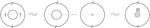
Figure 10: $4th$ order contribution to the thermodynamic potential. The brackets, $[$ $]$ indicate that we renormalize the enclosed diagram (pion self-energy) and $\Pi$ represents the finite part of the pion self-energy.

Now we construct renormalization equation following the procedure in section 3. Note that here we renormalize pion wavefunction only and therefore $f_{\lambda}$. Then the renormalization group equation for the thermodynamic potential, in this simple case, is given by

$$[\Lambda\frac{\partial}{\partial\Lambda}+\beta_{f_{\lambda}^{R}}(mf_{\lambda}^{R})\frac{\partial}{\partial f_{\lambda}^{R}}]\Omega_{R}(mf_{\lambda}^{R},\mu,\Lambda)=0$$ (A.7)

where we use $mf_{\lambda}^{R}$ instead of $f_{\lambda}^{R}$ because the coupling $f_{\lambda}^{R}$ carries a derivative(mass parameter) which is $m$ in our one loop calculations and the subscript $R$ denotes the renormalized parameters. The identity based on dimensional analysis is found to be

$$[\Lambda\frac{\partial}{\partial\Lambda}+\mu\frac{\partial}{\partial\mu}-4]\Omega_{R}(mf_{\lambda}^{R},\mu,\Lambda)=0.$$ (A.8)

From eq.(A.7) and eq.(A.8), we can write the following renormalization group equation

$$[\mu\frac{\partial}{\partial\mu}-\beta_{f_{\lambda}}(mf_{\lambda}^{R})\frac{\partial}{\partial f_{\lambda}^{R}}-4]\Omega_{R}(mf_{\lambda}^{R},\mu,\Lambda)=0.$$ (A.9)

The general solution is given by

$$\Omega_{R}(mf_{\lambda}^{R},\mu,\Lambda)=\mu^{4}{\bar{\Omega}}_{R}(mf_{\lambda}(\mu),\mu,\Lambda)$$ (A.10)

with a density dependent(effective or running) coupling constants defined by

$$\mu\frac{d}{d\mu}f_{\lambda}(\mu) = \beta_{\lambda}(mf_{\lambda}(\mu)).$$ (A.11)

Using the explicit form of the thermodynamic potential of eq. (A.6), we can show explicitly that the renormalization group equation, eq.(A.9), can be satisfied by identifyng $\beta_{\lambda}$ in eq. (A.11) with the one in eq.(A.5) to order of $m^{4}f_{\lambda}^{4}$,

$$[\mu\frac{\partial}{\partial\mu}-\frac{m^{2}f_{\lambda}^{2}(\mu)}{2\pi^{2}}f_{\lambda}(\mu)\frac{\partial}{\partial f_{\lambda}}-4]$$

$$\cdot(\frac{m^{2}f_{\lambda}^{2}(\mu)}{16\pi^{4}}\mu^{4}+\frac{m^{4}f_{\lambda}^{4}(\mu)}{32\pi^{6}}\mu^{4}\ln\frac{\mu^{2}}{\Lambda^{2}}+...)=0.$$ (A.12)

References

[1] G.E. Brown, G.Q. Li, R. Rapp, M. Rho
and J. Wambach, Acta. Phys. Pol. B29, 2309 (1998);
Y. Kim, R. Rapp, G.E. Brown and Mannque Rho, “A Schematic Model for
Density Dependent Vector Meson Masses,” nucl-th/9902009
[2] B. Friman, in Proceedings of the APCTP Workshop on
’Hadron Properties in Medium’, Seoul, Korea, Oct. 27-31, 1997, to be
published.
[3] F. Klingl, N.Kaiser and W. Weise,
Nucl. Phys. A 624, 527 (1997)
[4] G. Agakichiev et al., Phys. Rev. Lett. 75, 1272 (1995)
[5] G.E. Brown and M. Rho, Phys. Rev. Lett. 66, 2720 (1991)
[6]Y. Kim, H. K. Lee and M. Rho, Phys. Rev. C52, R1184 (1995);
Y. Kim and H. K. Lee, Phys. Rev. C55, 3100 (1997)
[7] A. K. D. Mazumder, B. D. Roy, A. Kundu and T. De,
Phys. Rev. C53, 790 (1996)
[8] R. Rapp, G. Chanfray and J. Wambach,
Nucl. Phys. A 617, 472 (1997)
[9] M. Bando, T. Kugo and K. Yamawaki, Phys. Rep. 164, 217
(1988) ; M. Bando et al., Phys. Rev. Lett. 54, 1215 (1985)
[10] J. I. Kapusta, Nucl. Phys. B148, 461 (1979)
[11] M. Matsumoto, Y. Nakano and H. Umezawa,
Phys. Rev. D29, 1116(1984)
[12] J.C. Collins and M.J. Perry,
Phys. Rev. Lett 34, 1353 (1975)
[14] B.A. Freedman and L. D. McLerran, Phys. Rev. D16,
1147 (1977)
[15] B.A. Freedman and L. D. McLerran, Phys. Rev. D16,
1169 (1977)
[16] S. Furui, R. Kobayashi and M. Nakagawa
Nuovo Cimento 108A, 241 (1995)
[17] M. Harada and A. Shibata, Phys. Rev. D55, 6716 (1997)
[18] G.E. Brown, E. Osnes and M. Rho, Phys. Lett. 163, 41 (1985)
[19] R. Machleidt, K. Holinde and C. Elster, Phys. Rep. 149,
1 (1987)
[20]M. Harada and K. Yamawaki, Phys. Lett. B297, 151(1992)
[21]J.-P. Blaizot, J. Korean Phys. Soc. 25, S65 (1992)
[22]Y. Ericson and W. Weise, Pions and Nuclei (Oxford
Science Publications, 1988).
[23] J. Gasser, M.E. Sainio and A. Svarc, Nucl. Phys.
B307, 779 (1988)
[24] M. Rho, Phys. Rept. 240, 1 (1994)
[25] C. Song, G.E. Brown D. -P. Min and M. Rho,
Phys. Rev. C56, 2244 (1997)
[26] M. Rho, Phys. Rev. Lett. 54, 767 (1985)
[27] M. Quiros, “Constraints on the higgs boson properties
from the effective potential,” hep-ph/9703412
[28] B. Friman and H.J. Pirner, Nucl. Phys.
A 617, 496 (1997); W. Peters, M. Post, H. Lenske, S. Leupold
and U. Mosel, Nucl. Phys. A 632, 109 (1998)
[29]D. B. Kaplan, “Effective Field Theories,” nucl-th/9506035;
A. V. Manohar, “Effective Field Theories,” hep-ph/9606222;
A. Pich, “Effective Field Theory,” hep-ph/9806303
[30]N.P. Landsman and C.G. van Weert, Phys. Rept. 145, 141 (1987)