Abstract

We analyze the evolution equation describing all multiple hard pomeron exchanges in a hadronic or nuclear structure functions that was proposed earlier in [1]. We construct a perturbation series providing us with an exact solution to the equation outside of the saturation region. The series demonstrates how at moderately high energies the corrections to the single BFKL pomeron exchange contribution which are due to the multiple pomeron exchanges start unitarizing total deep inelastic scattering cross section. We show that as energy increases the scattering cross section of the quark–antiquark pair of a fixed transverse separation on a hadron or nucleus given by the solution of our equation inside of the saturation region unitarizes and becomes independent of energy. The corresponding $F_{2}$ structure function also unitarizes and becomes linearly proportional to $\ln s$. We also discuss possible applications of the developed technique to diffraction.

I Introduction

The Balitsky, Fadin, Kuraev and Lipatov (BFKL) [2, 3] equation resums all leading logarithms of Bjorken $x$ for hadronic cross sections and structure functions. The solution of the BFKL equation grows like a power of center of mass energy $s$, therefore violating the unitarity bound at very high energies [4, 5]. This is one of the major problems of small $x$ physics, since the Froissart bound [4, 5] states that the total cross section should not raise faster than $\ln^{2}s$ at asymptotically high energies. There is a general belief that the unitarity problem could be cured by resumming all multiple BFKL pomeron exchanges in the total cross section, or, equivalently, in the structure function.

As was argued by Mueller in [6] multiple pomeron exchanges become important at the values of rapidity of the order of

$$Y_{U}\sim\frac{1}{\alpha_{P}-1}\,\ln\frac{1}{\alpha^{2}},$$ (1)

with $\alpha$ the strong coupling constant, which is assumed to be small, and $\alpha_{P}-1=\frac{4\alpha N_{c}}{\pi}\ln 2$. This result could be obtained if one notes that one pomeron contribution to the total cross section of, for instance, onium–onium scattering, is parametrically of the order of $\alpha^{2}\exp[(\alpha_{P}-1)Y]$ and the contribution of the double pomeron exchange is $\alpha^{4}\exp[2(\alpha_{P}-1)Y]$. Since multiple pomeron exchanges become important when the single and double pomeron exchange contributions become comparable, we recover Eq. (1) by just equating the two expressions.

After completion of the calculation of the next–to–leading order corrections to the kernel of the BFKL equation (NLO BFKL) by Fadin and Lipatov [7], and, independently, by Camici and Ciafaloni [8], it was shown in [9] that due to the running coupling effects these corrections become important at the rapidities of the order of

$$Y_{NLO}\sim\frac{1}{\alpha^{5/3}}.$$ (2)

One can see that $Y_{U}\ll Y_{NLO}$ for parametrically small $\alpha$. That implies that the center of mass energy at which the multiple pomeron exchanges become important is much smaller, and, therefore, is easier to achieve, than the energy at which NLO corrections start playing an important role. That is multiple pomeron exchanges are probably more relevant than NLO BFKL to the description of current experiments [10]. Also multiple pomeron exchanges are much more likely to unitarize the total hadronic cross section. In this paper we are going to propose a solution to the problem of resummation of multiple pomeron exchanges and show how the BFKL pomeron unitarizes.

FIG. 1.: An example of the pomeron “fan” diagram.

In the previous paper on the subject [1] we proposed an equation which resums all multiple BFKL pomeron [2, 3] exchanges in the nuclear structure function. In deriving the equation we used the techniques of Mueller’s dipole model [11, 12, 13, 14]. As was proven some time ago [11, 15] the dipole model can provide us with the equation which is exactly equivalent to the BFKL equation [2, 3]. In [1] it was shown that the dipole model methods, when applied to hadronic or nuclear structure functions, yield us with the equation which in the traditional Feynman diagram language resums the so–called pomeron “fan” diagrams in the leading logarithmic approximation, an example of which is depicted in Fig. 1 for the case of deep inelastic scattering.

To review the results of [1] let us consider a deep inelastic scattering (DIS) of a virtual photon on a hadron or a nucleus. An incoming photon splits into a quark–antiquark pair and then the $q{\overline{q}}$ pair rescatters on the target hadron. In the rest frame of the hadron all QCD evolution should be included in the wave function of the incoming photon. That way the incoming photon develops a cascade of gluons, which then scatter on the hadron at rest. In [1] this gluon cascade was taken in the leading longitudinal logarithmic ($\ln 1/x$) approximation and in the large $N_{c}$ limit. This is exactly the type of cascade described by Mueller’s dipole model [11, 12, 13, 14]. In the large $N_{c}$ limit the incoming gluon develops a system of color dipoles and each of them independently rescatters on the hadron (nucleus) [1]. The forward amplitude of the process is shown in Fig. 2. The double lines in Fig. 2 correspond to gluons in large $N_{c}$ approximation being represented as consisting of a quark and an antiquark of different colors. The color dipoles are formed by a quark from one gluon and an antiquark from another gluon. In Fig. 2 each dipole, that was developed through the QCD evolution, later interacts with the nucleus by a series of Glauber–type multiple rescatterings on the nucleons. The assumption about the type of interaction of the dipoles with the hadron or nucleus is not important for the evolution. It could also be just two gluon exchanges. The important assumption is that each dipole interacts with the target independently of the other dipoles, which is done in the spirit of the large $N_{c}$ limit.

For the case of a large nucleus independent dipole interactions with the target nucleus are enhanced by some factors of the atomic number $A$ of the nucleus compared to the case when several dipoles interact with the same nucleon [1]. This allowed us to assume that the dipoles interact with the nucleus independently. The summation of these contribution corresponds to summation of the pomeron “fan” diagrams of Fig. 1. However, in general there is another class of diagrams, which we will call pomeron loop diagrams. In a pomeron loop diagram a pomeron first splits into two pomerons, just like in the fan diagram, but then the two pomerons merge back into one pomeron. In other words the graphs containing pomerons not only splitting, but also merging together will be referred to as pomeron loop diagrams. In a large nucleus these pomeron loop diagrams could be considered small, since they would be suppressed by powers of $A$. This approximation strictly speaking is not valid for the calculation of a hadronic wave function. At very high energies it also becomes not very well justified even in the nuclear case for the following reason. The contribution of each additional pomeron in a fan diagram on a nucleus is parametrically of the order of $\alpha^{2}A^{1/3}e^{(\alpha_{P}-1)Y}$, which is large at the rapidities of the order of $Y_{U}$ given by Eq. (1). The contribution of an extra pomeron in a pomeron loop diagram is of the order of $\alpha^{2}e^{(\alpha_{P}-1)Y}$, which is not enhanced by powers of $A$ and is, therefore, suppressed in the nuclear case. However, one can easily see that at extremely high energies, when $\alpha^{2}e^{(\alpha_{P}-1)Y}$ becomes greater than or of the order of one, pomeron loop diagrams become important even for a nucleus, still being smaller than the fan diagrams.

FIG. 2.: Dipole evolution in the deep inelastic scattering process as pictured in Ref.[1]. The incoming virtual photon develops a system of color dipoles, each of which rescatters on the nucleus (only two are shown).

Resummation of pomeron loop diagrams in a dipole wave function seems to be a very hard technical problem, possibly involving NLO BFKL or, even, next-to-next-to-leading order BFKL kernel calculations [16]. Nevertheless, it is the author’s belief that these pomeron loop diagrams are not going to significantly change the high energy behavior of the structure functions. Still in the rigorous sense the results of this paper should be considered as resumming the fan diagrams only, which is strictly justified only for a large nucleus.

In [1], rewriting the $F_{2}$ structure function of the target as a convolution of the wave function of the $q\overline{q}$ fluctuations of a virtual photon with the propagator of the quark–antiquark pair through the nucleus, we obtained

$$F_{2}(x,Q^{2})=\frac{Q^{2}}{4\pi^{2}\alpha_{EM}}\int\frac{d^{2}{\bf x}_{01}dz}{2\pi}\,\Phi({\bf x}_{01},z)\ d^{2}b_{0}\ N({\bf x}_{01},{\bf b}_{0},Y),$$ (3)

where the photon’s wave function

$$\Phi({\bf x}_{01},z)=\Phi_{T}({\bf x}_{01},z)+\Phi_{L}({\bf x}_{01},z)$$ (4)

consists of transverse

$$\Phi_{T}({\bf x}_{01},z)=\frac{2N_{c}\alpha_{EM}}{\pi}a^{2}\ K_{1}^{2}(x_{01}a)\ [z^{2}+(1-z)^{2}]$$ (6)

and longitudinal

$$\Phi_{L}({\bf x}_{01},z)=\frac{2N_{c}\alpha_{EM}}{\pi}\ 4Q^{2}z^{2}(1-z)^{2}\ K_{0}^{2}(x_{01}a)$$ (7)

contributions, with $a^{2}=Q^{2}z(1-z)$, and we assumed that quarks are massless and have only one flavor and unit electric charge. As always $Q^{2}$ is the virtuality of the photon and $x$ is the Bjorken $x$-variable. $z$ is the fraction of the photons light cone momentum carried by the quark, ${\bf x}_{01}={\bf x}_{1}-{\bf x}_{0}$ is the transverse separation of the quark–antiquark pair, ${\bf b}_{0}$ is the impact parameter of the original pair and $Y\sim\ln(1/x)$ is the rapidity variable. $N({\bf x}_{01},{\bf b}_{0},Y)$ is the propagator of the quark–antiquark pair through the nucleus, or, more correctly, the forward scattering amplitude of the $q\overline{q}$ pair with the nucleus (hadron). It obeys the equation [1]

$$N({\bf x}_{01},{\bf b}_{0},Y)=-\gamma({\bf x}_{01},{\bf b}_{0})\,\exp\left[-\frac{4\alpha C_{F}}{\pi}\ln\left(\frac{x_{01}}{\rho}\right)Y\right]+\frac{\alpha C_{F}}{\pi^{2}}\int_{0}^{Y}dy\,\exp\left[-\frac{4\alpha C_{F}}{\pi}\ln\left(\frac{x_{01}}{\rho}\right)(Y-y)\right]$$

$$\times\int_{\rho}d^{2}x_{2}\frac{x_{01}^{2}}{x_{02}^{2}x_{12}^{2}}\,[2\,N({\bf x}_{02},{\bf b}_{0}+\frac{1}{2}{\bf x}_{12},y)-N({\bf x}_{02},{\bf b}_{0}+\frac{1}{2}{\bf x}_{12},y)\,N({\bf x}_{12},{\bf b}_{0}+\frac{1}{2}{\bf x}_{02},y)],$$ (8)

with $\gamma({\bf x}_{01},{\bf b}_{0})$ the propagator of a dipole of size ${\bf x}_{01}$ at the impact parameter ${\bf b}_{0}$ through the target nucleus or hadron, which was taken to be of Glauber form in [1]:

$$\gamma({\bf x}_{01},{\bf b}_{0})=\exp\left[-\frac{\alpha\pi^{2}}{2N_{c}S_{\perp}}{\bf x}_{01}^{2}AxG(x,1/{\bf x}_{01}^{2})\right]-1.$$ (9)

here $S_{\perp}$ is the transverse area of the hadron or nucleus, $A$ is the atomic number of the nucleus, and $xG$ is the gluon distribution of the nucleons in the nucleus, which was taken at the two gluon (lowest in $\alpha$) level [17]. Eq. (9) is written for a cylindrical hadron or nucleus. In the large $N_{c}$ limit $C_{F}\approx N_{c}/2$. In Eq. (8) $\rho$ is an ultraviolet regulator [1, 11].

Eq. (8) resums all multiple hard pomeron exchanges in the $F_{2}$ structure function. The linear in $N$ term on the right hand side of Eq. (8) corresponds to the usual BFKL evolution [11], whereas the quadratic term in $N$ is in a certain way responsible for triple pomeron vertices. This quadratic term on the right hand side of Eq. (8) introduces some damping effects, which at the end unitarize the growth of the BFKL pomeron. We note that an equation similar to (8) was suggested by Gribov, Levin and Ryskin (GLR) in momentum space representation in [18] and was subsequently studied by Bartels and Levin in [19]. However, usually by the GLR equation one implies an equation summing all fan diagrams in the double leading logarithmic approximation. Eq. (8) resums all the fan diagram in the leading longitudinal logarithmic approximation. In the double logarithmic limit (large $Q^{2}$) Eq. (8) reduces to the GLR equation. We also note that an equation very similar to Eq. (8) has been proposed by Balitsky in [20] to be used in describing the wavefunctions of each of the quarkonia in onium–onium scattering, similarly to [12, 21]. A renormalization group techniques based on McLerran–Venugopalan [22] model have been developed by Jalilian-Marian, Kovner, Leonidov, and Weigert [23] leading to an equation which is also supposed to resum multiple hard pomeron exchanges [23]. Unfortunately the resulting equation [23] differs from our Eq. (8). An equation summing all multiple pomeron diagrams in the double logarithmic limit has been proposed by Ayala, Gay Ducati and Levin [24], which is also different from the appropriate limit of our Eq. (8).

In this paper we are going to analyze Eq. (8). In Sect. II we will find a solution of Eq. (8) in the form of a series in Eq. (34) which will be constructed by solving Eq. (8) perturbatively in the momentum space. The details of transforming Eq. (8) into momentum space will be given in the Appendix A with the result given by Eq. (14). The terms of the series will correspond to multiple pomeron exchange contributions. Partial sums of the series will be plotted in Fig. 3, which shows how multiple pomeron exchanges unitarize the amplitude. We will argue that the kinematic region for which the series is convergent corresponds to the case when the DIS cross sections and structure functions have not reached saturation. In a certain sense we will define the saturation region as the kinematic regime where the series ceases to converge. By resumming the terms of the series corresponding to exchanges of large numbers of pomerons we construct a function which we can analytically continue outside the region of convergence of the series of Eq. (34). That would provide us with the ansatz for the solution of Eq. (14) outside of the saturation region [see Eq. (55)]. We will prove that this ansatz actually is the only possible energy independent solution of Eq. (14).

To transform our results into coordinate space on would have to separate the momentum integration in two regions, one of them being above and the other one being below the saturation scale. Since we will find only the asymptotic solution inside the saturation region our results may not be very precise in determining the coordinate space amplitude. A numerical solution of Eq. (8) would probably allow one to achieve better precision. Nevertheless for asymptotically high energies we can transform the amplitude into coordinate space obtaining Eq. (56). Thus we will show that multiple pomeron exchanges unitarize the forward amplitude, making it independent of energy at high energies, which is shown in Fig. 4.

In Sect. III we will analyze the high energy asymptotics of the $F_{2}$ structure function. We will show that, contrary to some expectations, $F_{2}$ structure function does not become independent of energy at high energies. It becomes linearly proportional to $\ln s$, still satisfying the Froissart bound [see Eq. (64)].

In Sect. IV we will discuss how in the framework of the dipole model one can describe diffractive scattering by including the multiple pomeron evolution in rapidity of Eq. (8) in the quasi–elastic structure functions considered in [25]. We will derive an expression for the quasi–elastic structure function $F_{2}^{D}$ (70) and discuss its asymptotics (72). Finally, we will conclude in Sect. V by summarizing our results and discussing the possible implications of the developed techniques on different issues of small-$x$ physics.

II Perturbative solution of the evolution equation

We start by considering a DIS on a large cylindrical nucleus. This assumption about the size and geometry of the nucleus is being done for simplicity of calculations and our results could be easily generalized to a large nucleus of any shape. If the nucleus is sufficiently large we can assume that the forward amplitude of the scattering of the original quark–antiquark pair on the nucleus, $N({\bf x}_{01},{\bf b}_{0},Y)$, is a slowly varying function of the impact parameter of the virtual photon ${\bf b}_{0}$. This is equivalent to assuming that the transverse extent of the dipole wave function is much smaller than the size of the nucleus, and that the impact parameter between the virtual photon and the nucleus is smaller than the radius of the nucleus $R$. We note that in order to construct $N({\bf x}_{01},{\bf b}_{0},Y)$ in [1] we integrated over the impact parameters ${\bf b}_{i}$’s of the nucleons with which each of the pomerons in Fig. 1 interacted. That way ${\bf b}_{0}$ does not have a meaning of the impact parameter of a pomeron exchange anymore and ${\bf b}_{0}$ dependence in $N({\bf x}_{01},{\bf b}_{0},Y)$ becomes purely “geometrical” . In a more formal language we assume that $x_{\perp}\ll R$, where $x_{\perp}$ is the typical transverse size of the dipole wave function, and $b_{0}<R$ ($b_{0}$ is zero at the center of the nucleus). If these conditions are satisfied we may neglect ${\bf x}_{12}$ and ${\bf x}_{02}$ compared to ${\bf b}_{0}$ on the right hand side of Eq. (8), which means that the changes in $N({\bf x}_{01},{\bf b}_{0},Y)$ when ${\bf b}_{0}$ is varied by ${\bf x}_{\perp}$ are negligibly small. Thus suppressing the ${\bf b}_{0}$ dependence we write $N({\bf x}_{01},Y)$ instead of $N({\bf x}_{01},{\bf b}_{0},Y)$ in Eq.(8). Then differentiating Eq. (8) with respect to $Y$ we can rewrite it as

$$\frac{\partial N({\bf x}_{01},Y)}{\partial Y}=\frac{2\alpha C_{F}}{\pi^{2}}\,\int_{\rho}d^{2}x_{2}\left[\frac{x^{2}_{01}}{x^{2}_{02}x^{2}_{12}}-2\pi\delta^{2}({\bf x}_{01}-{\bf x}_{02})\ln\left(\frac{x_{01}}{\rho}\right)\right]N({\bf x}_{02},Y)$$

$$-\frac{\alpha C_{F}}{\pi^{2}}\,\int d^{2}x_{2}\,\frac{x^{2}_{01}}{x^{2}_{02}x^{2}_{12}}\,N({\bf x}_{02},Y)\,N({\bf x}_{12},Y),$$ (10)

with $N({\bf x}_{01},0)=-\gamma({\bf x}_{01})$ as the initial condition, where we also suppressed (but did not neglect) the impact parameter dependence of $\gamma$. Now one can see that the evolution equation (10) itself in the large nucleus approximation does not impose any impact parameter ${\bf b}_{0}$ dependence. The latter is only included in the initial conditions given by $\gamma({\bf x}_{01},{\bf b}_{0})$. Since $\gamma$ is a slowly varying function of ${\bf b}_{0}$ (constant for a cylindrical nucleus) our assumption about the slow dependence of $N$ on ${\bf b}_{0}$ is self consistent. Physically this implies that before the collision, when the incoming virtual photon develops its dipole evolved wave function, it does not have any information about the nucleus. The information about the thickness of the nuclear medium as a function of the impact parameter comes through $\gamma$ when the dipoles interact with the nucleus.

Let us rewrite

$$N(x_{\perp},Y)=x_{\perp}^{2}\int\frac{d^{2}k}{2\pi}\,e^{i{\bf k}\cdot{\bf x}}\,{\tilde{N}}(k,Y)=x_{\perp}^{2}\int_{0}^{\infty}dk\,k\,J_{0}(kx_{\perp})\,{\tilde{N}}(k,Y).$$ (12)

We note that the inverse of this transformation is

$${\tilde{N}}(k,Y)=\int\frac{d^{2}x}{2\pi x_{\perp}^{2}}\,e^{-i{\bf k}\cdot{\bf x}}\,N(x_{\perp},Y)=\int_{0}^{\infty}\frac{dx_{\perp}}{x_{\perp}}\,J_{0}(kx_{\perp})\,N(x_{\perp},Y).$$ (13)

Since $N(x_{\perp},Y)$ does not depend on the direction of ${\bf x}_{\perp}$, ${\tilde{N}}(k,Y)$ does not depend on the direction of the relative transverse momentum of the $q\overline{q}$ pair ${\bf k}_{\perp}$. That allowed us to simplify the integrations in Eqs. (12) and (13). Now Eq. (10) becomes

$$\frac{\partial{\tilde{N}}(k,Y)}{\partial Y}=\frac{2\alpha N_{c}}{\pi}\,\chi\left(-\frac{\partial}{\partial\ln k}\right)\,{\tilde{N}}(k,Y)-\frac{\alpha N_{c}}{\pi}\,{\tilde{N}}^{2}(k,Y),$$ (14)

where

$$\chi(\lambda)=\psi(1)-\frac{1}{2}\psi\left(1-\frac{\lambda}{2}\right)-\frac{1}{2}\psi\left(\frac{\lambda}{2}\right)$$ (15)

is the eigenvalue of the BFKL kernel [2, 3, 11] with $\psi(\lambda)=\Gamma^{\prime}(\lambda)/\Gamma(\lambda)$. In Eq. (14) the function $\chi(\lambda)$ is taken as a differential operator with $\lambda=-\partial/\partial\ln k$ acting on ${\tilde{N}}(k,Y)$. We also put $N_{c}/2$ instead of $C_{F}$ everywhere in the spirit of the large $N_{c}$ approximation. The details of obtaining Eq. (14) from Eq. (10) are presented in the Appendix A. Eq. (14) shows explicitly that the first, linear, term on its right hand side gives the usual BFKL equation, whereas the quadratic term corresponds to the triple pomeron vertex, which unitarizes the growth of the BFKL pomeron.

One can easily prove that Eq. (14) has a unique solution satisfying given initial condition at $Y=0$. The strategy of the proof is conventional: assume that there are two different solutions of Eq. (14) satisfying given initial conditions. Then one can easily derive an equation for the function given by the difference of these solutions with the initial condition stating that the function is equal to zero when $Y=0$. After a little analysis of the resulting equation with that initial condition one could easily see that the difference between the two solutions of the original Eq. (14) is zero. That way one proves uniqueness of the solution of Eq. (14).

We want to find a solution of Eq. (14) satisfying the initial condition given by the BFKL pomeron contribution at relatively “small” rapidity $Y\sim 1/\alpha$. Unfortunately finding an exact analytical solution of Eq. (14) seems to be a very difficult task, partly because Eq. (14) is non–linear, partly because of a complicated structure of the BFKL kernel $\chi(\lambda)$. Instead we are going to construct a series resulting from the perturbative solution of Eq. (14), which, in the region where it is convergent, provides us with the exact solution of Eq. (14). As we will show below the region of convergence of that series corresponds to the regime when the DIS cross sections and structure functions are not saturated. In the saturation regime the series diverges, but allows us to construct an asymptotic solution by analytical continuation.

Let us start by assuming that at $Y\sim 1/\alpha$ the function $\tilde{N}$ is very small, $\tilde{N}\ll 1$. This allows us to neglect the quadratic term in Eq. (14), since it would be of higher order in $\tilde{N}$. Then Eq. (14) becomes

$$\frac{\partial{\tilde{N}}_{1}(k,Y)}{\partial Y}=\frac{2\alpha N_{c}}{\pi}\,\chi\left(-\frac{\partial}{\partial\ln k}\right)\,{\tilde{N}}_{1}(k,Y),$$ (16)

which corresponds to the usual BFKL equation [2, 3]. The solution of Eq. (16) is given by

$${\tilde{N}}_{1}(k,Y)=\exp\left[\frac{2\alpha N_{c}}{\pi}\,Y\,\chi\left(-\frac{\partial}{\partial\ln k}\right)\right]\,C(k),$$ (17)

with $C(k)$ being some unknown function of $k$, to be specified by initial conditions.

Rewrite $C(k)$ as a Mellin transformation

$$C(k)=\int\frac{d\lambda}{2\pi i}\left(\frac{k}{\Lambda}\right)^{\lambda}C_{\lambda},$$ (18)

where $\Lambda\sim\Lambda_{QCD}$ is some scale characterizing the nucleus or hadron. Here the integration in $\lambda$ runs parallel to the imaginary axis to the right of all the singularities of $C_{\lambda}$. Substituting Eq. (18) into Eq. (17) we obtain

$${\tilde{N}}_{1}(k,Y)=\int\frac{d\lambda}{2\pi i}\,\exp\left[\frac{2\alpha N_{c}}{\pi}\,Y\,\chi\left(-\lambda\right)\right]\left(\frac{k}{\Lambda}\right)^{\lambda}C_{\lambda}.$$ (19)

Assuming that the transverse momentum of the $q\overline{q}$ pair $k$ is not very large, such that $\ln(k/\Lambda)\ll\alpha YN_{c}$ and that $C_{\lambda}(Y)$ is a slowly varying function of $\lambda$ we come to the conclusion that the integral in Eq. (19) is dominated by the saddle point in the exponential in the vicinity of $\lambda=-1$ in $\chi(-\lambda)$. Expanding $\chi(-\lambda)\approx 2\ln 2+\frac{7}{4}\zeta(3)(\lambda+1)^{2}$, with $\zeta(z)$ the Riemann zeta function, we can perform a saddle point approximation in the integral of Eq. (19). The saddle point is given by

$$\lambda_{sp}=-1-a(k,Y),$$ (20)

where we have defined

$$a(k,Y)=\frac{\pi\ln(k/\Lambda)}{7\alpha N_{c}\zeta(3)Y},$$ (21)

which is small. The result of the integration yields

$${\tilde{N}}_{1}(k,Y)=C_{-1}\,\frac{\Lambda}{k}\,\frac{\exp[(\alpha_{P}-1)Y]}{\sqrt{14\alpha N_{c}\zeta(3)Y}}\exp\left(-\frac{\pi}{14\alpha N_{c}\zeta(3)Y}\ln^{2}\frac{k}{\Lambda}\right)\equiv P_{1}(k,Y),$$ (22)

a factor usually associated with the zero momentum transfer single hard pomeron exchange, which we denoted by $P_{1}$. $C_{-1}$ is determined from initial conditions. If the initial conditions are given by the two gluon exchange approximation, then $C_{-1}\sim\alpha^{2}$. That way, parametrically, when $Y\sim 1/\alpha$, the amplitude $\tilde{N}_{1}\sim\alpha^{2}\ll 1$, and our assumption of the smallness of $\tilde{N}$ at $Y\sim 1/\alpha$ is justified.

Eq. (22) provides us with the usual single BFKL pomeron solution. Now we are going to find corrections to this expression resulting from Eq. (14), which will form a series

$$\tilde{N}(k,Y)=\sum_{n=1}^{\infty}{\tilde{N}}_{n}(k,Y),$$ (23)

with ${\tilde{N}}_{n}$ being of the order of ${\tilde{N}}_{1}^{n}$. The first correction is ${\tilde{N}}_{2}$. Rewriting ${\tilde{N}}={\tilde{N}}_{1}+{\tilde{N}}_{2}$, substituting it back into Eq. (14), neglecting non–linear terms in ${\tilde{N}}_{2}$ and employing Eq. (16) we obtain

$$\frac{\partial{\tilde{N}}_{2}(k,Y)}{\partial Y}=\frac{2\alpha N_{c}}{\pi}\,\chi\left(-\frac{\partial}{\partial\ln k}\right)\,{\tilde{N}}_{2}(k,Y)-\frac{\alpha N_{c}}{\pi}\,{\tilde{N}}_{1}(k,Y)^{2},$$ (24)

where ${\tilde{N}}_{1}$ is given by Eq. (19). One can easily see that the solution of Eq. (24) with the initial condition that it disappears at small $Y$ is

$${\tilde{N}}_{2}(k,Y)=-\frac{\alpha N_{c}}{\pi}\int_{0}^{Y}dy\exp\left[\frac{2\alpha N_{c}}{\pi}\,(Y-y)\,\chi\left(-\frac{\partial}{\partial\ln k}\right)\right][{\tilde{N}}_{1}(k,y)^{2}].$$ (25)

Plugging ${\tilde{N}}_{1}$ of Eq. (19) into Eq. (25) and integrating over $y$ yields

$${\tilde{N}}_{2}(k,Y)=-\int\frac{d\lambda_{1}\,d\lambda_{2}}{(2\pi i)^{2}}\,C_{\lambda_{1}}\,C_{\lambda_{2}}\,\left(\frac{k}{\Lambda}\right)^{\lambda_{1}+\lambda_{2}}\,\frac{1}{2[\chi(-\lambda_{1})+\chi(-\lambda_{2})-\chi(-\lambda_{1}-\lambda_{2})]}$$

$$\times\left[\exp\left(2\,\frac{\alpha N_{c}}{\pi}\,Y\,[\chi(-\lambda_{1})+\chi(-\lambda_{2})]\right)-\exp\left(2\,\frac{\alpha N_{c}}{\pi}\,Y\,\chi(-\lambda_{1}-\lambda_{2})\right)\right].$$ (26)

Eq. (24) corresponds to putting one triple pomeron vertex (given by quadratic term in ${\tilde{N}}$) into the DIS diagram, so that ${\tilde{N}}_{2}$ consists of one pomeron splitting into two. The integration over $y$ in Eq. (25) corresponds to integration over all possible rapidity positions of the triple pomeron vertex between the incoming quark–antiquark pair and the target. Thus the first exponential term in the square brackets in Eq. (26) corresponds to the case when the pomeron splitting occurs very close (in rapidity) to the $q\overline{q}$ pair, so that most of the rapidity interval is covered by two pomeron contribution. The second exponential term in Eq. (26) corresponds to the situation when the splitting happens very close to the target, so that most of the interaction corresponds to the single pomeron exchange. Therefore the first exponential term in Eq. (26) corresponds to two pomeron contribution and the second term corresponds to the one pomeron contribution. Similar conclusions have been reached by Navelet and Peschanski in [21] when analyzing two pomeron contribution to onium–onium scattering in dipole model [12]. As we will see below the two pomeron contribution gives a term proportional to $\exp[2(\alpha_{P}-1)Y]$, while the one pomeron exchange is proportional to $\exp[(\alpha_{P}-1)Y]$. That way the two pomeron term dominates in ${\tilde{N}}_{2}$ and the single pomeron term could be safely neglected. One should also remember that ${\tilde{N}}_{2}$ is proportional to the square of $C_{\lambda}$, so that the single pomeron exchange term from ${\tilde{N}}_{2}$ represents just an order $\alpha^{2}$ (i.e., next-to-next-to-leading order) correction to ${\tilde{N}}_{1}$. Neglecting this contribution we rewrite Eq. (26) as

$${\tilde{N}}_{2}(k,Y)=-\int\frac{d\lambda_{1}\,d\lambda_{2}}{(2\pi i)^{2}}\,C_{\lambda_{1}}\,C_{\lambda_{2}}\,\left(\frac{k}{\Lambda}\right)^{\lambda_{1}+\lambda_{2}}\,\frac{1}{2[\chi(-\lambda_{1})+\chi(-\lambda_{2})-\chi(-\lambda_{1}-\lambda_{2})]}$$

$$\times\exp\left(2\,\frac{\alpha N_{c}}{\pi}\,Y\,[\chi(-\lambda_{1})+\chi(-\lambda_{2})]\right).$$ (27)

Here again we can perform the integration over $\lambda_{1}$ and $\lambda_{2}$ in the saddle point approximation. The saddle points of $\lambda_{1}$ and $\lambda_{2}$ integrations would have been independent if it were not for the $\chi(-\lambda_{1}-\lambda_{2})$ in the denominator. The problem is that $\chi(\lambda)$ has a pole at $\lambda=2$, and since the saddle points of $\lambda_{1}$ and $\lambda_{2}$ integrations are located in the vicinity of $-1$ [see Eq. (20)] this could influence the exact location of the saddle points of the integral. However, as one can see analyzing the saddle points of Eq. (27), if $\ln^{2}(k/\Lambda)>\alpha YN_{c}$ the effect of $\chi(-\lambda_{1}-\lambda_{2})$ could be safely neglected. This imposes an additional constraint on the possible values of transverse momentum $k$. Remember that in order to perform the saddle point integration in Eq. (19) we had to assume that $\ln(k/\Lambda)\ll\alpha YN_{c}$. These two conditions specify the range of $k$ in which our analysis is applicable. The condition $\ln^{2}(k/\Lambda)>\alpha YN_{c}$ is not very hard to satisfy, since, after all, the transverse momentum $k$ should be large enough for perturbative QCD to be applicable, i.e. , $\ln(k/\Lambda)\gg 1$. We will return to this question below.

Performing the saddle point integration in Eq. (27) in the spirit of the above discussion one obtains

$${\tilde{N}}_{2}(k,Y)=-\frac{a(k,Y)}{1+8\,a(k,Y)\,\ln 2}\,P_{1}(k,Y)^{2},$$ (28)

with $a(k,Y)$ defined in Eq. (21). In arriving at Eq. (28) we had to also include the non–singular terms in $a$ in the denominator of Eq. (27). This was done for the reasons which will become apparent below, when we will explore the convergence of the series we will obtain.

We can continue construction of our perturbative solution by finding the third order correction ${\tilde{N}}_{3}(k,Y)$. Writing ${\tilde{N}}(k,Y)={\tilde{N}}_{1}(k,Y)+{\tilde{N}}_{2}(k,Y)+{\tilde{N}}_{3}(k,Y)$ we obtain the following equation for ${\tilde{N}}_{3}(k,Y)$ from Eq. (14)

$$\frac{\partial{\tilde{N}}_{3}(k,Y)}{\partial Y}=\frac{2\alpha N_{c}}{\pi}\,\chi\left(-\frac{\partial}{\partial\ln k}\right)\,{\tilde{N}}_{3}(k,Y)-\frac{\alpha N_{c}}{\pi}\,2\,{\tilde{N}}_{1}(k,Y)\,{\tilde{N}}_{2}(k,Y).$$ (29)

The solution to Eq. (29) is given by

$${\tilde{N}}_{3}(k,Y)=-\frac{\alpha N_{c}}{\pi}\int_{0}^{Y}dy\exp\left[\frac{2\alpha N_{c}}{\pi}\,(Y-y)\,\chi\left(-\frac{\partial}{\partial\ln k}\right)\right][\,2\,{\tilde{N}}_{1}(k,y)\,{\tilde{N}}_{2}(k,y)],$$ (30)

similarly to Eq. (25). Substituting ${\tilde{N}}_{1}(k,y)$ from Eq. (19) and ${\tilde{N}}_{2}(k,y)$ from Eq. (27), performing the integration over $y$ and neglecting the two pomeron contribution which arises in the same way as one pomeron contribution appeared in Eq. (26) we reduce Eq. (30) to the following form

$${\tilde{N}}_{3}(k,Y)=2\,\int\frac{d\lambda_{1}\,d\lambda_{2}\,d\lambda_{3}}{(2\pi i)^{3}}\,C_{\lambda_{1}}\,C_{\lambda_{2}}\,C_{\lambda_{3}}\,\left(\frac{k}{\Lambda}\right)^{\lambda_{1}+\lambda_{2}+\lambda_{3}}\,\frac{1}{2[\chi(-\lambda_{2})+\chi(-\lambda_{3})-\chi(-\lambda_{2}-\lambda_{3})]}$$

$$\times\frac{1}{2[\chi(-\lambda_{1})+\chi(-\lambda_{2})+\chi(-\lambda_{3})-\chi(-\lambda_{1}-\lambda_{2}-\lambda_{3})]}\,\exp\left(2\,\frac{\alpha N_{c}}{\pi}\,Y\,[\chi(-\lambda_{1})+\chi(-\lambda_{2})+\chi(-\lambda_{3})]\right).$$ (31)

After saddle point integrations Eq. (31) yields

$${\tilde{N}}_{3}(k,Y)=\frac{a(k,Y)}{2\,(2\,\ln 2+1)\,(1+8\,a(k,Y)\,\ln 2)}\,P_{1}(k,Y)^{3}.$$ (32)

Now we are ready to write down the general expression for the perturbation series of (23). An obvious generalization of Eqs. (25) and (30) allows us to write

$${\tilde{N}}_{n}(k,Y)=-\frac{\alpha N_{c}}{\pi}\int_{0}^{Y}dy\exp\left[\frac{2\alpha N_{c}}{\pi}\,(Y-y)\,\chi\left(-\frac{\partial}{\partial\ln k}\right)\right]\,\left(\,\sum_{m=1}^{n-1}\,{\tilde{N}}_{m}(k,y)\,{\tilde{N}}_{n-m}(k,y)\right).$$ (33)

As one could see from above the term of order $n$ in the series is proportional to $P_{1}^{n}$. Each pomeron splitting through the integration over $y$ introduces a denominator of the type present in Eqs. (27) and (31). The series becomes

$${\tilde{N}}(k,Y)=\sum_{n=1}^{\infty}\,f_{n}\,P_{1}(k,Y)^{n},$$ (34)

where the coefficients of the series should be determined from the relationship

$$f_{n}=a_{n}\sum_{m=1}^{n-1}\,f_{m}\,f_{n-m},\hskip 28.45274ptf_{1}=1,$$ (35)

with

$$a_{n}=\left\{\begin{array}[]{c}-\frac{1}{2}\,n\,a(k,Y)\{1+n\,a(k,Y)\,[n\,2\,\ln 2-\psi(1)+\psi(n/2)]\}^{-1},\hskip 28.45274pt\mbox{even}\,\,n,\\ \\ \\ -\frac{1}{2}\,\{n\,2\,\ln 2-\psi(1)+\psi(n/2)\}^{-1},\hskip 28.45274pt\mbox{odd}\,\,n.\end{array}\right.$$ (36)

Eqs. (34), (35) and (36) provide us with the exact solution of Eq. (14) in the kinematic region where the series of Eq. (34) is convergent. Since each term ${\tilde{N}}_{n}(k,Y)$ is given by Eq. (33) the infinite sum of these terms (34) satisfies Eq. (14) giving the exact solution to it in the region where it is finite. To obtain Eq. (36) we had to assume that $n\,a(k,Y)\ll 1$ (as $a(k,Y)\ll 1$) and expand the $\chi$ functions in the denominators to the first non-singular terms in $a(k,Y)$. Eq. (34) represents an expansion of the amplitude in terms of multiple hard pomeron exchanges, the $n$th term in the series corresponding to the $n$-pomeron exchange contribution.

Eqs. (35) and (36) yield us with the prescription of calculation of an arbitrary term in the series for ${\tilde{N}}(k,Y)$. One could explore the effects of the higher order corrections to the BFKL pomeron arising from Eq. (14) by plotting the partial sums of the series of Eq. (34). Defining $S_{n}=\sum_{m=1}^{n}\,f_{m}\,P_{1}^{m}$, we plot $S_{n}$ as a function of $P_{1}$ in Fig. 3 for $n=1,\ldots,12$. We fixed $a$ to be a constant equal to $0.3$ for simplicity. The single BFKL pomeron contribution corresponds to the first term in the series, $S_{1}=P_{1}$, and is given by the straight line in Fig. 3, because we plotted $P_{1}$ as an argument on the horizontal axis. Each partial sum $S_{n}$ gives us some approximation to the exact result for ${\tilde{N}}$, and then starting from some value of $P_{1}$ starts diverging. Inclusion of higher orders gives better approximations. That way the thick line formed by the overlap of the curves corresponding to different partial sums represents the true value of ${\tilde{N}}$, the solution of Eq. (14) to which the series is converging. One can see that the exact solution shown by that thick line lies below the single BFKL pomeron contribution (straight line), deviating from it more and more as the energy (and, therefore, $P_{1}$) increases. Thus the multiple pomeron contributions start unitarizing the BFKL pomeron. An analogous conclusion was reached by Salam in [26] through numerical study of the multiple pomeron exchanges in the onium–onium scattering in the framework of the dipole model [13].

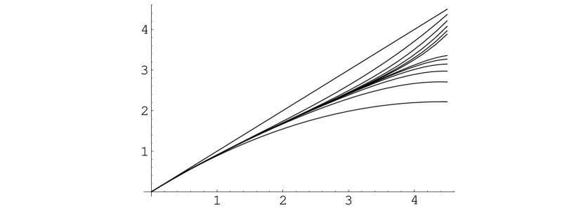
FIG. 3.: Plot of partial sums ($S_{n}$) of the series of Eq. (34) as functions of $P_{1}$, keeping $a=0.3$ for $n=1,\ldots,12$. The thick line formed by the partial sums corresponds to the true value of ${\tilde{N}}(k,Y)$. The straight line represents the single BFKL pomeron exchange contribution.

To find the radius of convergence and the high energy asymptotic behavior of the series in Eq. (34) let us study the terms corresponding to large values of $n$. These terms describe the multiple pomeron exchange contributions. We would like to explore very large $n$, such that $n^{2}a(k,Y)\gg 1$. Then the coefficients $a_{n}$ determining the recursion relations in (35) for the coefficients of the series become

$$a_{n}=-\frac{1}{n\,4\,\ln 2}.$$ (37)

Thus, redefining

$$f_{n}=\left(\frac{-1}{4\,\ln 2}\right)^{n-1}\tilde{f}_{n},$$ (38)

we obtain the following recursion relations instead of Eq. (35)

$$\tilde{f}_{n}=\frac{1}{n}\sum_{m=1}^{n-1}\,\tilde{f}_{m}\,\tilde{f}_{n-m},\hskip 28.45274pt\mbox{large}\,n.$$ (39)

For very large $n$ Eq. (39) could be satisfied up to order $1/n$ corrections with the ansatz

$$\tilde{f}_{n}=\left(\frac{1}{r}\right)^{n}+o\left(\frac{1}{n}\right),$$ (40)

where $r$ could be some arbitrary constant. Here we have to point out that since Eq. (39) is written for very large $n$ we can not use $f_{1}=1$ as a “normalization” condition anymore and that way we have lost the information which would have allowed us to fix the value of $r$. In principle $r$ should depend on $a(k,Y)$, but this function is a much slower varying function of $k$ and $Y$ than $P_{1}(k,Y)$, so we assume $r$ to be constant in our analysis. If we fix $\tilde{f}_{1}=1$ then numerical estimates show that $r\approx 1.4$, which allows one to hope that for asymptotics of Eq. (35) $r$ is not very large and does not introduce a large correction to our analysis.

Using the ansatz of Eq. (40) together with Eq. (38) in Eq. (34) we conclude that the constructed perturbation series is convergent as long as

$$\frac{P_{1}(k,Y)}{r\,4\,\ln 2}<1.$$ (41)

Outside the region specified by the condition of Eq. (41) the series in Eq. (34) is not convergent anymore. Multiple pomeron exchange contributions corresponding to large values of $n$ become much larger and, consequently, more important than the one- or two-pomeron exchanges. Defining the saturation momentum scale $Q_{s}$ by the following condition

$$\frac{P_{1}(Q_{s},Y)}{r\,4\,\ln 2}=1$$ (42)

we obtain (for not very large $Q_{s}$) [27]

$$Q_{s}(Y)=\Lambda\,\frac{C_{-1}}{r\,4\,\ln 2}\,\frac{\exp[(\alpha_{P}-1)Y]}{\sqrt{14\alpha N_{c}\zeta(3)Y}}.$$ (43)

Using this quantity we can say that for the transverse momenta of the quark–antiquark pair greater than the saturation momentum, $k>Q_{s}$, the series converges. For the transverse momenta below the saturation scale, $k<Q_{s}$, that is, inside the saturation region, the series diverges ceasing to be a reliable approximation to the solution of Eq. (14).

One might wonder whether the condition $\ln^{2}(k/\Lambda)>\alpha N_{c}Y$, which we needed to perform the saddle point integrations above, would prevent us from exploring the high energy asymptotics with the series of Eq. (34) by putting an upper limit on the possible values of $Y$ for fixed $k$. Really, this condition provides us with the limit on the range of rapidities for the perturbative solution we found

$$Y<Y_{sp}\sim\frac{1}{\alpha N_{c}}\,\ln^{2}\frac{k}{\Lambda}.$$ (44)

However we also have to note that the series (34) is convergent as long as $k>Q_{s}(Y)\sim\alpha^{2}\Lambda e^{(\alpha_{P}-1)Y}$, i.e., outside of the saturation region. This yields us with another constraint on $Y$

$$Y<Y_{sat}\sim\frac{1}{\alpha_{P}-1}\,\ln\frac{k}{\alpha^{2}\Lambda}.$$ (45)

Now one can see that the two conditions (44) and (45) are roughly of the same order of magnitude. Thus the condition $\ln^{2}(k/\Lambda)>\alpha N_{c}Y$ does not impose any additional constraint on the kinematic region of the applicability of the series in Eq. (34) since the series diverges in the region where the condition is violated anyway.

Now we want to find some approximation to the solution of Eq. (14) inside the saturation region. The saturation region is specified by the condition that $k<Q_{s}(Y)$ and could be achieved either by decreasing the transverse momentum or by increasing the center of mass energy of the system.

First we note that one may find a correction to Eq. (40). Rewriting it as

$$\tilde{f}_{n}=\tilde{f}_{n}^{(0)}+\epsilon_{n},$$ (46)

where $\tilde{f}_{n}^{(0)}=(1/r)^{n}$ for large $n$ and $\tilde{f}_{n}^{(0)}\sim a^{n/2}\ll 1$ for small $n$, i.e., it satisfies Eq. (35) with the large $n$ asymptotics given by leading in $n$ behavior of Eq. (40). Substituting Eq. (46) into Eq. (40), expanding it to the lowest order in $\epsilon_{n}$ and neglecting $\tilde{f}_{n}^{(0)}$ for small values of $n$ one obtains

$$\epsilon_{n}\sim\frac{1}{n}\,\left(\frac{1}{r}\right)^{n}.$$ (47)

Using Eqs. (47), (40) and (38) in (34) we could sum up leading in $n$ terms of the series (34) obtaining some expressions which could be analytically continued outside the region of convergence of the series of Eq. (34). This way we might obtain an expression for the solution of Eq. (14) inside the saturation region, that is for large $P_{1}$. While the leading in $n$ part of the series given by Eq. (40) gives a function which goes to a constant for large $P_{1}$, the subleading terms given by Eq. (47) yield us with

$$\sum_{n=1}^{\infty}\frac{(-1)^{n-1}}{n}\,\left(\frac{P_{1}}{r\,4\,\ln 2}\right)^{n}=\ln\left(1+\frac{P_{1}}{r\,4\,\ln 2}\right).$$ (48)

Analytically continuing $\ln(1+\frac{P_{1}}{r\,4\,\ln 2})$ in the region of large $P_{1}$ we obtain for asymptotically large energies $\ln\frac{P_{1}}{r\,4\,\ln 2}$. Of course we do not know whether the higher order corrections in $1/n$ would not give us some other function of $P_{1}$ which would be large for large $P_{1}$ possibly interfering with our $\ln P_{1}$ ansatz. Therefore $\ln P_{1}$ should be considered only as a a possible high energy asymptotics of $\tilde{N}$ and the above argument should not be taken as a proof of this statement.

To justify that the above ansatz of $\tilde{N}=\ln\frac{P_{1}}{r\,4\,\ln 2}=\ln\frac{Q_{s}}{k}$ is the solution of Eq. (14) at asymptotically high energies we first note that

$$\tilde{N}(k,Y)=\ln\frac{M}{k},$$ (49)

with $M$ some large momentum scale ($k<M$) satisfies the equation

$$2\,\chi\left(-\frac{\partial}{\partial\ln k}\right)\,{\tilde{N}}(k,Y)-{\tilde{N}}^{2}(k,Y)=0.$$ (50)

Really, rewriting

$$\ln\frac{M}{k}=-\int_{C}\frac{d\lambda}{2\pi i}\,\frac{1}{\lambda^{2}}\left(\frac{k}{M}\right)^{\lambda},$$ (51)

where the contour $C$ is a circle of radius less than one centered around $\lambda=0$, one can see that since $\chi(-\lambda)$ also has a pole at $\lambda=0$ then

$$2\,\chi\left(-\frac{\partial}{\partial\ln k}\right)\,\ln\frac{M}{k}=\ln^{2}\frac{M}{k}.$$ (52)

We can assume that in the saturation region $\tilde{N}(k,Y)$ ceases to depend on $Y$. Then Eq. (14) reduces to Eq. (50). To find the most general solution of Eq. (50) we represent $\tilde{N}$ as a series

$$\tilde{N}(k,Y)=\sum_{n,m=0}^{\infty}c_{nm}\left(\frac{k}{M}\right)^{n}\,\ln^{m}\frac{M}{k}$$ (53)

and substitute it into Eq. (50) in order to find the unknown coefficients $c_{nm}$. Using the technique outlined above for $\ln\frac{M}{k}$ we can show that

$$2\,\chi\left(-\frac{\partial}{\partial\ln k}\right)\,\left[\left(\frac{k}{M}\right)^{n}\,\ln^{m}\frac{M}{k}\right]=\left\{\begin{array}[]{c}\frac{2}{m+1}\left(\frac{k}{M}\right)^{n}\,\ln^{m+1}\frac{M}{k},\hskip 28.45274pt\mbox{even}\,\,n,\\ \\ 2\,\chi(-n)\left(\frac{k}{M}\right)^{n}\,\ln^{m}\frac{M}{k},\hskip 28.45274pt\mbox{odd}\,\,n.\end{array}\right.$$ (54)

With the help of Eq. (54) one can show that in order for the series of Eq. (53) to satisfy Eq. (50) all of its coefficients must be zero with the exception of $c_{01}=1$. Thus we proved that the most general energy independent solution of Eq. (14) is given by Eq. (49).

At asymptotically high energies there is only one large momentum scale in the scattering of the quark–antiquark pair on a hadron or nucleus — the saturation scale $Q_{s}$. This scale is also suggested by the ansatz of Eq. (48). Therefore we should put $M=Q_{s}$ and use Eq. (49) as a solution of Eq. (14) in the region when $k<Q_{s}$. The derivative of this new solution with respect to rapidity is of the order of $\partial\ln(Q_{s}/k)/\partial Y\sim\alpha N_{c}$ and could be neglected compared to any of the terms on the right hand side of Eq. (14), each of them being of the order of $\alpha N_{c}(\alpha N_{c}Y)^{2}$. This could be done since $\alpha N_{c}Y\gg 1$. Therefore we conclude that in the saturation region

$$\tilde{N}(k,Y)\approx\ln\frac{Q_{s}}{k},\hskip 28.45274ptY\geq\frac{1}{\alpha_{P}-1}\,\ln\,\frac{1}{\alpha^{2}}.$$ (55)

Now that we know the solution for $\tilde{N}(k,Y)$ outside of the saturation region given by Eqs. (34), (35) and (36) and the high energy asymptotics inside the saturation region given by Eq. (55), one might want to construct the solution in coordinate space ($N(x_{\perp},Y)$) using the Fourier transformation of Eq. (12). To do that one would have to integrate over all values of the transverse momentum $k$ from $0$ to $\infty$. If $x_{\perp}<1/Q_{s}$ then the transverse momentum, which in Eq. (12) is effectively cut off by the Bessel function and , therefore, varies approximately from $0$ to $1/x_{\perp}>Q_{s}$, will go through a range of values both above and below $Q_{s}$. For the first case one would have to use the perturbation series which we constructed as $\tilde{N}$, while for the second case one might use the asymptotic value of $\tilde{N}$ given by Eq. (55) , although a perturbative expansion around it would be more accurate. The result would be a complicated combination of special function and we are not going to list it here.

If $x_{\perp}>1/Q_{s}$ then the transverse momentum in Eq. (12) simply gets cut off by $1/x_{\perp}<Q_{s}$ and always stays within the saturation region. Thus one could just perform a Fourier transformation of formula (55) using Eq. (12). The result is

$$N(x_{\perp},Y)\approx 1,\hskip 28.45274ptY\geq\frac{1}{\alpha_{P}-1}\,\ln\,\frac{1}{\alpha^{2}}.$$ (56)

This corresponds to the blackness of the total cross section of the quark–antiquark pair on the target nucleus, since it is given by

$$\sigma_{q\overline{q}A}^{tot}=2\,\int d^{2}b_{0}N(x_{\perp},b_{0},Y)\approx 2\pi R^{2}$$ (57)

for $N=1$ and for a cylindrical nucleus of radius $R$ as described above. That way the total cross section is independent of energy at asymptotically high energies and is completely unitary. It reaches its “geometrical” limit (57) which could be predicted even from quantum mechanics.

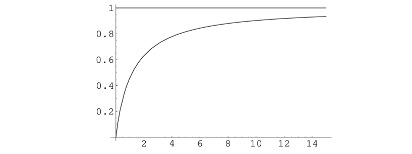
FIG. 4.: Plot of the qualitative behavior of the forward $q\overline{q}$ pair scattering amplitude on a nucleus, $N(x_{\perp},Y)$ , as a function of $x_{\perp}Q_{s}(Y)$ (one BFKL pomeron exchange contribution). At small values of $x_{\perp}Q_{s}$ the structure function is linear in $x_{\perp}Q_{s}$, reproducing BFKL pomeron. As energy increases the forward amplitude $N$ saturates to a constant.

That way we have shown that $N(x_{\perp},Y)$ given by the solution of Eq. (14) behaves like a single BFKL pomeron exchange contribution at moderately high energies ($Y\sim 1/\alpha$), which follows from the perturbation series we have constructed, and as energy increases to very high quantities ($Y\geq\frac{1}{\alpha_{P}-1}\,\ln\,\frac{1}{\alpha^{2}}$), saturates to a constant independent of energy. A qualitative sketch of $N(x_{\perp},Y)$ as a function of $x_{\perp}Q_{s}(Y)$ (one pomeron contribution) is shown in Fig. 4.

III Asymptotic behavior of the $F_{2}$ structure function

For a large cylindrical nucleus the $F_{2}$ structure function is given by

$$F_{2}(x,Q^{2})=\frac{Q^{2}R^{2}}{8\pi^{2}\alpha_{EM}}\int d^{2}x_{01}\,dz\,\Phi(x_{01},z)\,N(x_{01},Y),$$ (58)

which follows from Eq. (3). We can rewrite Eq. (58) in momentum space using Eq. (12)

$$F_{2}(x,Q^{2})=\frac{Q^{2}R^{2}}{4\pi\alpha_{EM}}\int d^{2}k\,dz\,\tilde{\Phi}(k,z)\,\tilde{N}(k,Y),$$ (59)

where

$$\tilde{\Phi}(k,z)=\int\frac{d^{2}x_{01}}{(2\pi)^{2}}\,e^{i{\bf k}\cdot{\bf x}_{01}}\,x^{2}_{01}\,\Phi(x_{01},z).$$ (60)

Employing Eqs. (6) and (7) we obtain

$$\tilde{\Phi}(k,z)=\frac{\alpha_{EM}N_{c}}{\pi^{2}}\left\{[z^{2}+(1-z)^{2}]\,\frac{2}{3a^{2}}\,_{2}F_{1}\left(2,3,2.5,-\frac{k^{2}}{4a^{2}}\right)+\right.$$

$$\left.+4\,Q^{2}\,z^{2}(1-z)^{2}\,\frac{1}{15a^{6}}\,\left[5\,a^{2}\,_{2}F_{1}\left(2,2,2.5,-\frac{k^{2}}{4a^{2}}\right)-2\,k^{2}\,_{2}F_{1}\left(3,3,3.5,-\frac{k^{2}}{4a^{2}}\right)\right]\right\},$$ (61)

where ${}_{2}F_{1}$ is a hypergeometric function.

Eq. (59) shows that in order to write down an expression for the $F_{2}$ structure function one has to know $\tilde{N}(k,Y)$ in the areas above and below saturation. The situation is similar to the Fourier transformation of the previous section. The wave function $\tilde{\Phi}(k,z)$ given by Eq. (61) becomes very small for transverse momenta $k>a=Q\sqrt{z(1-z)}$, effectively providing an upper cutoff on the $k$ integration. Thus if $Q>Q_{s}$ the integral over $k$ includes $k<Q_{s}$ and $k>Q_{s}$ and to calculate it we have to use the solution for $\tilde{N}$ both inside and outside of the saturation region. We can again propose the approximation outlined in Sect. II for calculation of $F_{2}$, which consists of using perturbation series of Eq. (34) outside saturation region and approximating the solution inside that region by Eq. (55). The result would also include a complicated list of special functions which we are not going to list here. We have to admit that numerical solution of Eq. (8) could give a more precise results for $F_{2}$. Here we can just point out that at moderately high energies the behavior of the $F_{2}$ structure function will be dominated by single BFKL pomeron exchange, providing us with the following formula which could be obtained by substituting the first term in the series of Eq. (34) into Eq. (59)

$$F_{2}(x,Q^{2})=\frac{11}{256}\,S_{\perp}N_{c}Q\Lambda\,\frac{C_{-1}}{4\,\ln 2}\,\frac{\exp[(\alpha_{P}-1)Y]}{\sqrt{14\alpha N_{c}\zeta(3)Y}},\hskip 28.45274ptY\sim\frac{1}{\alpha},$$ (62)

where we have neglected the transverse momentum diffusion term in the exponent of Eq. (22) and $S_{\perp}=\pi R^{2}$. Eq. (62) is valid only for moderately high energies, when the saturation momentum $Q_{s}$ is small and we can neglect the $k$ integration in Eq. (59) below that scale.

When $Q<Q_{s}$ or the energy gets very high to sufficiently increase $Q_{s}$ the integral over $k$ in Eq. (59) is limited to $k<Q<Q_{s}$, so that we can use Eq. (55) for $\tilde{N}(k,Y)$. The result yields

$$F_{2}(x,Q^{2})=\frac{Q^{2}R^{2}N_{c}}{3\pi^{2}}\,\left(\ln\frac{Q_{s}}{Q}+\frac{13}{12}\right),\hskip 28.45274ptQ<Q_{s}.$$ (63)

As energy becomes very large, corresponding to $Y\sim\frac{1}{\alpha_{P}-1}\ln\frac{1}{\alpha^{2}}$, $\ln\frac{Q_{s}}{Q}$ becomes approximately equal to $(\alpha_{P}-1)Y$. Therefore

$$F_{2}(x,Q^{2})\approx\frac{Q^{2}R^{2}N_{c}}{3\pi^{2}}\,(\alpha_{P}-1)Y,\hskip 28.45274ptY\geq\frac{1}{\alpha_{P}-1}\ln\frac{1}{\alpha^{2}}.$$ (64)

We conclude that $F_{2}\sim\ln s$ at asymptotically high energies. This conclusion may seem to be a little unusual, so we will reproduce the same result using more conventional coordinate space language. As was shown in the previous section the forward amplitude of the $q\overline{q}$ pair scattering on a nucleus is $N(x_{\perp},Y)=1$, when $x_{\perp}>1/Q_{s}$. When $x_{\perp}<1/Q_{s}$ one could argue that the amplitude is roughly proportional to some positive power of $x_{\perp}$, at least $N(x_{\perp},Y)\sim x_{\perp}$, as given by one pomeron exchange. Thus, for $Q<Q_{s}$ we can neglect the part of the integral with $x_{01}<1/Q_{s}$ in Eq. (58), since the wave function $\Phi$ in Eq. (58) behaves like $\frac{1}{x_{01}^{2}}$ and is not singular enough to make that portion of the integral significant. That way, expanding the modified Bessel functions in $\Phi$ of Eq. (6) and integrating over $z$ we obtain

$$F_{2}(x,Q^{2})\approx\frac{Q^{2}R^{2}N_{c}}{3\pi^{2}}\,\int_{1/Q_{s}}^{1/Q}\,\frac{dx_{01}}{x_{01}}.$$ (65)

The upper cutoff on the $x_{01}$ integration in Eq. (65) is provided by the fact that the modified Bessel functions fall off exponentially at the large values of the argument. Integrating over $x_{01}$ in Eq. (65) we arrive at Eq. (64).

That way we have shown that the $F_{2}$ structure function given by the solution of Eq. (33) is proportional to the single BFKL pomeron exchange contribution (62) at moderately high energies with $Y\sim 1/\alpha$, and, as energy increases the $F_{2}$ structure function unitarizes, becoming linearly proportional to $\ln s$ (64). We stress again that even though the cross section of the quark–antiquark pair of a fixed transverse size $x_{\perp}$ scattering on a nucleus saturates to a constant at large $Y$, the integral over $x_{\perp}$ makes $F_{2}$ depend on $Y$, such that $F_{2}\sim Y$ at very large $Y$.

IV Application to diffraction

In [25] a diffractive deep inelastic scattering process was considered, an amplitude of which is shown in Fig. 5. A virtual photon scatters on a nucleus elastically, leaving it intact. Two quarks in the final state in Fig. 5 may become a pair of jets or form a vector meson. These type of processes were called quasi–elastic virtual photoproduction in [25].

FIG. 5.: Quasi–elastic deep inelastic scattering as pictured in [25].

The interactions between the quark–antiquark pair and the nucleus were taken in the quasi–classical approximation, similar to [28]. Each nucleon in [25] would interact with the $q\overline{q}$ pair by a two gluon exchange. Strictly speaking this approximation corresponds to not very high energies, when the logarithms of $s$ resulting from QCD evolution are not large enough to become important. That is why the approximation is called quasi–classical. In [25] it provided us with a simple Glauber type expression for the diffractive, or, more correctly, quasi–elastic structure function $F_{2}^{D}$ [cf. Eq. (20) in [25]]

$$F_{2}^{D}(x,Q^{2})=\frac{Q^{2}N_{c}}{\pi(2\pi)^{3}}\int d^{2}b_{0}\,\,d^{2}x_{01}\,\int_{0}^{1}dz\left\{a^{2}K_{1}^{2}(x_{01}a)[z^{2}+(1-z)^{2}]+4Q^{2}z^{2}(1-z)^{2}K_{0}^{2}(x_{01}a)\right\}$$

$$\times\gamma^{2}({\bf x}_{01},{\bf b}_{0}),$$ (66)

where we again assumed that the quarks are massless and have only one flavor. $\gamma({\bf x}_{01},{\bf b}_{0})$ is the Glauber propagator of the quark–antiquark pair, which for the case of a cylindrical nucleus is given by Eq. (9). One can obtain Eq. (66) from Eq. (3) by first noting that the quasi–classical limit corresponds to putting $Y=0$ (no evolution in rapidity) in it and $N({\bf x}_{01},{\bf b}_{0},Y=0)=\gamma({\bf x}_{01},{\bf b}_{0})$. Recalling that, as was argued in [25], one can rewrite the total and elastic cross sections for DIS on a nucleus in terms of the $S$-matrix at a given impact parameter of the collision, $S(b)$, yielding

$$\sigma_{tot}=2\int d^{2}b\,\,[1-S(b)]$$ (68)

$$\sigma_{el}=\int d^{2}b\,\,[1-S(b)]^{2}$$ (69)

and associating $F_{2}$ with $\sigma_{tot}$ and $F_{2}^{D}$ with $\sigma_{el}$, we can easily derive Eq. (66) from Eq. (3) [25].

Now let us imagine our quasi–elastic process at very high energies. Then, strictly speaking, one has to include the evolution in rapidity in the structure function $F_{2}^{D}$. We still do not want to have particles being produced in the central rapidity region. One could model the interaction by a single pomeron exchange between the quark–antiquark pair and the nucleus, similarly to what was done previously in [29] and references mentioned there for elastic scattering. Here we are going to propose inclusion of multiple pomeron exchanges in $F_{2}^{D}$. Since the above formalism allows us to sum up pomeron fan diagrams in the leading logarithmic approximation, we can just insert this evolution in the amplitude of the quasi–elastic process. The diagram of the process is depicted in Fig. 6. The diffractive rapidity gap between the nucleus in the final state and the remains of the $q\overline{q}$ pair results not only from a single pomeron exchange, but also from multiple pomeron exchanges. Still nothing is produced in the central rapidity region.

FIG. 6.: Quasi–elastic scattering including multiple pomeron exchanges, as envisioned in our approach.

The corresponding expression for the diffractive structure function $F_{2}^{D}$ is easy to derive. We know the expression for the total $F_{2}$ structure function in Eq. (3), which includes all the discussed multiple pomeron exchanges. One can easily argue along the lines outlined in deriving Eq. (66), that for the case of multiple pomeron exchanges we again have a relationship between the total and elastic cross sections similar to the one given by Eqs. (68) and (69). That way we conclude that to obtain a formula for $F_{2}^{D}$ one has to substitute $\gamma({\bf x}_{01},{\bf b}_{0})$ in Eq. (66) with $N({\bf x}_{01},{\bf b}_{0},Y)$. The result is

$$F_{2}^{D}(x,Q^{2})=\frac{Q^{2}N_{c}}{\pi(2\pi)^{3}}\int d^{2}b_{0}\,\,d^{2}x_{01}\,\int_{0}^{1}dz\left\{a^{2}K_{1}^{2}(x_{01}a)[z^{2}+(1-z)^{2}]+4Q^{2}z^{2}(1-z)^{2}K_{0}^{2}(x_{01}a)\right\}$$

$$\times\,N^{2}({\bf x}_{01},{\bf b}_{0},Y),$$ (70)

where $N({\bf x}_{01},{\bf b}_{0},Y)$ is, in the large $N_{c}$ limit, a solution of Eq. (8). Eq. (70) is our master formula for the diffractive (quasi–elastic) structure function. When $Y=0$ (no evolution) it reduces to Eq. (66).

Using the results of Sect. II we can derive the asymptotics of the diffractive structure function. At moderately high energies the one pomeron exchange contribution dominates the diffractive amplitude of Fig. 6. Again, similar to the previous section we assume that since at $Y\sim 1/\alpha$ the saturation scale $Q_{s}$ is small one can neglect the $k$ integration below $Q_{s}$. Performing a Fourier transformation (12) of the first term in the series of Eq. (34) and substituting the result into Eq. (70) we obtain for a cylindrical nucleus

$$F_{2}^{D}(x,Q^{2})=\frac{S_{\perp}N_{c}\Lambda^{2}}{3\pi^{3}}\,\frac{C_{-1}^{2}}{(4\,\ln 2)^{2}}\,\frac{\exp[2(\alpha_{P}-1)Y]}{14\alpha N_{c}\zeta(3)Y}\,Y,\hskip 28.45274ptY\sim\frac{1}{\alpha},$$ (71)

where we had to cut off the $z$ integral in Eq. (70) by $e^{-Y}$ and we again neglected the transverse momentum diffusion term in Eq. (22). The diffractive structure function of Eq. (71) behaves like a square of a single pomeron exchange contribution, similar to what was found for elastic parton scattering in [29]. Even though $F_{2}^{D}\sim Q_{s}^{2}(Y)$ in Eq. (71) is growing with energy faster than $F_{2}\sim Q_{s}(Y)$ in Eq. (62), unitarity is not violated, since both expressions are valid in the region of relatively small $Q_{s}$ corresponding to $Y\sim 1/\alpha$. Thus at moderate energies $F_{2}^{D}\ll F_{2}$, as $Q_{s}\ll\Lambda$.

We also note that formula (71) was derived assuming that the photon’s virtuality $Q^{2}$ is not very large. Therefore, the fact that $F_{2}^{D}$ in Eq. (71) has no powers of $Q$ in the numerator, whereas the corresponding $F_{2}$ given by Eq. (62) is proportional to $Q$, does not imply that $F_{2}^{D}$ is not a leading twist effect, violating the theoretical predictions [25, 30] and experimental observations [31]. For the case of large $Q$ one should perform a different saddle point approximation for the terms in the perturbative series given by Eqs. (19), (26), etc., [see [32]], getting a different series solving Eq. (14) outside of the saturation region. This should result in concluding that $F_{2}^{D}$ given by the first term in that series is not suppressed by any powers of $Q$ compared to $F_{2}$. However, doing that is beyond the scope of this paper.

At very high energies, when $Q_{s}(Y)$ is large enough so that $Q<Q_{s}(Y)$, the quasi–elastic structure function $F_{2}^{D}$ saturates. Similarly to Sect. III we can derive the high energy asymptotic behavior of Eq. (70). Putting $N(x_{01},Y)=1$ for $x_{01}>1/Q_{s}$ and imposing the cutoffs on the $x_{01}$ integration in Eq. (70) analogously to what was done in deriving Eq. (65) we deduce

$$F_{2}^{D}(x,Q^{2})\approx\frac{Q^{2}R^{2}N_{c}}{6\pi^{2}}\,(\alpha_{P}-1)Y,\hskip 28.45274ptY\geq\frac{1}{\alpha_{P}-1}\ln\frac{1}{\alpha^{2}}.$$ (72)

That way the $F_{2}^{D}$ also becomes linearly proportional to the logarithm of center of mass energy energy at very high energies, similarly to the total structure function $F_{2}$. Comparing Eq. (72) with the high energy behavior of the $F_{2}$ structure function given by Eq. (64) we conclude that $F_{2}^{D}$ is still smaller than $F_{2}$ and unitarity is again not violated. One can see that at this asymptotically high energy $F_{2}=2F_{2}^{D}$, which corresponds to the prediction for the black cross sections resulting from quantum mechanics.

V Conclusions

In this paper we have found a solution of the evolution equation (8) which resums all pomeron fan diagrams in the leading logarithmic limit for large $N_{c}$, that was proposed in [1]. The solution consists of two parts. Outside of the saturation region we have constructed a perturbative series in momentum space given by Eqs. (34), (35) and (36). We have demonstrated that the series tends to unitarize the single BFKL pomeron exchange contribution (see Fig. 3). In deriving formula (14), which led to Eqs. (34), (35) and (36), we had to assume that DIS cross sections are slowly varying functions of the impact parameter, which corresponds to scattering on a large nucleus. Only in the large nucleus case we could argue that the fan diagrams dominate the total DIS cross sections. In order to perform the saddle point approximation in Eqs. (19), (26), (31) and for the series (34) to be convergent we had to assume that $\ln(Q/\Lambda)\ll\alpha N_{c}Y$ and $Q>Q_{s}(Y)$, restricting the possible values of $Q$ to a certain not very broad range. Nevertheless the abovementioned assumptions did not change the qualitative behavior of the obtained result and the conclusions could be easily extended to large $Q$ by performing a different saddle point approximation.

Inside the saturation region, for $Q<Q_{s}$, we found an approximate solution given by Eq. (55) corresponding to the saturation of the total scattering cross section of a quark–antiquark pair of a given transverse size on a nucleus to a constant independent of energy (56). That way we have shown that the coordinate space forward amplitude of the $q\overline{q}$ scattering on a nucleus or hadron grows like a BFKL pomeron exchange contribution at moderately high energies (22), and, as energy gets very large it saturates to a constant (56). A qualitative plot of $N(x_{\perp},Y)$ is presented in Fig. 4.

We have to admit that in order to construct a solution of Eq. (8) in coordinate space, $N(x_{\perp},Y)$, and the corresponding structure function $F_{2}$ one has to have a better knowledge of the momentum space solution inside the saturation region. A numerical solution of Eq. (8) would probably be very helpful in determining exact values of $N(x_{\perp},Y)$ and $F_{2}$ at intermediately large rapidities.

We have shown that the $F_{2}$ structure function given by the solution of Eq. (8) grows as a power of energy at moderately high energies, corresponding to rapidities of the order of $Y\sim 1/\alpha$. This behavior, presented in Eq. (62), reproduces the usual single BFKL pomeron exchange contribution to the structure function. As energy grows very high, corresponding to the rapidities of the order of $Y{{}_{\displaystyle{>}}\atop\displaystyle{\sim}}[1/(\alpha_{P}-1)]\ln(1/\alpha^{2})$, the $F_{2}$ structure functions unitarizes, becoming linearly proportional to $\ln s$, which satisfies Froissart bound. This is shown in Eq. (64). Thus we have shown that the BFKL pomeron on the nucleus is unitarized by summation of pomeron fan diagrams.

We also note that we derived an expression for the quasi–elastic (diffractive) structure function $F_{2}^{D}$ presented in Eq. (70), which also includes all multiple pomeron exchanges. We have shown that at moderately high energies the obtained expression behaves like a square of the BFKL pomeron contribution [Eq. (71)] and at very high energies it saturates and becomes a linear function of $\ln s$ [Eq. (72)], being equal to a half of the structure function $F_{2}$, as expected for black cross sections.

In [1] it was argued that the dipole model provides us with the techniques that allow one to resum pomeron fan diagrams at any subleading logarithmic order in the large $N_{c}$ limit. That is, if one calculates the next-to-leading order kernel in the dipole model, the resulting equation for the generating functional $Z$ [see [11, 12, 13]] would provide us with the equation resumming all NLO pomeron fan diagrams. The resulting equation would be, probably, more complicated than our Eq. (8). It would have a much more sophisticated kernel [7, 8] and would have cubic terms in $N$ on the right hand side. However, the analysis presented in this paper allows one to hope that this resummation will cure some of the problems of the recently calculated NLO BFKL kernel [9]. Resummation of one loop running coupling corrections, which are a part of the NLO BFKL kernel, brings a factor of $e^{c\alpha^{5}Y^{3}}$ in the one pomeron exchange amplitude, with the constant $c\approx 5$ for three flavors [9]. Since it introduces an even faster growth with energy than the leading order BFKL pomeron, this factor seems to complicate the problem of unitarization of the pomeron. However, the inclusion if this factor of $e^{c\alpha^{5}Y^{3}}$ in our definition of $P_{1}$ in Eq. (22) would not change the perturbation series of Eq. (34) and the quark–antiquark scattering amplitude would still be unitarized by multiple pomeron exchanges. Of course a careful inclusion of higher order corrections would lead to much more complicated results. Nevertheless we may hope that inclusion of one loop running coupling corrections would just modify the one pomeron exchange contribution and the multiple pomeron exchanges would still unitarize the total DIS cross section. However, a rigorous proof of this statement is beyond our goals here.

Finally we point out that one can use the developed technique to construct a gluon distribution function $xG(x,Q^{2})$ of the nucleus including multiple hard pomeron exchanges similarly to the way we have constructed the $F_{2}$ structure function. To do that one has to consider scattering of the “current” $j=-(1/4)F^{a}_{\mu\nu}F^{a}_{\mu\nu}$ on the nucleus, similarly to [17, 27, 28]. Then, in the large $N_{c}$ limit, it should be possible to derive an equation for the generating functional of the dipole wave function of the current $j$, which, at the end, would provide us with an expression for the gluon distribution function $xG(x,Q^{2})$.

After this paper was finished the author has learned about another effort to solve Eq. (8) which was carried out in [33].

A

Here we are going to show how the Fourier transformation of Eqs. (12) and (13) reduces Eq. (10) to Eq. (14). First we note that [11, 34]

$$d^{2}x_{2}=2\pi\,x_{12}\,x_{02}\,dx_{12}\,dx_{02}\,\int_{0}^{\infty}dk\,k\,J_{0}(kx_{01})\,J_{0}(kx_{02})\,J_{0}(kx_{12}),$$ (A1)

which would allow us to integrate independently over $x_{02}$ and $x_{12}$ in the kernel of Eq. (10). Using the Jacobian of Eq. (A1) in the second (quadratic) term on the right hand side of Eq. (10), multiplying both sides of Eq. (10) by $J_{0}(kx_{01})/x_{01}$, integrating over $x_{01}$ from $0$ to $\infty$ and employing

$$\int_{0}^{\infty}dx\,x\,J_{0}(kx)J_{0}(k^{\prime}x)=\frac{1}{k}\delta(k-k^{\prime})$$ (A2)

we obtain

$$\frac{\partial{\tilde{N}}(k,Y)}{\partial Y}=\frac{\alpha N_{c}}{\pi^{2}}\int_{0}^{\infty}\frac{dx_{01}}{x_{01}}J_{0}(kx_{01})\int_{\rho}d^{2}x_{2}\left[\frac{x^{2}_{01}}{x^{2}_{02}x^{2}_{12}}-2\pi\delta^{2}({\bf x}_{01}-{\bf x}_{02})\ln\left(\frac{x_{01}}{\rho}\right)\right]N({\bf x}_{02},Y)$$

$$-\frac{\alpha N_{c}}{\pi}{\tilde{N}}^{2}(k,Y).$$ (A3)

The first (linear in $N$) term on the right hand side of Eq. (A3) can be rewritten employing Eqs. (A1), (12) and (13) as

$$\frac{2\alpha N_{c}}{\pi}\int_{0}^{\infty}dk^{\prime}\,k^{\prime}\,{\tilde{N}}(k^{\prime},Y)\int_{0}^{\infty}dx_{01}\,x_{01}\,J_{0}(kx_{01})\,J_{0}(k^{\prime}x_{01})\,\left(\int_{\rho}^{\infty}\,\frac{dx_{12}}{x_{12}}\,J_{0}(k^{\prime}x_{12})-\ln\frac{x_{01}}{\rho}\right).$$ (A4)

Using the techniques outlined in Eqs. (32) and (33) of [11] the integral in the parenthesis of Eq. (A4) can be done, yielding

$$\int_{\rho}^{\infty}\,\frac{dx_{12}}{x_{12}}\,J_{0}(k^{\prime}x_{12})=\psi(1)-\ln\frac{k^{\prime}\rho}{2}.$$ (A5)

Substituting this back into Eq. (A4) we end up with

$$\frac{2\alpha N_{c}}{\pi}\int_{0}^{\infty}dk^{\prime}\,k^{\prime}\,{\tilde{N}}(k^{\prime},Y)\int_{0}^{\infty}dx_{01}\,x_{01}\,J_{0}(kx_{01})\,J_{0}(k^{\prime}x_{01})\,\left(\psi(1)-\ln\frac{k^{\prime}x_{01}}{2}\right).$$ (A6)

Expanding $J_{0}(kx_{01})$ in a Taylor series we rewrite Eq. (A6) as

$$\frac{2\alpha N_{c}}{\pi}\int_{0}^{\infty}dk^{\prime}\,k^{\prime}\,{\tilde{N}}(k^{\prime},Y)\sum_{m=0}^{\infty}\frac{(-1)^{m}}{(m!)^{2}}\left(\psi(1)-\frac{\partial}{\partial(2m)}\right)\left[\left(\frac{k}{2}\right)^{2m}\int_{0}^{\infty}dx_{01}\,x_{01}J_{0}(k^{\prime}x_{01})\,x_{01}^{2m}\right].$$ (A7)

Performing the integration over $x_{01}$ in Eq. (A7) we obtain [ see Eq. (33) in [11]]

$$\frac{2\alpha N_{c}}{\pi}\int_{0}^{\infty}\frac{dk^{\prime}}{k^{\prime}}\,{\tilde{N}}(k^{\prime},Y)\sum_{m=0}^{\infty}\frac{(-1)^{m}}{(m!)^{2}}\left(\psi(1)-\frac{\partial}{\partial(2m)}\right)\left[2\left(\frac{k}{k^{\prime}}\right)^{2m}\frac{\Gamma(m+1)}{\Gamma(-m)}\right].$$ (A8)

After differentiating over $m$ and employing the fact that

$$\sum_{m=0}^{\infty}\frac{(-1)^{m}}{m!}\left(\frac{k}{k^{\prime}}\right)^{2m}\frac{1}{\Gamma(-m)}=\frac{k}{2}\,\delta(k-k^{\prime}),$$ (A9)

which is a direct consequence of Eq. (A2), we can reduce Eq. (A8) to

$$\frac{2\alpha N_{c}}{\pi}\int_{0}^{\infty}\frac{dk^{\prime}}{k^{\prime}}\,{\tilde{N}}(k^{\prime},Y)\sum_{m=0}^{\infty}\frac{(-1)^{m}}{m!}\,2\chi(-2m)\left(\frac{k}{k^{\prime}}\right)^{2m}\frac{1}{\Gamma(-m)},$$ (A10)

with $\chi$ defined by Eq. (15) above. Rewriting $\chi(-2m)$ in Eq. (A10) as $\chi(-\partial/\partial\ln k)$ and employing Eq. (A9) to perform the summation, which makes the integration over $k^{\prime}$ trivial, we obtain the following expression for the first term on the right hand side of Eq. (A3)

$$\frac{2\alpha N_{c}}{\pi}\chi\left(-\frac{\partial}{\partial\ln k}\right){\tilde{N}}(k,Y).$$ (A11)

That way Eq.(A3) reduces to Eq. (14), as desired.

REFERENCES

- [1] Yu. V. Kovchegov, Phys. Rev. D 60, 034008 (1999).
- [2] E.A. Kuraev, L.N. Lipatov and V.S. Fadin, Sov. Phys. JETP 45, 199 (1977).
- [3] Ya.Ya. Balitsky and L.N. Lipatov, Sov. J. Nucl. Phys. 28, 22 (1978).
- [4] M. Froissart, Phys. Rev. 123, 1053 (1961); E. Levin, hep-ph/9808486 and references therein.
- [5] A. Martin, Analyticity, Unitarity and Scattering Amplitudes, Particle Physics, edited by C. DeWitt and C. Itzykson, Gordon and Breach, 1971.
- [6] A.H. Mueller, Phys. Lett. B 396, 251 (1997).
- [7] V.S. Fadin and L.N. Lipatov, Phys. Lett. B 429, 127 (1998) and references therein.
- [8] M. Ciafaloni and G. Camici, Phys. Lett. B 430, 349 (1998) and references therein.
- [9] Yu. V. Kovchegov, A. H. Mueller, Phys. Lett. B 439, 428 (1998); E. Levin, hep-ph/9806228.
- [10] ZEUS Collaboration; J.Breitweg et al., Eur. Phys. J. C7, 609 (1999).
- [11] A.H. Mueller, Nucl. Phys. B415, 373 (1994).
- [12] A.H. Mueller and B. Patel, Nucl. Phys. B425, 471 (1994).
- [13] A.H. Mueller, Nucl. Phys. B437, 107 (1995).
- [14] Z. Chen, A.H. Mueller, Nucl. Phys. B451, 579 (1995).
- [15] H. M. Navelet, S. Wallon, Nucl. Phys. B522, 23 (1998).
- [16] Yu. V. Kovchegov, A. H. Mueller and S. Wallon, Nucl. Phys. B 507, 367 (1997).
- [17] A.H. Mueller, Nucl. Phys. B335, 115 (1990).
- [18] L.V. Gribov, E.M. Levin, and M.G. Ryskin, Nucl. Phys. B188, 555 (1981); Phys. Reports 100, 1 (1983).
- [19] J. Bartels, E. Levin, Nucl. Phys. B387, 617 (1992).
- [20] I. I. Balitsky, hep-ph/9706411; Nucl. Phys. B463, 99 (1996).
- [21] H. M. Navelet, R. B. Peschanski, Phys. Rev. Lett. 82 1370 (1999); hep-ph/9810359.
- [22] L.McLerran and R. Venugopalan, Phys. Rev. D 49 (1994) 2233; 49 (1994) 3352; 50 (1994) 2225; Yu. V. Kovchegov, Phys. Rev. D 54 5463 (1996); D 55 5445 (1997).
- [23] J. Jalilian-Marian, A. Kovner, A. Leonidov, and H. Weigert, Nucl. Phys. B 504, 415 (1997); Phys. Rev. D 59 014014 (1999); Phys. Rev. D59, 034007 (1999); J. Jalilian-Marian, A. Kovner, and H. Weigert, Phys. Rev. D 59 014015 (1999).
- [24] A.L. Ayala, M.B. Gay Ducati, and E.M. Levin, Nucl. Phys. B493, 305 (1997); Nucl. Phys. B551, 355 (1998).
- [25] Yu. V. Kovchegov, L. McLerran, Phys. Rev. D 60, 054025 (1999).
- [26] G. P. Salam, Nucl. Phys. B461, 512 (1996). .
- [27] A. H. Mueller, CU-TP-937, hep-ph/9904404.
- [28] R. Baier, Yu.L. Dokshitzer, A.H. Mueller, S. Peigne, D. Schiff, Nucl. Phys. B 484, 265 (1997); Yu. V. Kovchegov, A.H. Mueller, Nucl. Phys. B 529, 451 (1998).
- [29] A. H. Mueller and W.–K. Tang, Phys. Lett. B 284, 123 (1992); J. R. Forshaw, M. G. Ryskin, Z. Phys. C68, 137 (1995).
- [30] B. Z. Kopeliovich, Phys. Lett. B 447, 308 (1999), and references therein.
- [31] ZEUS Collaboration, J. Breitweg et al , Eur. Phys. J. C6, 43 (1999).
- [32] M. G. Ryskin, Sov. J. Nucl. Phys. 32 (1), 133 (1980).
- [33] E. Levin and K. Tuchin, hep-ph/9908317.
- [34] I. S. Gradshteyn, I. M. Ryzhik, Table of Integrals, Series, and Products, Academic Press Inc., 1980.