Effect of Extra Dimensions on Gauge Coupling Unification

Abstract

The effects of extra dimensions on gauge coupling unification is studied. We start with a comparison between power law running of the gauge couplings in models with extra dimensions and logarithmic running that happens in many realistic cases. We then discuss the effect of extra dimensions on various classes of unification models. We identify products of evolution coefficients that dictate the profile of unification in different models. We use them to study under what conditions unification of couplings can occur in both one and two step unification models. We find that Kaluza-Klein modes can help generate interesting intermediate scale models with gauge coupling unification such as the minimal left-right models with the seesaw mechanism with a $M_{W_{R}}\sim 10^{13}$ GeV intermediate scale, useful in understanding neutrino oscillations. We also obtain several examples where the presence of noncanonical normalization of couplings enables us to obtain unification scales around $10^{11}$ GeV. This fits very well into a class of models proposed recently where the string scale is advocated to be at this value from physical arguments.
PACS:11.10.Kk; 12.10.-g

I Introduction

The idea that there may be more than three space dimensions is as old as Kaluza and Klein’s work dating back to the early part of this century. The advent of superstring theories generated new interest in extra dimensions since consistent superstring theories exist only in 10 or 26 dimensions. It was conventional to assume that the extra dimensions are compactified to manifolds of small radii so that they remain hidden to physics considerations. The value of the small radii was assumed to be of order $M^{-1}_{P\ell}$ and thus invisible.

Recently the possibility that the extra hidden dimensions may have radii considerably larger (of order TeV^-1 or even (milli-eV)^-1) has been the subject of intense scrutiny  [1, 2, 3, 4, 5, 6, 7, 8, 9, 10, 11] and has generated considerable amount of excitement in phenomenological circles. This is related to theoretical developments in string theories which have made such speculations plausible. It is assumed that the extra dimensions of string theories are compactified on orbifolds (or other compact manifolds) of radii $R$. The sizes of these radii depend on the details of the theory. In the currently popular pictures where it is assumed that there exist D-branes embedded in the high dimensional space, if one assumes a scenario where only gravity is in the bulk and all matter fields are in the brane, $R$ can be as large as a milli meter[2], which is the threshold below which the Newtonian gravitational law has not been experimentally verified. In other cases, $R$ has to be smaller than a few TeV^-1. This latter case may not only have direct experimental tests in colliders[12], but also may have interesting implications for physics beyond the standard model because its presence crucially effects the nature of grand unification of forces and matter. These ideas may also have other theoretical implications such as a new route to solve the hierarchy problem [2] if it is assumed that the string scale is in the TeV range[13]. Such low scales also raise possibilities for new effects in astrophysical settings, which then lead to new constraints on them [3]. Clearly a rich new avenue of particle physics has been opened up by these considerations.

In this article, we explore the effects of extra dimensions on the unification of gauge couplings. Dienes, Dudas and Gherghetta[5] began this kind of analysis in a series of papers for the minimal supersymmetric standard model. They used power law unification, noted originally by Taylor and Veneziano[14] to argue that indeed MSSM leads to unification even in the presence of extra hidden dimensions with an arbitrary scale between a TeV^-1 and the inverse of the GUT scale. Subsequent papers have addressed various issues related to the question of unification [7, 8, 9, 10, 11]. For example, it has been noted that in the “minimal” versions of the model considered in [5, 6], the true unification of couplings predicts a larger value for $\alpha_{s}(M_{Z})$ compared to experimental observations. One way to cure this problem is to include new contributions to beta functions[7, 8, 9, 10, 11] by postulating additional fields at the weak scale.

It is the goal of this paper to continue this investigation further. We start by discussing briefly the power law variation of couplings and comparing it with the logarithmic one that is closer to reality in most unification models[7].

We then introduce a new set of variables constructed out of the beta function coefficients and show how it provides a different way to look at the prospects of unification in different cases. We then use these variables to study both one and two step unification models. In addition to providing, what we believe is a new way to test for unification, we find two new results with interesting phenomenological implications which to the best of our knowledge have not been discussed in the literature. (i) The minimal supersymmetric left-right symmetric model with the seesaw mechanism, which resisted unification in the four dimenaional case can now be unified if the gauge fields are put in the bulk and (ii) with non-canonical normalization of gauge couplings, we find examples where the unification scale is around $10^{11}$ GeV or so which has been advocated in a recent paper as the possible string scale from various phenomenological considerations [15].

The paper is organized as follows. In section two we present the basic ideas that introduce the power law running; in section three we compare on analytical and numerical basis these results with those obtained by the implementation of the step by step approach which invoke the decoupling theorem [16] at each level of the Kaluza Klein tower. Next section is devoted to discuss the MSSM and the SM unification. Here our goal is to show that generically, through the model independent analysis, the compactification scale is fixed by the experimental accuracy in the gauge coupling constants. Moreover, in the supersymmetric SU(5) theory the one loop prediction for $\alpha_{s}$ could be within the experimental value just by fixing the compactification scale close below the usual unification mass, without the introduction of extra matter and assuming that all the standard gauge and scalars and perhaps the fermions propagate into the bulk. Nevertheless, the SU(5) unification makes this result unstable under two loop corrections. As it has been pointed out in references [8, 9, 10, 11], a way to solve this problem is to modify the bulk content. We present a simple choice where only the gauge bosons develop excited modes. Section five is dedicated to discuss the case of two steps models. Here, based on the results of the analysis, we argue that the excited modes of higher symmetries, expected to be embedded in the unification theory, as the left right model for instance, may split the unification scale pushing such symmetries down the compactification scale. Moreover, as the MSSM particles could be naturally accommodated in left right representations, we argue that the left right model must appear below the compactification scale, fixing the unification and setting lower bounds to the compactification scale. We shall also show that in some scenarios, this effect could produce consistent results with both the neutrino physics [17, 18] and proton decay.

II Power law running

The evolution of the gauge coupling constants above the compactification scale $\mu_{0}$ was derived by Dienes, Dudas and Gherghetta (DDG) [5, 6] on the base of an effective (4-dimensional) theory approach. The general result at one-loop level is given by

$$\alpha_{i}^{-1}(\mu_{0})=\alpha_{i}^{-1}(\Lambda)+{b_{i}-\tilde{b}_{i}\over 2\pi}\ln\left({\Lambda\over\mu_{0}}\right)+{\tilde{b}_{i}\over 4\pi}\ \int_{r\Lambda^{-2}}^{r\mu_{0}^{-2}}\!{dt\over t}\left\{\vartheta_{3}\left({it\over\pi R^{2}}\right)\right\}^{\delta},$$ (1)

with $\Lambda$ as the ultraviolet cut-off, $\delta$ the number of extra dimensions and $R$ the compactification radius identified as $1/\mu_{0}$. The Jacobi theta function

$$\vartheta(\tau)=\sum_{n=-\infty}^{\infty}e^{i\pi\tau n^{2}}$$ (2)

reflects the sum over the complete (infinite) Kaluza Klein (KK) tower. In Eq. (1) $b_{i}$ are the beta functions of the theory below the $\mu_{0}$ scale, and $\tilde{b}_{i}$ are the contribution to the beta functions of the KK states at each excitation level. Besides, the numerical factor $r$ in the former integral could not be deduced purely from this approach. Indeed, it is obtained assuming that $\Lambda\gg\mu_{0}$ and comparing the limit with the usual renormalization group analysis, decoupling all the excited states with masses above $\Lambda$, and also assuming that the number of KK states below certain energy $\mu$ between $\mu_{0}$ and $\Lambda$ is well approximated by the volume of a $\delta$-dimensional sphere of radius $\mu/\mu_{0}$

$$N(\mu,\mu_{0})=X_{\delta}\left({\mu\over\mu_{0}}\right)^{\delta};$$ (3)

with $X_{\delta}=\pi^{\delta/2}/\Gamma(1+\delta/2)$. The result is a power law behaviour of the gauge coupling constants given by

$$\alpha_{i}^{-1}(\mu)=\alpha_{i}^{-1}(\mu_{0})-{b_{i}-\tilde{b}_{i}\over 2\pi}\ln\left({\mu\over\mu_{0}}\right)-{\tilde{b}_{i}\over 2\pi}\cdot{X_{\delta}\over\delta}\left[\left({\mu\over\mu_{0}}\right)^{\delta}-1\right].$$ (4)

Nevertheless, as it was pointed out by Ghilencea and Ross [7], in the MSSM the energy range between $\mu_{0}$ and $\Lambda$ –identified as the unification scale– is relatively small due to the steep behaviour in the evolution of the couplings. For instance, for a single extra dimension the ratio $\Lambda/\mu_{0}$ has an upper limit of the order of 30, which substantially decreases for higher $\delta$ to be less than 6.

Clearly, this fact seems in conflict with the assumption which justifies Eq. (3). Moreover, as the number of KK states with masses lesser than $\mu$ are by definition the number of solutions to the equation

$$\sum_{i=1}^{\delta}n_{i}^{2}\leq\left({\mu\over\mu_{0}}\right)^{2},$$ (5)

where $n_{i}\in\mathchoice{\hbox{\cmss Z\kern-3.99994ptZ}}{\hbox{\cmss Z\kern-3.99994ptZ}}{\lower 0.9pt\hbox{\cmsss Z\kern-2.79996ptZ}}{\lower 1.2pt\hbox{\cmsss Z\kern-2.79996ptZ}}$ corresponds to the component of the momentum of the fields propagating into the bulk along the $i$-th extra dimension; we expect that only the first few levels are relevant in the analysis for $\mu\sim\mu_{0}$, restoring the usual logarithmic behaviour rather than the power behaviour as in Eq. (4). It is then important to know the kind of errors involved in the power law assumption.

III Logarithmic running

In general, the mass of each KK mode is well approximated by

$$\mu_{n}^{2}=\mu_{0}^{2}\sum_{i=1}^{\delta}n_{i}^{2}.$$ (6)

Therefore, at each mass level $\mu_{n}$ there are as many modes as solutions to Eq. (6). It means, for instance, that in one extra dimension each KK level will have 2 KK states that match each other, with the exception of the zero modes which are not degenerate and correspond to (some of) the particles in the original (4-dimensional) theory manifest below the $\mu_{0}$ scale. In this particular case, the mass levels are separated by units of $\mu_{0}$. In higher extra dimensions the KK levels are not regularly spaced any more. Indeed, as it follows from Eq. (6), the spectra of the excited mass levels correspond to that of the energy in the $\delta$-dimensional box, where the degeneracy of each energy level is not so trivial but still computable (see below).

One extra dimension. The one-loop renormalization group equations for energies just above the $n$-th level ($\mu>n\mu_{0}$) in the simplest case, $\delta=1$, are

$${d\over d\ln\mu}\alpha_{i}^{-1}=-{b_{i}+2n\tilde{b}_{i}\over 2\pi},$$ (7)

for at this level all the low energy particles contribute through $b_{i}$ –which already include the zero modes– and all the $2n$ excited states in the first $n$ KK levels, each of one giving a contribution of $\tilde{b}_{i}$. Solving this equation requires boundary conditions at $n\mu_{0}$, to get

$$\alpha_{i}^{-1}(\mu)=\alpha_{i}^{-1}(n\mu_{0})-{b_{i}+2n\tilde{b}_{i}\over 2\pi}\ln\left({\mu\over n\mu_{0}}\right),$$ (8)

while, for the same arguments

$$\alpha_{i}^{-1}(n\mu_{0})=\alpha_{i}^{-1}\left((n-1)\mu_{0}\right)-{b_{i}+2(n-1)\tilde{b}_{i}\over 2\pi}\ln\left({n\over n-1}\right),$$ (9)

and so on, up to

$$\alpha_{i}^{-1}(2\mu_{0})=\alpha_{i}^{-1}\left(\mu_{0}\right)-{b_{i}+2\tilde{b}_{i}\over 2\pi}\ln\left(2\right).$$ (10)

Combining all these equations together is straightforward to get

$$\alpha_{i}^{-1}(\mu)=\alpha_{i}^{-1}(\mu_{0})-{b_{i}\over 2\pi}\ln\left({\mu\over\mu_{0}}\right)-{\tilde{b}_{i}\over 2\pi}\cdot 2\left[n\ln\left(\mu\over\mu_{0}\right)-\ln n!\right].$$ (11)

which explicitly shows a logarithmic behaviour just corrected by the appearance of the $n$ thresholds below $\mu$.

Using the Stirling’s formula $n!\approx n^{n}e^{-n}\sqrt{2\pi n}$ valid for large $n$, the last expression takes the form of the power law running

$$\alpha_{i}^{-1}(\mu)=\alpha_{i}^{-1}(\mu_{0})-{b_{i}-\tilde{b}_{i}\over 2\pi}\ln\left({\mu\over\mu_{0}}\right)-{\tilde{b}_{i}\over 2\pi}\cdot 2\left[\left(\mu\over\mu_{0}\right)-\ln\sqrt{2\pi}\right].$$ (12)

The last term $\ln\sqrt{2\pi}\approx 0.9189$, thus, the limit is fully consistent with eq (4). Indeed this small difference could be absorbed by high energy threshold or even second order corrections.

It is worth pointing out that while in the limiting case of large number of Kaluza-Klein states Eq. (12) agrees with Eq. (4), for the case of finite N, there is a difference as can be seen by choosing $\mu=\mu_{0}+\epsilon$ in Eq. (4) and Eq. (11).

Higher dimensions. For the case of two or more extra dimensions, as in its classical quantum analogous, each level is characterized by the set of natural numbers $\{n_{1},\dots,n_{\delta}\}$ which satisfy Eq. (6). It is clear that if all the $n_{i}$ numbers are different and non zero, the KK level is $2^{\delta}\delta!$-fold degenerated, since there are $\delta!$ ways of distributing these $\delta$ (absolute) values between the $\delta$ numbers $n_{i}$, and there are $2^{\delta}$ different combinations of the signs for each one of those combinations. Besides, some of these numbers could be equal or even zero, then, in general the degeneracy of each level is given by

$$g_{N}=2^{\delta-p}{\delta!\over k_{1}!k_{2}!\cdots k_{l}!p!};$$ (13)

where $k_{i}$ is the number of times that the value (without sign) of $n_{i}$ appears in the array $\{n_{1},\dots,n_{\delta}\}$, and $p$ is the number of zero elements in the same array. The (natural) index $N$ stands for the label of the level corresponding to the squared ratio of masses

$$\sum_{i=1}^{\delta}n_{i}^{2}=\left({\mu_{N-1}\over\mu_{0}}\right)^{2}\equiv N\qquad;\quad N\in{\rm I\kern-1.79993ptN}.$$ (14)

In addition to this “normal” degeneracy, there often are accidental degeneracies due to certain numerical coincidences: some natural numbers have more than one non equivalent decompositions of the form (14). For instance, for $\delta=2$, we can write $25=5^{2}+0=4^{2}+3^{2}$, thus level 25 is 12-fold degenerated (4 times from the first decomposition plus 8 times from the second one), while level 5 is just 8-fold degenerated ($5=2^{2}+1$) and level 3 does not exist.

Despite this complexity of the spectra, the degeneracy of each level is always computable and performing a level by level approach of the gauge coupling running is still possible. In this case, the renormalization group equations for energies above the $N$-th level receive contributions from $b_{i}$ and of all the KK excited states in the levels below, in total

$$f_{\delta}(N)=\sum_{n=1}^{N}g_{\delta}(n);$$ (15)

where $g_{\delta}(n)$ represent the total degeneracy of the level $n$. The coupling evolution equations then look like

$$\alpha_{i}^{-1}(\mu)=\alpha_{i}^{-1}(\mu_{N-1})-{b_{i}+f_{\delta}(N)\tilde{b}_{i}\over 2\pi}\ln\left({\mu\over\mu_{N-1}}\right).$$ (16)

Iterating this result for all the first $N$ levels and combining all them together with Eq. (14) we get the logarithmic running given by

$$\alpha_{i}^{-1}(\mu)=\alpha_{i}^{-1}(\mu_{0})-{b_{i}\over 2\pi}\ln\left({\mu\over\mu_{0}}\right)-{\tilde{b}_{i}\over 2\pi}\left[f_{\delta}(N)\ln\left(\mu\over\mu_{0}\right)-{1\over 2}\sum_{n=1}^{N}g_{\delta}(n)\ln n\right],$$ (17)

where now the correction of the $N$ thresholds appears a little bit more complex than as before. It is clear that this relationship reduces to Eq. (11) for $\delta=1$.

For large $N$, where the Eq. (3) holds, the former expression reduces to power law running as we show now. To prove this, let us take only the last term in brackets in Eq. (17), which, using that $g_{\delta}(n)=f_{\delta}(n)-f_{\delta}(n-1)$, may be rewritten in the form

$$F_{\delta}\left({\mu\over\mu_{0}}\right) \equiv f_{\delta}(N)\ln\left(\mu\over\mu_{0}\right)-{1\over 2}\sum_{n=1}^{N}g_{\delta}(n)\ln n$$ (18)

$$= f_{\delta}(N)\left[\ln\left({\mu\over\mu_{0}}\right)-{1\over 2}\ln N\right]-{1\over 2}\left[\sum_{n=1}^{N}\bigg{(}f_{\delta}(n)-f_{\delta}(n-1)\bigg{)}\ln n-f_{\delta}(N)\ln N\right].$$ (19)

In the limit when $N$ is large, $N\approx(\mu/\mu_{0})^{2}$. Hence, the first term vanishes. The remaining terms becomes in the continuum limit

$$F_{\delta}\left({\mu\over\mu_{0}}\right)=-{1\over 2}\left[\int_{1}^{N}dn\ {df_{\delta}\over dn}(n)\ln n-f_{\delta}(N)\ln N\right]=\int_{\mu_{0}}^{\mu}{d\mu^{\prime}\over\mu^{\prime}}f_{\delta}(n(\mu^{\prime})).$$ (20)

Assuming in this limit that $f_{\delta}(n(\mu))\approx X_{\delta}\left(\frac{\mu}{\mu_{0}}\right)^{\delta}-1$, we recover the DDG approximation for large $N$:

$$F_{\delta}\left({\mu\over\mu_{0}}\right)\approx{X_{\delta}\over\delta}\left[\left({\mu\over\mu_{0}}\right)^{\delta}-1\right]-\ln\left({\mu\over\mu_{0}}\right).$$ (21)

The explicit difference in the running of the gauge coupling constants governed by the power law (4) from the logarithmic running (17) is best appreciated from the numerical analysis of the function $F_{\delta}$, since $[\alpha_{i}^{-1}(\mu)]^{DDG}-[\alpha_{i}^{-1}(\mu)]=\tilde{b}_{i}[F_{\delta}(\mu/\mu_{0})-F_{\delta}^{DDG}(\mu/\mu_{0})]/{2\pi}$; where the index $DDG$ stands to identify the power law expressions. Such difference has been plotted in figure 1 for one and two extra dimensions. We notice for $\delta=1$ that $F_{\delta}-F_{\delta}^{DDG}$ tends to converge quickly to an asymptotic value, while, for $\delta=2$ it is more unstable but still convergent. This fact is a consequence of the complexity in the level degeneracy. From here, is easy to figure out that a more unstable behaviour arise for higher $\delta$. Indeed, for $\delta=3$ we found that a more large number of thresholds is required to stabilize the difference into a small slope of the asymptotic value, which tends to be higher for larger extra dimensions.

Nevertheless, as $F_{\delta}$ has a steep evolution, in the limit of large $N$ those differences becomes to be strongly suppressed compared with the actual value of $F_{\delta}$, which dominates the running of the gauge coupling constants, as it is depicted in figure 2, where we can observe that for $\mu/\mu_{0}>10$, $F_{\delta}-F_{\delta}^{DDG}$ represent only less than 2% of the value of $F_{\delta}$. However, for lower ratios the deviation of $F_{\delta}$ from the power law remains within 2% to 50%.

Before closing the present section, we point out a natural extension to our analysis to the case where the $\delta$ compactification radii $R_{i}$ are not all equal, since the requirement of their equality is so far unjustified. In this case, the masses of the excited KK modes are given by

$$m_{n}^{2}=\sum_{i=1}^{\delta}n_{i}^{2}\mu_{i}^{2};$$ (22)

where we have defined $\mu_{i}=1/R_{i}$. Assuming that $\mu_{0}=1/R_{max}$, the inverse of the largest radius, the contributions of the bulk to the renormalization group equations should start at these mass levels. Hereafter the running will cross a new threshold each time that $\mu$ reachs a level in the tower, again characterized, as those of the non cubic $\delta$ dimensional box, by the squared ratio of masses

$$M_{n}\equiv\left({m_{n}\over\mu_{0}}\right)^{2}=\sum_{i=1}^{\delta}n_{i}^{2}\left({\mu_{i}\over\mu_{0}}\right)^{2}.$$ (23)

As it is clear, our approach will work following the same steps as before, and then, we will arise to a logarithmic running of the same form as in Eq. (17), but now with $F_{\delta}$ given by

$$F_{\delta}(\mu,\mu_{0},\cdots\mu_{\delta})=f_{\delta}(N)\ln\left(\mu\over\mu_{0}\right)-{1\over 2}\sum_{n=1}^{N}g_{\delta}(n)\ln M_{n},$$ (24)

for $\mu$ just above the $N$-th level of the tower. In the continuous limit (when $\mu$ is large compared with whatever $\mu_{i}$) we may assume that the number of states below the energy scale $\mu$ is well approximated by the volume of the $\delta$ dimensional ellipsoid defined by Eq. (22) where $m_{n}\approx\mu$

$$N(\mu,\mu_{0},\cdots\mu_{\delta})\approx X_{\delta}\prod_{i=1}^{\delta}\left(\mu\over\mu_{i}\right).$$ (25)

In this limit

$$F_{\delta}(\mu,\mu_{0},\cdots\mu_{\delta})\approx{X_{\delta}\over\delta}\left[\prod_{i=1}^{\delta}\left({\mu\over\mu_{i}}\right)-\prod_{i=1}^{\delta}\left({\mu_{0}\over\mu_{i}}\right)\right]-\ln\left({\mu\over\mu_{0}}\right).$$ (26)

with the explicit extraction of the zero modes. Clearly, when all the radii are equal it reproduces the DDG expression.

IV Unification in extra dimensions

Let us now analyze the implications of extra dimensions for unification of the gauge couplings. Many features of unification can be studied without bothering about the detailed subtleties concerning the logarithmic vrs power law running. So we will simply use the generic form for the evolution equation suggested by Eq. (17) i.e.

$$\alpha_{i}^{-1}(M_{Z})=\alpha^{-1}+{b_{i}\over 2\pi}\ln\left({\Lambda\over M_{Z}}\right)+{\tilde{b}_{i}\over 2\pi}F_{\delta}\left({\Lambda\over\mu_{0}}\right),$$ (27)

being $\alpha$ the unified coupling. It is clear from Eq. (27) that the information that comes from the bulk can be separated into two independent parts: all the structure of the spectra of the KK tower, defined by the compactification scale and the number of extra dimensions is completely embedded into the $F_{\delta}$ function, in such a way that its contribution to the running of the gauge couplings is actually model independent. The model dependence coming from such questions as to which representations are in bulk etc are all encoded in the beta functions $\tilde{b}_{i}$. In other words, no matter how the fields of the low energy four dimensional theory are distributed among the bulk and the wall, the $F_{\delta}$ function is not affected and conversely, changes in the KK tower, namely the splitting in the compactification radii, affect only the form of $F_{\delta}$ through the changes in the internal mass spectra [Eq.(26)].

Notice that Eq. (27) is similar to that of the two step unification model, where a new gauge symmetry appears at an intermediate energy scale. It was already noted sometime ago [19] that the solutions to the renormalization group equations in those models are very constrained by the one step unification in the MSSM. The argument goes as follows: let us define the vectors ${\bf b}=(b_{1},b_{2},b_{3})$; $\tilde{\bf b}=(\tilde{b}_{1},\tilde{b}_{2},\tilde{b}_{3})$; ${\bf a}=(\alpha_{1}^{-1}(M_{Z}),\alpha_{2}^{-1}(M_{Z}),\alpha_{3}^{-1}(M_{Z}))$ and ${\bf u}=(1,1,1)$ and note that Eq. (27) takes the simplest vectorial form

$${\bf a}=\alpha^{-1}{\bf u}+x{\bf b}+y\tilde{\bf b}$$ (28)

where $x=\ln(\Lambda/M_{Z})/2\pi$ and $y=F_{\delta}/2\pi$. From here is easy to eliminate variables, for instance $\alpha$ and $x$ to get

$$\Delta\alpha\equiv({\bf u}\times{\bf b})\cdot{\bf a}=[({\bf u}\times{\bf b})\cdot\tilde{\bf b}]\ y.$$ (29)

In the MSSM ${\bf b}=(33/5,1,-3)$. Now, inserting the experimental values [20]

$$\alpha^{-1}_{1}(M_{Z}) = {3\over 5}\alpha^{-1}_{Y}(M_{Z})=58.9946\pm 0.0546,$$ (30)

$$\alpha^{-1}_{2}(M_{Z}) = 29.571\pm 0.043,\quad\mbox{and}$$ (31)

$$\alpha^{-1}_{3}(M_{Z}) = \alpha_{s}^{-1}(M_{Z})=8.396\pm 0.127.$$ (32)

we get $\Delta\alpha_{expt}=0.928\pm 0.517$. So, $\Delta\alpha_{expt}$ is consistent with zero within two standard deviations. One step unification condition is of course given by $\Delta\alpha=0$. Thus, assuming one step unification, we find that the Eq. (29) reduces to the constraint [19]

$$(7\tilde{b}_{3}-12\tilde{b}_{2}+5\tilde{b}_{1})F_{\delta}=0;$$ (33)

since $[({\bf u}\times{\bf b})\cdot\tilde{\bf b}]=-4(7\tilde{b}_{3}-12\tilde{b}_{2}+5\tilde{b}_{1})/5$. This equation was first written down in Ref. [19] for the case of generic unification with an intermediate scale and has subsequently been re-used in several recent papers[10, 11]. There are two solutions to the last equation:

• $F_{\delta}(\Lambda/\mu_{0})=0$, which means $\Lambda=\mu_{0}$, bringing us back to the MSSM by pushing up the compactification scale to the unification scale.

• Assume that the beta coefficients $\tilde{b}$ conspire to eliminate the term between brackets:

  $$(7\tilde{b}_{3}-12\tilde{b}_{2}+5\tilde{b}_{1})=0.$$ (34)

  The immediate consequence of Eq. (34) is the indeterminacy of $F_{\delta}$, which means that we may put $\mu_{0}$ as a free parameter in the theory. For instance we could choose $\mu_{0}\sim$ 10 TeV to maximize the phenomenological impact of such models [3]. It is compelling to stress that this conclusion is independent of the explicit form of $F_{\delta}$.

Furthermore, as $[({\bf u}\times{\bf b})\cdot\tilde{\bf b}]=(b_{1}-b_{3})(\tilde{b}_{2}-\tilde{b}_{3})-(b_{2}-b_{3})(\tilde{b}_{1}-\tilde{b}_{3});$ Eq. (34) is equivalent to the condition obtained by DDG expressed by

$${B_{12}\over B_{13}}={B_{13}\over B_{23}}=1;\qquad\mbox{where}\qquad B_{ij}={\tilde{b}_{i}-\tilde{b}_{j}\over b_{i}-b_{j}}.$$ (35)

What is clear at this point, is that the DDG minimal model can not satisfy Eq. (34) by itself, since it contains the MSSM fields plus extra fermionic and scalar matter not matching that of the MSSM [6], for the fields in the bulk are accommodated in $N=2$ hyperrepresentations, implying a higher prediction for $\alpha_{s}$ at low $\mu_{0}$ [7]. Indeed, in this case we have $(7\tilde{b}_{3}-12\tilde{b}_{2}+5\tilde{b}_{1})=-3$. However, as Carone [9] showed, there are some scenarios where option (b) may be realized. In those cases, the MSSM fields are distributed in a nontrivial way among the bulk and the boundaries. There are also other possible extensions to those scenarios. We may add matter to the MSSM, as long as we do not affect the constraint (34), in order to get the same MSSM accuracy for $\alpha_{s}$. Also, bulk fields with non zero modes could be added to the scheme to satisfy Eq. (34). Those cases have been considered in references [8, 10, 11].

In fact looked from this perspective, the embedding of the standard model into higher dimensional space-time looks worse. The reason is that since ${\bf b}^{SM}=(41/10,-19/6,-7)$ we have $\Delta\alpha_{expt}=41.13\pm 0.655\neq 0$; as is well known this is the reason for the failure of grand unification of the standard model. Now let us form a second linear combination obtained from (28), namely

$$\tilde{\Delta}\alpha\equiv({\bf u}\times\tilde{\bf b})\cdot{\bf a}=[({\bf u}\times\tilde{\bf b})\cdot{\bf b}]\ x=-[({\bf u}\times{\bf b})\cdot\tilde{\bf b}]\ x.$$ (36)

Eq. (34) implies that in order to get a good solution where $x$ and $y$ are positive (as they are by definition since $\Lambda>M_{Z}$ and $\Lambda>\mu_{0}$), the following constraint must be satisfied

$$Sign(\Delta\alpha)=Sign[({\bf u}\times{\bf b})\cdot\tilde{\bf b}]=-Sign(\tilde{\Delta}\alpha).$$ (37)

However, in the minimal model where all fields are assumed to have KK excitations $\tilde{\bf b}=(1/10,-41/6,-21/2)+(4/3,4/3,4/3)\eta$, with $\eta$ the number of generation in the bulk, we get $\tilde{\Delta}\alpha=38.973\pm 0.625$; and $({\bf u}\times{\bf b}^{SM})\cdot\tilde{\bf b}^{SM}=1/15$. Hence, the constraint (37) is not fulfilled and unification does not occur. Moreover, these results mean that $\Lambda<M_{Z}$, which clearly is an inconsistent solution. However, extra matter could of course improve this situation [10, 11].

Note further that strictly speaking $\Delta\alpha_{expt}\neq 0$ in the MSSM within the experimental accuracy of one standard deviation and thus the right condition that must apply over and above Eq. (37) is

$$\alpha^{-1}={({\bf b}\times\tilde{\bf b})\cdot{\bf a}\over({\bf u}\times{\bf b})\cdot\tilde{\bf b}}>1$$ (38)

obtained also from Eq. (28), which insures that $\alpha$ remains in the perturbative regime. Therefore, whenever the conditions (37) and (38) are satisfied by $\tilde{\bf b}$, a unique solution for $\Lambda$, and $\mu_{0}$ can be obtained from eqs. (29) and (36).

Let us now turn to the cases where the normalization of the gauge coupling differs from that of SU(5) introduced above. Indeed for a gauge group $G$ with coupling constant $\alpha$, where the simple group $G_{i}$ is embedded, the coupling constant $\alpha_{i}$ of $G_{i}$ is related to $\alpha$ by a linear relationship $\alpha_{i}=c_{i}\alpha$, with the (embedding) factor defined by

$$c_{i}={Tr\ T^{2}\over Tr\ T_{i}^{2}};$$ (39)

where $T$ is the generator of $G_{i}$ normalized over a representation $r$ of $G$, and $T_{i}$ is the same generator but normalized over the representations of $G_{i}$ contained into $r$; the traces run over the complete representation $r$ [21].

In Table I we present the embedding $c_{i}$ factors for several models of general interest as they were introduced in references [22]. The first entry in that table correspond to most of the models in the literature. In models with $c_{3}={1\over 2}$ the color group SU(3) is embedded through the chiral color extension [23] SU(3)${}_{cL}\times$SU(3)_cR. In general $c_{2}=1/F$, where $F$ is the number of families contained in the same representation [24]. $c_{1}$ depends in how the hypercharge is embedded into the group and is given by $c_{1}^{-1}={1\over 2}Tr(\frac{Y}{2})^{2}$. In SU(5), for instance, $(c_{1},c_{2},c_{3})=({3\over 5},1,1)$. These are the canonical values. They reflect the absence of extra fields in the fermionic representations with non trivial quantum numbers. The group $[SU(4)]^{3}\times Z_{3}$ in Table I is not the vector-like color version of the two family $SU(4)_{color}$ model, but it is the one family model introduced in reference [22]. Last two models in Table I are three family $SU(4)_{color}$ [25] models. We are considering these models as examples of semisimple unified theories.

The evolution equations are still given by (28), but with the $c_{i}$ factors included in both the gauge coupling constants, ${\bf a}=(c_{1}\alpha_{Y}^{-1}(M_{Z}),c_{2}\alpha_{2}^{-1}(M_{Z}),c_{3}\alpha_{3}^{-1}(M_{Z}))$ and beta functions ${\bf b}=(c_{1}b_{Y},c_{2}b_{2},c_{3}b_{3})$; $\tilde{\bf b}=(c_{1}\tilde{b}_{Y},c_{2}\tilde{b}_{2},c_{3}\tilde{b}_{3})$. The unnormalized beta functions for the MSSM are $(b_{Y},b_{2},b_{3})=(11,1,-3)$ and for the SM $(b^{SM}_{Y},b^{SM}_{2},b^{SM}_{3})=(41/6,-19/6,-7)$. Using these values and the experimental data (31), we find that $\Delta\alpha\neq 0$ for all those models (Table I also). The reason is that in non canonical models extra scalars at the $M_{Z}$ scale are required in order to achieve unification in both the MSSM and SM [21].

Now, we proceed as follows. We first assume all gauge bosons as high dimensional fields, then, for models in Table I we explore the scenarios where the other MSSM (SM) fields propagate into the bulk: Higgs and/or fermion fields. In the analysis we always consider all the three families together. The contribution to the unnormalized $\tilde{b}_{i}$ from these particles are given in Table II and they have been calculated assuming that mirror fields are contained in all chiral $N=2$ hypermultiplets of the KK tower. For those scenarios that fulfill the conditions above we calculate $\Lambda$, $\mu_{0}$ and $\alpha$ using both, the power law and the logarithmic approaches for $\delta=1$ using the central experimental values of the gauge coupling constants and $M_{Z}=91.186$ GeV as inputs. The results are shown in Table III. We have not found solutions for the SM with this minimal content.

What is important to emphasize from these results is that in the supersymmetric SU(5) class of models (all models with canonical normalization), the scenario where all the fields live in the bulk predicts a unification scale at $10^{16}$ GeV and a compactification scale is slightly below this scale. Here the small $\Lambda/\mu_{0}$ ratio makes it important to consider logarithmic approach rather than the power law. As a matter of fact, only the first one or two levels of the tower contributes to the renormalization group equations. Thus, it means that at the one loop level only few thresholds near the unification scale are required to predict the right value for $\alpha_{s}\approx 0.119$, bringing single scale MSSM models into better agreement with experiments.

Comparing Table III with previous results for the SM (see references [10, 11]), we may note that the scenarios where a solution could be obtained are very different for the MSSM than for the SM (whether we choose canonical or noncanonical normalization). The reason is again that the SM by itself require in general a large number of extra chiral scalars or fermions to get unified [21]. Part of these kind of fields are provided by supersymmetry, but as it follows from Table I, only in the canonical class do the new fields of supersymmetry bring $\Delta\alpha$ close to zero. When SM is embedded into higher dimensions, a new class of contributions corresponding to excited scalar or fermionic modes of the KK tower emerge[11] and without any need for supersymmetry, they lead to unification of gauge couplings. It must be pointed out however that in most cases extra chiral fields carrying color quantum numbers make $\alpha$ run into the non perturbative regime of the theory. On the other hand, in the MSSM, extra scalars and fermions are contained in the hypermultiplets of the KK modes; since there are more particles contributing to beta functions, their contributions should be pushed up to high mass scales in order to preserve unification.

Let us now comment on the effect of the two loop contributions to the coupling evolution. Since in this case the evolution equations change, in order to use our method to understand the results for unification, we redefine the values of $\alpha^{-1}_{i}(M_{Z})$ by moving the two loop contributions to the left hand side of the evolution equations. Now, since two loop corrections tend to increase the one loop predictions for $\alpha_{s}$, once we subtract them from $\alpha^{-1}_{s}(M_{Z})_{expt}$, it tends to make $\Delta\alpha$ negative in the case of MSSM. This upsets the consistency of Eq. (37) and makes the possibility of extra dimensions below the GUT scale less likely [7]. This can be avoided if one changes the scenario by including extra particles or by picking up some of those in the bulk [8, 9, 10, 11]. Along this line, a simple possibility is to let the gauge bosons propagate in the bulk, a case which seems not to have been considered so far. Our finding in this case including two loop corrections is that we get the predictions: $\Lambda\sim 1.282\times 10^{14}$ GeV; $\mu_{0}\sim 2.4\times 10^{13}$ GeV and $\alpha^{-1}=29.6122$.

On the other hand, notice that the SM and supersymmetric non canonical models ( such as SU(5)$\times$SU(5)) are not so sensitive to the inclusion of the two loop effects, since $\Delta\alpha$ starts out as a large positive number and retains its sign when two loop effects are subtracted as indicated above. This has the implication that our predictions only will change slightly when two loop corrections are included. A particularly interesting outcome in the case of models with noncanonical is that there are several cases where, the unification scale comes out to be around $10^{11}$ GeV ( see Table III, cases $SU(5)\times SU(5)$, $[SU(3)]^{4}$, $[SU(6)]^{4}$ ). These models fit nicely into the new intermediate string scale models recently proposed in  [15]. Turning this point around, one could presume that the preferred GUT group in the case of such string models would be the ones such as $[SU(5)]^{2}$ etc rather than the canonical SO(10) or SU(5). It is worth noting that such models have a number of phenomenologically desirable features such as automatic R-parity conservation, no baryon violation from the gauge theory etc. In fact, it is the property of automatic baryon number conservation that makes such low unification scales phenomenologically acceptable.

V Unification in two step models with extra dimensions

Two steps unification models are of great current interest mainly motivated by neutrino physics [17, 18]. In them the general picture is as follows: at the $M_{Z}$ scale we have the MSSM theory, which remains valid up to certain intermediate scale $M_{I}$. Hereafter a new gauge symmetry $G^{\prime}$ rules the evolution of the gauge couplings up to the unification scale $M$. In this framework the one loop renormalization group equations are given by

$$\alpha_{i}^{-1}(M_{Z})=\alpha^{-1}_{M}+{b_{i}\over 2\pi}\ln\left({M_{I}\over M_{Z}}\right)+{b^{\prime}_{i}\over 2\pi}\ln\left({M\over M_{I}}\right),$$ (40)

where $\alpha_{M}$ is the unified coupling and $b^{\prime}_{i}$ the beta functions of the $G^{\prime}$ theory. This equation resembles the case discussed in the previous section, and we will therefore try the same procedure to solve it. In terms of $\Delta^{\prime}\alpha\equiv({\bf u}\times{\bf b}^{\prime})\cdot{\bf a}$, the condition to get a good solution where the hierarchy $M>M_{I}>M_{Z}$ is fulfilled now reads

$$Sign(\Delta\alpha)=Sign[({\bf u}\times{\bf b})\cdot{\bf b}^{\prime}]=-Sign(\Delta^{\prime}\alpha).$$ (41)

Again, the unification in the MSSM (canonical models), will imply that $M_{I}\sim M$ unless $(7b^{\prime}_{3}-12b^{\prime}_{2}+5b^{\prime}_{1})\approx 0$. Some examples where the value of $\alpha_{s}$ was used to make the $\Delta\alpha_{expt}$ nonzero and thus realize this scenario were presented in ref. [19] in the context of the left right model (LRM) [26]. Other possible ways to realize intermediate scales would be to add extra scalars at the weak scale to MSSM, in which case the vector ${\bf b}$ changes again making $\Delta\alpha_{expt}\neq 0$ and thereby opening up a way to have an intermediate scale; another way would be to consider non canonical models, where the change in the normalization again leads to $\Delta\alpha_{expt}\neq 0$ allowing now the intermediate scale [27].

Let us suppose that KK modes of the $G^{\prime}$ theory appear at certain scale $\mu_{0}$ below the unification scale. Once the gauge couplings cross $\mu_{0}$, the steepness of the running will imply the change of the unification scale, and in the worst case the loss of unification. To fix this problem the intermediate scale may be moved to a proper value $M_{I}^{\prime}$ to restore the unification at a new scale $\Lambda$. In the presence of extra dimensions, the renormalization group equations are written as

$$\alpha_{i}^{-1}(M_{Z})=\alpha^{-1}_{\Lambda}+{b_{i}\over 2\pi}\ln\left({M^{\prime}_{I}\over M_{Z}}\right)+{b^{\prime}_{i}\over 2\pi}\ln\left({\Lambda\over M^{\prime}_{I}}\right)+{\tilde{b}^{\prime}_{i}\over 2\pi}F_{\delta}\left({\Lambda\over\mu_{0}}\right).$$ (42)

where $\alpha_{\Lambda}$ is the new unified coupling and $\tilde{b}^{\prime}$ the beta function of the excited modes. Now, to understand the role of $\mu_{0}$, we proceed as before by defining the vectors ${\bf u}=(1,1,1)$; ${\bf b}=(b_{1},b_{2},b_{3})$; ${\bf b}^{\prime}=(b^{\prime}_{1},b^{\prime}_{2},b^{\prime}_{3})$; $\tilde{\bf b}^{\prime}=(\tilde{b}^{\prime}_{1},\tilde{b}^{\prime}_{2},\tilde{b}^{\prime}_{3})$. It then follows from Eq. (40) that the following consistency condition must be satisfied:

$$\ln\left({M^{\prime}_{I}\over\Lambda}\right)=\left[{({\bf u}\times{\bf b})\cdot\tilde{\bf b}^{\prime}\over({\bf u}\times{\bf b})\cdot{\bf b}^{\prime}}\right]\ F_{\delta}\left({\Lambda\over\mu_{0}}\right)$$ (43)

Note that the condition for the existence of an intermediate scale in the presence of extra dimensions is not as strigent as it is for the case without them. In the latter case, we must have vanishing of $({\bf u}\times{\bf b})\cdot{\bf b}^{\prime}$ and this normally means very precise cancellation among the beta function coefficients that occurs only rarely. And cases where an intermediate scale could not occur before can now support such scales. However, in order to get the right hierarchy $\Lambda>M^{\prime}_{I}$ the bulk fields must then satisfy

$$Sign[({\bf u}\times{\bf b})\cdot\tilde{\bf b}^{\prime}]=-Sign[({\bf u}\times{\bf b})\cdot{\bf b}^{\prime}].$$ (44)

Lets assume now the left right model $G_{LR}\equiv SU(3)_{c}\times SU(2)_{L}\times SU(2)_{R}\times U(1)_{B-L}$ as the intermediate theory. Let us also assume as the content of the Higgs sector above the $M_{I}$ scale $n_{T}$ right handed pairs of triplets $\Delta_{R}(1,1,3,-2)+\bar{\Delta}_{R}(1,1,3,2)$, $n_{B}$ bidoublets $\phi(1,2,2,0)$ and perhaps $n_{L}$ pairs of left handed doublets $\chi_{L}(1,2,1,1)+\bar{\chi}_{L}(1,2,1,-1)$ and $n_{R}$ pairs of right handed doublets $\chi_{R}(1,1,2,1)+\bar{\chi}_{R}(1,1,2,-1)$. With this content

$\displaystyle{\bf b}^{\prime}=\left({12\over 5},0,-3\right)+\left({3\over 5}(10n_{T}+2n_{R}+n_{B}+n_{L}),n_{B}+n_{L},0\right),$

and thus

$$({\bf u}\times{\bf b})\cdot{\bf b}^{\prime}={12\over 5}(3(n_{B}+n_{L})-10n_{T}-2n_{R}+3).$$ (45)

In the simplest cases where $n_{B}=1,2$ and $n_{T}=1$ without doublets, which are actually the minimal and next to minimal scenarios in the supersymmetric version of the LRM [28] where the see-saw [18] mechanism is naturally implemented, we have $({\bf u}\times{\bf b})\cdot{\bf b}^{\prime}<0$, and $\Delta^{\prime}\alpha>0$; respectively. Eventually, within the experimental accuracy this result means that at the one loop order a wrong hierarchy $M_{I}>M>M_{Z}$ obtains. Clearly this problem could be fixed by adding more scalars, but also two loop corrections may fix this problem in a natural way, even though we will still have $M_{I}\sim M$. What is important to emphasize here, is that the condition (44) now means that $({\bf u}\times{\bf b})\cdot\tilde{\bf b}^{\prime}$ must be positive.

Now we procced to consider the possible contents of the bulk. The contribution of the LRM $N=2$ hyperrepresentations to the beta functions $\tilde{\bf b}^{\prime}$ and to Eq. (43) are shown in Table V, assuming mirror particles in all fermionic and scalar representations. From the same table we can note that there are several scenarios with the right positive sign to change the two step prediction of the model. As an interesting example we have considered the case where only all the gauge bosons propagate into the bulk for the minimal and next to minimal case with one extra dimension and plotted in figure 3 the splitting effect produced for these KK modes over the unification scale as a function of the ratio $\Lambda/\mu_{0}$ by using the logarithmic approach. In order to stress this effect we have assumed for the plots that $\Delta\alpha=0$, meaning the MSSM accuracy on $\alpha_{s}$. The correction introduced by assuming the experimental accuracy of $\alpha_{s}$ only will produce an initial splitting, as we argue above. However, the total behaviour and our conclusions still remain.

In Fig. 4 and 5, we plot the running of the gauge couplings in this model with one extra dimension and with only gauge bosons propagating in the bulk. We find that the couplings unify with values of $M_{I}=M_{W_{R}}$ anywhere from a TeV to $10^{16}$ GeV. It is however important to realize that the values of the unification scale depends on $M_{W_{R}}$. If we want the unification group to be SO(10), constraints of proton life time would require that $\Lambda\geq 10^{15}$ GeV. This requires as we see from Fig. 4 that $M_{W_{R}}\simeq 10^{13}$ GeV (for the case of two bidoublets). This value of the intermediate scale is of course what is required for understanding the neutrino oscillation phenomena. The low value of $\Lambda$ also means that $p\rightarrow e^{+}+\pi^{0}$ mode mediated via the gauge boson exchange is now in the range accessible to the super-Kamiokande experiment[30].

As the value of the $M_{W_{R}}$ is lowered, the unification scale also goes down. In these cases, considerations of proton decay would suggest that the GUT group be some group other than SO(10) and furthermore string related discrete symmetries be invoked to prevent catastrophic proton decay.

It is worth mentioning that these result do not change if we add the three families of fermions to the bulk; however, the addition of the Higgs fields may produce the wrong sign and then, this scenario will split the unification scale with an inconsistent hierarchy.

There is another interesting case where the splitting is produced with the right hierarchy. Lets assume that only the MSSM fields develop KK modes (the gauge, Higgs and the matter). If this is the case, the appearance of extra dimensions (i.e. $\mu_{0}\ll\Lambda$), below the unification scale pushes down the left right scale to intermediate energies. This is clear from Figure 3. It is then clear that if we accept that the left right scale has a lower bound about 800 GeV [29], this does impose a lower bound on the compactification scale $\mu_{0}$ about $10^{11}$ GeV. Moreover, this bound seems to be independent of the bulk content since we obtain similar results for the cases considered above. Other less trivial scenarios that mix the LRM fields may produce a similar splitting but we do not consider them here.

From figure 3 we also note that for $\delta=1$ only the first few thresholds are required to get the right hierarchy $M_{Z}<M_{I}<\mu_{0}<\Lambda$.

In contrast with the analysis performed in the previous section, now the two loop contributions will not affect our conclusions since so far they will only add an extra contribution to the splitting on the right way.

On the other hand, as in non canonical models and in those which add extra matter to the MSSM we may expect to start with an initial and may be more important splitting as a consequence of the absence of one step unification, the condition over the bulk matter (44) will not apply any more, unless the specific two step model predicts an initial wrong hierarchy, as it really happens in the minimal LRM as discussed above. Otherwise, the bulk content is not constrained and the contributions of the KK modes will only change the initial hierarchy. However, as we expect that $M_{I}$ always be smaller than $\mu_{0}$, whatever be the change, this phenomenological condition will introduce a lower bound to the compactification scale, although this bound will be very model dependent.

Finally, we note that keeping $\alpha_{\Lambda}$ in the perturbative range also puts some constraints on the models as can be seen from the following equation:

$$\alpha_{\Lambda}^{-1}=\alpha_{M}^{-1}-\left[{({\bf b}\times{\bf b}^{\prime})\cdot\tilde{\bf b}^{\prime}\over({\bf u}\times{\bf b})\cdot{\bf b}^{\prime}}\right]\ F_{\delta}\left({\Lambda\over\mu_{0}}\right).$$ (46)

Now, if the coefficient of $F_{\delta}$ is negative, $\alpha_{\Lambda}$ will becomes smaller and the theory shall remains perturbative. This is actually the case in the scenarios presented above, as long as fermions do not develop KK modes. Otherwise, $\alpha_{\Lambda}$ will increase very quickly, following the steepness of $F_{\delta}$, and for small ratios of $\Lambda/\mu_{0}$ it will cross to the non perturbative regime.

VI Conclusion

In conclusion, we have compared the logarithmic running with power law running in theories with higher dimension and pointed out by explicit examples that for realistic cases where, only few KK modes contribute, the power law running may not accurately reflect the correct situation to a high precision.

We then analyze the general conditions to achieve unification in presense of extra dimensions. We find that [Eq.(37)] provides a generic constraint on the nature of the bulk fields for the compactification scale to be below the unification scale. We have considered both the cases where the low energy group is embedded into the GUT group in a canonical or noncanonical manner and derive the unification as well as the compactification scales from LEP data on the low energy couplings. We find that in supersymmetric SU(5) and other canonical models, the experimental accuracy at one loop level requires only the first excited modes of the MSSM fields to appear below the unification scale. However, this model will predict $\alpha_{s}$ at the MSSM accuracy at two loop order. A new scenario not considered before in the literature is the case where only the gauge bosons propagate into the bulk. In this case the one loop order prediction for $\alpha_{s}$ is small enough and is such that the two loop effects push it within the experimental error with an unification scale $\Lambda\sim 10^{14}$ GeV and $\mu_{0}\sim 10^{13}$ GeV.

Finally, considering the effect of extra dimensions on the two step models, we found that in those models with the MSSM as the low energy limit, the presence of the KK excited modes makes it easier to have an intermediate scale. We derive the constraint that the models of this type must satisfy. We provide examples where, the existence of an $M_{I}$ depends on the bulk content. On the other hand, if only the MSSM fields develop excited modes, as it was assumed in the DDG minimal model, their contributions can split the unification scale, setting the supersymmetric left right model at intermediate energies. We have found several examples of models where we have the ordering of scales as $M_{W_{R}}\leq\mu_{0}\leq\Lambda$. A particular scenario where LRM gauge bosons are the only particles propagating in the bulk (besides the graviton), we obtain the $W_{R}$ scale at $10^{13}$ GeV which is of great interest for neutrino masses. Since the unification scale in this case is of order $10^{15}$ GeV, it predicts proton life time accessible to the ongoing Super-Kamiokande experiment.

We have also found some scenarios, where it is possible to get a lower bound on the scale of the extra dimensions from two step unification and present experimental lower bound on the $W_{R}$ scale.

Group	Embedding factors			$\Delta\alpha$
	$c_{1}$	$c_{2}$	$c_{3}$	MSSM	SM
SU(5); SO(10); E6; [SU(3)]3; etc.	$3\over 5$	$1$	$1$	0.92784	41.1298
SU(5)$\times$ SU(5); SO(10)$\times$ SO(10)	$3\over 13$	$1$	$1\over 2$	56.2556	122.675
[SU(3)]4	$3\over 5$	$1$	$1\over 2$	68.5661	174.603
[SU(4)]3	$3\over 11$	$1$	$1$	53.398	117.118
[SU(6)]3	$3\over 14$	$1\over 3$	$1$	-34.4107	-62.9585
[SU(6)]4	$3\over 19$	$1\over 3$	$1\over 2$	-2.44396	-1.76904

TABLE I.: $\Delta\alpha$ for several unified models calculated by using central values of the experimental data.

Fields	$(\tilde{b}_{Y},\tilde{b}_{2},\tilde{b}_{3})_{MSSM}$	$(\tilde{b}_{Y},\tilde{b}_{2},\tilde{b}_{3})_{SM}$
Gauge bosons (G)	$(0,-4,-6)$	$(0,-7,-{21\over 2})$
Higgs Fields (H)	$(2,2,0)$	$({1\over 6},{1\over 6},0)$
Fermions (F)	$({20\over 3},4,4)\eta$	$({20\over 9},{4\over 3},{4\over 3})\eta$
All fields ($\eta=3$)	$(22,10,6)$	$({41\over 6},-{17\over 6},-{13\over 2})$

TABLE II.: Unnormalized beta functions for the different standard field representations.

Model	High dimensional fields	$\Lambda$ (GeV)	$\mu_{0}$ (GeV)	$\alpha^{-1}$
SU(5) Class	G + H (+ F)	1.395 $\times 10^{16}$	(9.239) (5.876) $\times 10^{15}$	24.571 - 0.387 $\eta$
[SU(5)]2 Class	All fields	1.081 $\times 10^{11}$	1.1(03) 1.1(13) $\times 10^{10}$	1.873
[SU(3)]4	All fields	7.386 $\times 10^{12}$	8.2(04) 8.2(78) $\times 10^{11}$	3.602
[SU(4)]3	All fields	2.172 $\times 10^{10}$	2.(389) 2.(409) $\times 10^{9}$	4.257
[SU(6)]3	G + F	7.758 $\times 10^{10}$	(6.985) (7.035) $\times 10^{9}$	1.211
[SU(6)]4	G + F	1.866 $\times 10^{11}$	2.4(47) 2.4(77) $\times 10^{10}$	3.959

TABLE III.: Predictions of the MSSM for $\Lambda$, $\mu_{0}$ and $\alpha^{-1}$ for several models. The upper (lower) value of $\mu_{0}$ comes from the power law (logarithmic) running. The brackets in $\mu_{0}$ values stand to stress the numerical position where the logarithmic running prediction starts to deviate from the power law. The notation of high dimensional fields is as in Table II.

Fields	$(\tilde{b}^{\prime}_{1},\tilde{b}^{\prime}_{2},\tilde{b}^{\prime}_{3})$	${5\over 4}({\bf u}\times{\bf b})\cdot\tilde{\bf b}^{\prime}$
Gluons	$(0,0,-6)$	42
Left bosons	$(0,-4,0)$	-48
Right Bosons	$(-{12\over 5},0,0)$	12
$B-L$ Boson	$(0,0,0)$	0
All bosons	$(-{12\over 5}-4,-6)$	6
$L(1,2,1,-1)$	$({3\over 5},1,0)$	9
$L^{c}(1,1,2,1)$	$({6\over 5},0,0)$	-6
$Q(3,2,1,{1\over 3})$	$({1\over 5},3,2)$	21
$Q^{c}(3,1,2,-{1\over 3})$	$(2,0,2)$	-24
All fermions	$(4,4,4)\eta$	0
$\Delta_{R}(1,1,3,-2)+\bar{\Delta}_{R}(1,1,3,2)$	$(12,0,0)$	-60
$\phi(1,2,2,0)$	$({6\over 5},2,0)$	18
$\chi_{L}(1,2,1,1)+\bar{\chi}_{L}(1,2,1,-1)$	$({6\over 5},2,0)$	18
$\chi_{R}(1,1,2,1)+\bar{\chi}_{R}(1,1,2,-1)$	$({12\over 5},0,0)$	-12
All Scalars	$({12\over 5}(5n_{T}+n_{R})+{6\over 5}(n_{B}+n_{L}),2(n_{B}+n_{L}),0)$	$18(n_{B}+n_{L})-12(5n_{T}+n_{R})$

TABLE IV.: Beta functions for the high dimensional fields in the LRM. Their contribution to the splitting of the unification scale has been normalized in order to simplify matters. The fermionic and scalar representations under the LRM are as it is indicated.

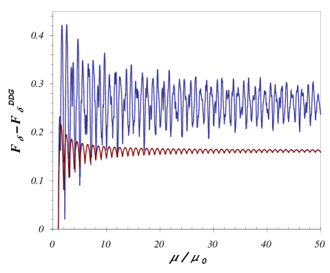
FIG. 1.: Numerical difference among the logarithmic ($F_{\delta}$) and power law ($F_{\delta}^{DDG}$) expressions discussed in the main text plotted as a function of the ratio $\mu/\mu_{0}$. The upper (lower) curve corresponds to two (one) extra dimensions.

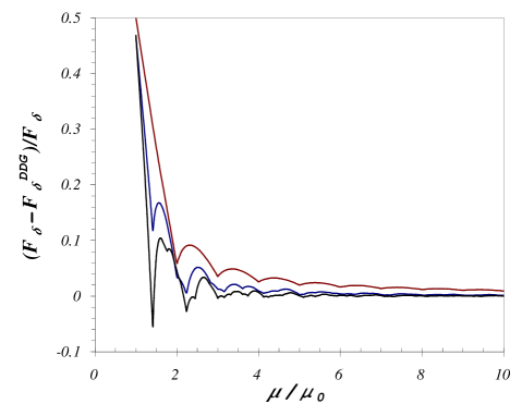
FIG. 2.: Suppression of the difference $F_{\delta}-F_{\delta}^{DDG}$ by $F_{\delta}$ displayed in terms of the ratio $\mu/\mu_{0}$. Upper (middle) curve corresponds to $\delta=1$ ($\delta=2$). The inferior curve are results for $\delta=3$.

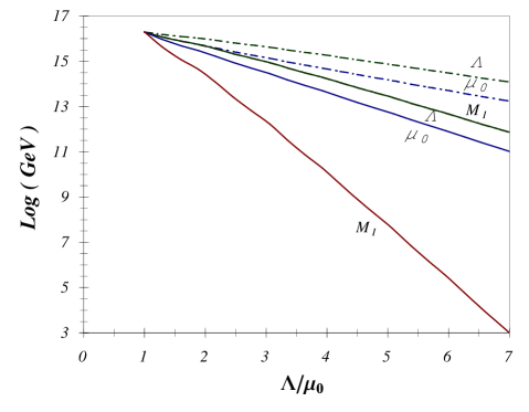
FIG. 3.: The predictions for the unification, compactification and the intermediate scales $\Lambda,\mu_{0},M_{I}$ for the case where the KK modes of the gauge bosons of the LRM are present, are plotted against of the ratio $\Lambda/\mu_{0}$. Solid (dashed) lines correspond to the case where $n_{T}=1$ and $n_{B}=2$ ($n_{B}=1$) without scalar doublets. The superposition of middle curves is an accidental effect. The extreme left corner point corresponds to the standard MSSM unification.

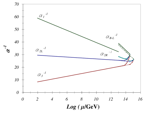
FIG. 4.: Running of the gauge couplings in the minimal (solid lines): $n_{T}=n_{B}=1$ and next to minimal (dashed lines): $n_{T}=1$; $n_{B}=2$; left right models with $M_{W_{R}}=10^{13}$ GeV; assuming that only the gauge bosons develope KK modes.

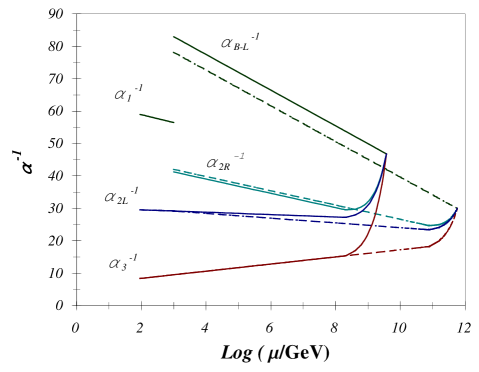
FIG. 5.: Running of the gauge couplings in the minimal (solid lines) and next to minimal (dashed lines) left right models for $M_{W_{R}}=1$ TeV; assuming that only the gauge bosons propagate into the bulk.

REFERENCES

- [1] I. Antoniadis, Phys. Lett. B246 (1990) 377; I. Antoniadis, K. Benakli and M. Quirós, Phys. Lett. B331 (1994) 313.
- [2] N. Arkani-Hamed, S. Dimopoulos and G. Dvali, Phys. Lett. B429 (1998) 263
- [3] See for example the recent discussions in: I. Antoniadis, S. Dimopoulos, G. Dvali, Nucl.Phys. B516 (1998) 70; N. Arkani-Hamed, S. Dimopoulos and G. Dvali, Phys. Rev. DD59 (1999) 086004; K. Benakli, hep-ph/9809582; Phys. Lett. B447 (1999) 51; P.Nath and M. Yamaguchi, hep-ph/9903298; hep-ph/9902323; M. L. Graesser, hep-ph/9902310. M. Masip and A. Pomarol, hep-ph/9902467; G Dvali and A.Yu. Smirnov, hep-ph/9904211.
- [4] T. Banks, A. Nelson and M. Dine, JHEP 9906 (1999) 014.
- [5] K.R. Dienes, E. Dudas and T. Gherghetta, Phys. Lett. B436 (1998) 55.
- [6] K.R. Dienes, E. Dudas and T. Gherghetta, Nucl. Phys. B537 (1999) 47.
- [7] D. Ghilencea and G.G. Ross, Phys. Lett. B442 (1998) 165.
- [8] Z. Kakushadze, Nucl. Phys. B548 (1999) 205.
- [9] C.D. Carone, Phys. Lett. B454 (1999) 70.
- [10] A. Delgado and M. Quirós, hep-ph/9903400.
- [11] P. H. Frampton and A. Rǎsin, hep-ph/9903479
- [12] G. Giudice, R. Rattazzi and J. Wells, Nucl. Phys. B544 (1999) 3; E. Mirabelli, M. Perelstein and M. Peskin, Phys. Rev. Lett.82 (1999) 2236; T. Han, J. Lykken and R. J. Zhang, Phys. Rev. D59 (1999) 105006; J. L. Hewett, Phys. Rev. Lett.82 (1999) 4765; P. Mathew, K. Sridhar and S. Raichoudhuri, Phys. Lett. B450S (1999) 343; T. G. Rizzo, Phys. Rev. D59 (1999) 115010; K. Aghase and N. G. Deshpande, hep-ph/9902263; K. Cheung and W. Y. Keung, hep-ph/9903294.
- [13] J. Lykken, Phys. Rev. D54 (1996) 3693.
- [14] T. Taylor and G. Veneziano, Phys. Lett. B212 (1988) 147.
- [15] K. Benakli, Ref. [3]; C. Burgess, L. Ibañez and F. Quevedo, Phys. Lett. B447 (1999) 257.
- [16] T. Appelquist and J. Carazzone, Phys. Rev. D11 (1975) 2856.
- [17] For a review see: A.Y. Smirnov, hep-ph/9901208 and references therein.
- [18] M. Gell-Mann, P. Rammond and R. Slansky, in Supergravity, eds. D. Freedman et al. (North-Holland, Amsterdam, 1980); T. Yanaguida, in proc. KEK workshop, 1979 (unpublished); R.N. Mohapatra and G. Senjanović, Phys. Rev. Lett.44 (1980) 912.
- [19] B. Brahmachari and R.N. Mohapatra, Int. J. of Mod. Phys. A. 10 (1996) 1699.
- [20] Particle data Group: C. Caso et al, The Europhysics Journal C3 Nos. 1-4 (1998) 1.
- [21] A. Pérez-Lorenzana, W.A. Ponce and A. Zepeda, Europhysics Lett. 39 (1997) 141; Mod. Phys. Lett. A 13 (1998) 2153.
- [22] SU(5): H.Georgi and S.L.Glashow, Phys. Rev. Lett.32 (1974) 438; H.Georgi, H.R.Quinn, and S. Weinberg, Phys. Rev. Lett.33 (1974) 451. SO(10): H.Georgi, in Particles and Fields-1974, edited by C.E.Carlson (American Institute of Physics, N.Y. 1975), p. 575; H. Fritzsch and P. Minkowski, Ann. Phys. 93 (1975) 193. E6: F.Gürsey, P.Ramond and P.Sikivie, Phys. Lett. B60 (1975) 177; S.Okubo, Phys. Rev. D16 (1977) 3528. [SU(3)]3: A. de Rújula, H.Georgi, and S. Glashow, in Fifth Workshop on Grand Unification, edited by K.Kang, H.Fried, and P.Frampton (World Scientific, Singapore, 1984), p. 88; K.S.Babu, X-G. He, and S. Pakvasa, Phys. Rev. D33 (1986) 763. SU(5) SU(5): A.Davidson and K.C.Wali, Phys. Rev. Lett.58 (1987) 2623. R.N.Mohapatra, Phys. Lett. B379 (1996) 115. SO(10) SO(10): P.Cho, Phys. Rev. D48 (1993) 5331. [SU(3)]4: This is a chiral color version of the trinification model, A. Pérez-Lorenzana and W.A. Ponce, hep-ph/9812402. [SU(4)]3: P.Cho, Phys. Rev. D48 (1993) 5331. [SU(6)]3: A.H-Galeana, R.Martínez, W.A.Ponce, and A.Zepeda, Phys. Rev. D44 (1991) 2166; W.A.Ponce and A.Zepeda, Phys. Rev. D44 (1991) 2166. [SU(6)]4: W.A. Ponce and A. Zepeda, Z.Phys. C63 (1994) 339; A. Pérez-Lorenzana, W.A. Ponce and A. Zepeda, Rev. Mex. Fis. 43 (1997) 737. For an extended discusion on different unified models see: P. Langacker, Phys.Rept. 72 (1981) 185.
- [23] J.C.Pati and A.Salam, Nucl. Phys. B50 (1979) 76; P.H.Frampton and S.L.Glashow, Phys. Lett. B190 (1987) 157.
- [24] This is a conventional normalization. Actually, represents the number of doublets in the fundamental representation of . For instance the actual values for SO(10) are . The extra factor is then absorved into the unified coupling .
- [25] J.C.Pati and A.Salam, Phys. Rev. Lett. 31 (1973) 661; V.Elias and S.Rajpoot, Phys. Rev. D20 (1979) 2445.
- [26] J.C.Pati and A.Salam, Phys. Rev. D10 (1974) 275; R.N.Mohapatra and J.C.Pati, Phys. Rev. D11 (1974) 566; D11 (1974) 2558; G. Senjanović and R.N.Mohapatra, Phys. Rev. D12 (1975) 1502.
- [27] A recent analysis for unification in the non supersymmetric left right model with non canonical embeddings was presented in A. Pérez-Lorenzana, W.A. Ponce and A. Zepeda, hep-ph/9812401; Phys. Rev. D59 (1999) 116004. See also: M. Lindner, and M. Weiser, Phys. Lett. B383 (1996) 405; D. Chang, R. N. Mohapatra, R. E. Marshak, M. Parida and J. Gipson, Phys. Rev. D31 (1985) 1718.
- [28] For a current discusion of this model see: R. Kuchimanchi and R. N. Mohapatra, Phys. Rev. D48 (1993) 4352; Phys. Rev. Lett.75 (1995) 3989; C. Aulakh, A. Melfo and G. Senjanović, Phys. Rev. D57 (1998) 4174; Z. Chacko and R. N. Mohapatra, Phys. Rev. D58 (1998) 015001; C. Aulakh, K. Benakli and G. Senjanović, Phys. Rev. Lett.79 (1997) 2188. C. S. Aulakh, A. Melfo, A. Rašin and G. Senjanović, Phys. Rev. D58 (1998) 115007; B. Dutta and R. N. Mohapatra, Phys. Rev. D 59 (1999) 015018.
- [29] K. S. Babu, C. Kolda and J. March-Russel, Euro. Phys. Journ. 3 (1998) 251.
- [30] Super-Kamiokande collaboration; ICRR-Report-419-98-15; UMD-PP-98-118.