TTP 99–19

hep-ph/9904475

28.4.99

Comparing $B\to X_{u}\ell\bar{\nu}_{\ell}$ to $B\to X_{s}\gamma$
and the Determination of $|V_{ub}|/|V_{ts}|$

Thomas Mannel and Stefan Recksiegel

Institut für Theoretische Teilchenphysik, D – 76128 Karlsruhe, Germany.

We suggest a method to determine $V_{ub}/V_{ts}$ through a comparison of $B\to X_{u}\ell\bar{\nu}_{\ell}$ and $B\to X_{s}\gamma$. The relevant quantity is the spectrum of the light-cone component of the final state hadronic momentum, which in $B\to X_{s}\gamma$ is the photon energy while in $B\to X_{u}\ell\bar{\nu}_{\ell}$ this requires a measurement of both hadronic energy and hadronic invariant mass. The non-perturbative contributions at tree level to these distributions are identical and may be cancelled by taking the ratio of the spectra. Radiative corrections to this comparison are discussed to order $\alpha_{s}$ and are combined with the non-perturbative contributions.

1 Introduction

$B$ meson decays with non-charmed final states will play an important role in the detailed investigations at future $B$–factories. Among these processes the ones involving the quark transitions $b\to u\ell\bar{\nu}_{\ell}$ and $b\to s\gamma$ are of interest with respect to the determination of $V_{ub}$ and $V_{ts}$ as well as to discover or constrain effects of physics beyond the Standard Model (SM).

From the theoretical side a lot of progress has been made by employing an expansion in inverse powers of the heavy quark mass $m_{b}$. Using operator product expansion (OPE) and the symmetries of Heavy Quark Effective Theory (HQET) [1] the nonperturbative uncertainties can be reduced to a large extent in inclusive decays [2]. Concerning the transitions mentioned above the inclusive semileptonic or radiative processes such as $B\to X_{u}\ell\bar{\nu}_{\ell}$ and $B\to X_{s}\gamma$ are the ones which we shall address in the present paper.

Looking at decay spectra of the leptons and photons in these processes, it has been pointed out that in certain regions of phase space (such as the endpoint region of the lepton energy spectrum in $B\to X_{u}\ell\bar{\nu}_{\ell}$ or the photon energy spectrum in $B\to X_{s}\gamma$ close to the endpoint of maximal energy) the correct description requires more than the naive $1/m_{b}$ expansion [3, 4, 5]. In these endpoint regions it is required to sum the leading twist contributions into a non-perturbative “shape” function, which describes the distribution of the light-cone component of the $b$ quark residual momentum inside the $B$ meson.

Unfortunately, there is no way to avoid these endpoint regions due to experimental cuts. In $B\to X_{u}\ell\bar{\nu}_{\ell}$ cuts on the lepton energy and/or on the hadronic invariant mass of the final state are required to suppress the much larger charm contribution [6, 7, 8]. Likewise, in $B\to X_{s}\gamma$ a cut on the photon energy is mandatory to reduce the background from ordinary bremsstrahlung in inclusive $B$ decays [9]. These cuts more or less reduce the accessible part of phase space to the endpoint regions. Hence it is unavoidable to get a theoretical handle on this light-cone distribution function.

The distribution function is universal, since it depends only on the properties of the initial-state $B$ hadron. This fact may be used to establish a model independent relation between the two inclusive decays $B\to X_{u}\ell\bar{\nu}_{\ell}$ and $B\to X_{s}\gamma$ [10]. Parametrizations of this function have been proposed, which include the known features such as the few lowest moments [6, 5]. It has also been shown that the popular ACCMM model [11] for a certain range of its parameters is indeed consistent with this QCD based approach [12].

There have been various suggestions how to overcome the non-perturbative uncertainties induced by the distribution function. One way is to consider moments of appropriate distributions [3, 4, 5, 13, 14]. The first few moments are then sensitive only to the first few moments of the distribution function which are known. However, due to experimental cuts only parts of the distributions can be measured such that only moments involving cuts can be obtained. Depending on the cut, these quantities are sensitive to large moments of the distribution function and in this way the non-perturbative uncertainties reappear.

In the present paper we propose a different approach. We suggest to directly compare the light-cone spectra of the final state hadrons in $B\to X_{u}\ell\bar{\nu}_{\ell}$ and $B\to X_{s}\gamma$. The individual rates depend on the shape function while the ratio of the two spectra is not very sensitive to non-perturbative effects even if cuts are included. We discuss the kinematic variables which allow a direct comparison of the two processes and consider the radiative corrections entering their relation.

In the next section we give a derivation of the non-perturbative light cone distribution. Based on this we calculate in section 3 the perturbative corrections and combine these with the non-perturbative light cone distribution function. Finally we study the comparison between $B\to X_{u}\ell\bar{\nu}_{\ell}$ and $B\to X_{s}\gamma$ quantitatively and conclude.

2 Non-perturbative Contributions: Light cone distribution function of the heavy quark

Although the derivation of how the light-cone distribution function emerges in the heavy-to-light transitions at hand is well known [3, 5, 4], we consider it useful to rederive it here, since our discussion of radiative corrections will be based on this derivation. We are going to consider heavy to light transitions such as $b\to u$ and $b\to s$ decays. The relevant effective Hamiltonian is obtained from the Standard Model by integrating out the top quark and the weak bosons. The dominant QCD corrections are taken into account as usual by running this effective interaction down to the scale of the bottom quark. The corresponding expressions are known to next-to-leading order accuracy [15, 16, 17] and one obtains for the relevant pieces

$$H_{eff}^{\rm sl}=\frac{G_{F}}{\sqrt{2}}(\bar{b}\gamma_{\mu}(1-\gamma_{5})u)(\bar{\nu}\gamma_{\mu}(1-\gamma_{5})\ell)$$ (1)

$$H_{eff}^{rare}=\frac{G_{F}}{\sqrt{2}}\frac{e}{8\pi^{2}}C_{7}(\mu)m_{b}(\mu)(\bar{b}\sigma_{\mu\nu}(1-\gamma_{5})s)|_{\mu}F^{\mu\nu}$$ (2)

mediating semileptonic $b\to u$ transitions and radiative $b\to s$ decays respectively. $C_{7}(\mu)$ is a Wilson coefficient, depending on the renormalization scale $\mu$, and $F^{\mu\nu}$ is the electromagnetic field strength.

In the following we shall consider only these two contributions; at next-to-leading order (which is the accuracy we need here) there are also contributions of other operators in the effective Hamiltonian. However, these contributions are small and can be neglected here [14], although they should be included when analyzing experimental data.

Considering the inclusive $B$ decays mediated by these two effective interactions, we shall look at the generic quantity

$$R=\sum_{X}(2\pi)^{4}\delta^{4}(p_{B}-p_{X}-q)\langle B(p_{B})|\bar{b}\Gamma q|X(p_{X})\rangle\langle X(p_{X})|\bar{q}\Gamma^{\dagger}b|B(p_{B})\rangle$$ (3)

where $q$ is the momentum transferred to the non-hadronic system and $\Gamma$ is either $\gamma_{\mu}(1-\gamma_{5})$ or $\sigma_{\mu\nu}$.

We first redefine the phase of the heavy quark field

$$b(x)=\exp(-im_{b}v\cdot x)b_{v}(x)$$ (4)

where $v$ is the velocity of the decaying $B$ meson

$$v=\frac{p_{B}}{M_{B}}\,;$$ (5)

this corresponds to a splitting of the $b$ quark momentum according to $p_{b}=m_{b}v+k$, where $k$ is a small residual momentum. Going through the usual steps, we can rewrite $R$ as

$$R=\int d^{4}x\exp(-ix[m_{b}v-q])\langle B(p_{B})|\bar{b}_{v}(0)\Gamma q(0)\bar{q}(x)\Gamma^{\dagger}b_{v}(x)|B(p_{B})\rangle$$ (6)

The momentum $P=m_{b}v-q$ is the momentum of the final state partons, which is considered to be large compared to to any of the scales appearing in the matrix element. This allows us to set up an operator product expansion (OPE). If we assume

$$(m_{b}v-q)^{2}={\cal O}(m^{2})\mbox{ and }(m_{b}-vq)={\cal O}(m)$$ (7)

the OPE is a short distance expansion yielding the usual $1/m_{b}$ expansion of the rates.

Close to the endpoint, where $P=m_{b}v-q$ is a practically light-like vector, which has still large components, i.e.

$$(m_{b}v-q)^{2}={\cal O}(\Lambda_{QCD}m_{b})\mbox{ and }(m_{b}-vq)={\cal O}(m_{b})$$ (8)

one has to switch to a light cone expansion very similar to what is known in deep inelastic scattering.

In order to study the latter case in some more detail, it is useful to define light-cone vectors as

$$n_{\pm}=\frac{1}{\sqrt{(vP)^{2}-P^{2}}}\left[v\left(\sqrt{(vP)^{2}-P^{2}}\mp(vP)\right)\pm P\right]\quad n_{\pm}^{2}=0$$ (9)

which satisfy the relations $n_{+}n_{-}=2$, $vn_{\pm}=1$ and $2v=n_{+}+n_{-}$. These vectors allow us to write

$$P=\frac{1}{2}(P_{+}n_{-}+P_{-}n_{+})\qquad P_{\pm}=Pn_{\pm}$$ (10)

where

$$P_{+}=(vP)-\sqrt{(vP)^{2}-P^{2}}\to-\frac{P^{2}}{2(vP)}\mbox{ for }P^{2}\ll(vP)^{2}$$ (11)

$$P_{-}=(vP)+\sqrt{(vP)^{2}-P^{2}}\to 2(vP)\mbox{ for }P^{2}\ll(vP)^{2}$$ (12)

The kinematic region in which the light cone distribution function becomes relevant is the one where $P_{+}$ is much smaller than $P_{-}$: Here the main contributions to the integral come from the light cone $x^{2}\approx 0$, since in order to have a contribution to the integral we need to have

$$x\cdot P=\frac{1}{2}(x_{-}P_{+}+x_{+}P_{-})=x_{+}(vP)+\mbox{ const}<\infty$$ (13)

in the limit in which $P_{-}\to\infty$. Hence $x_{+}$ has to be small, restricting the integration to the light cone.

We consider first the tree level contribution, which corresponds to a contraction of the light quark line; we get [5]

$$R = \int d^{4}x\int\frac{d^{4}Q}{(2\pi)^{4}}\Theta(Q_{0})(2\pi)\delta(Q^{2})\exp(-ix[m_{b}v-q-Q])$$ (23)

$$\langle B(v)|\bar{b}_{v}(0)\Gamma\mathchoice{\ooalign{$\hfil\displaystyle\mkern 0.0mu/\hfil$\crcr$\displaystyle Q$}}{\ooalign{$\hfil\textstyle\mkern 0.0mu/\hfil$\crcr$\textstyle Q$}}{\ooalign{$\hfil\scriptstyle\mkern 0.0mu/\hfil$\crcr$\scriptstyle Q$}}{\ooalign{$\hfil\scriptscriptstyle\mkern 0.0mu/\hfil$\crcr$\scriptscriptstyle Q$}}\Gamma^{\dagger}b_{v}(x)|B(v)\rangle$$

where now $|B(v)\rangle$ is the static $B$ meson state. Performing a (gauge covariant) Taylor expansion of the remaining $x$ dependence of the matrix element, we get

$$R = \int d^{4}x\int\frac{d^{4}Q}{(2\pi)^{4}}\Theta(Q_{0})(2\pi)\delta(Q^{2})\exp(-ix[m_{b}v-q-Q])$$ (42)

$$\sum_{n}\frac{1}{n!}\langle B(v)|\bar{b}_{v}(0)\Gamma\mathchoice{\ooalign{$\hfil\displaystyle\mkern 0.0mu/\hfil$\crcr$\displaystyle Q$}}{\ooalign{$\hfil\textstyle\mkern 0.0mu/\hfil$\crcr$\textstyle Q$}}{\ooalign{$\hfil\scriptstyle\mkern 0.0mu/\hfil$\crcr$\scriptstyle Q$}}{\ooalign{$\hfil\scriptscriptstyle\mkern 0.0mu/\hfil$\crcr$\scriptscriptstyle Q$}}\Gamma^{\dagger}(-ix\cdot iD)^{n}b_{v}(0)|B(v)\rangle$$

$$= \int d^{4}x\int\frac{d^{4}Q}{(2\pi)^{4}}\Theta(Q_{0})(2\pi)\delta(Q^{2})$$

$$\langle B(v)|\bar{b}_{v}(0)\Gamma\mathchoice{\ooalign{$\hfil\displaystyle\mkern 0.0mu/\hfil$\crcr$\displaystyle Q$}}{\ooalign{$\hfil\textstyle\mkern 0.0mu/\hfil$\crcr$\textstyle Q$}}{\ooalign{$\hfil\scriptstyle\mkern 0.0mu/\hfil$\crcr$\scriptstyle Q$}}{\ooalign{$\hfil\scriptscriptstyle\mkern 0.0mu/\hfil$\crcr$\scriptscriptstyle Q$}}\Gamma^{\dagger}{\cal P}\exp(-ix[m_{b}v-q-Q+iD])b_{v}(0)|B(v)\rangle$$

where the symbol ${\cal P}$ means the usual path–ordering of the exponential. Using spin symmetry and the usual representation matrices of the $0^{-}$ B meson states, the matrix element which appears in (42) becomes

$$\langle B(v)|\bar{b}_{v}(0)\Gamma\mathchoice{\ooalign{$\hfil\displaystyle\mkern 0.0mu/\hfil$\crcr$\displaystyle Q$}}{\ooalign{$\hfil\textstyle\mkern 0.0mu/\hfil$\crcr$\textstyle Q$}}{\ooalign{$\hfil\scriptstyle\mkern 0.0mu/\hfil$\crcr$\scriptstyle Q$}}{\ooalign{$\hfil\scriptscriptstyle\mkern 0.0mu/\hfil$\crcr$\scriptscriptstyle Q$}}\Gamma^{\dagger}(iD_{\mu_{1}})(iD_{\mu_{2}})\cdots(iD_{\mu_{n}})b_{v}(0)|B(v)\rangle$$ (51)

$$=\frac{M_{B}}{2}\mbox{Tr}\{\gamma_{5}(\mathchoice{\ooalign{$\hfil\displaystyle\mkern 0.0mu/\hfil$\crcr$\displaystyle v$}}{\ooalign{$\hfil\textstyle\mkern 0.0mu/\hfil$\crcr$\textstyle v$}}{\ooalign{$\hfil\scriptstyle\mkern 0.0mu/\hfil$\crcr$\scriptstyle v$}}{\ooalign{$\hfil\scriptscriptstyle\mkern 0.0mu/\hfil$\crcr$\scriptscriptstyle v$}}+1)\Gamma\mathchoice{\ooalign{$\hfil\displaystyle\mkern 0.0mu/\hfil$\crcr$\displaystyle Q$}}{\ooalign{$\hfil\textstyle\mkern 0.0mu/\hfil$\crcr$\textstyle Q$}}{\ooalign{$\hfil\scriptstyle\mkern 0.0mu/\hfil$\crcr$\scriptstyle Q$}}{\ooalign{$\hfil\scriptscriptstyle\mkern 0.0mu/\hfil$\crcr$\scriptscriptstyle Q$}}\Gamma^{\dagger}(\mathchoice{\ooalign{$\hfil\displaystyle\mkern 0.0mu/\hfil$\crcr$\displaystyle v$}}{\ooalign{$\hfil\textstyle\mkern 0.0mu/\hfil$\crcr$\textstyle v$}}{\ooalign{$\hfil\scriptstyle\mkern 0.0mu/\hfil$\crcr$\scriptstyle v$}}{\ooalign{$\hfil\scriptscriptstyle\mkern 0.0mu/\hfil$\crcr$\scriptscriptstyle v$}}+1)\gamma_{5}\}[a_{1}^{(n)}v_{\mu_{1}}v_{\mu_{2}}\cdots v_{\mu_{n}}+a_{2}^{(n)}g_{\mu_{1}\mu_{2}}v_{\mu_{3}}\cdots v_{\mu_{n}}+\cdots]$$ (76)

where the elipses denote terms with one or more $g_{\mu\nu}$’s and also antisymmetric terms and $a_{i}^{(n)}$ are non-pertrubative parameters. Contracting with $x^{\mu_{1}}x^{\mu_{2}}\cdots x^{\mu_{n}}$ all antisymmetric contributions vanish; furthermore, since the relevant kinematics restricts the $x_{\mu}$ to be on the light cone, also all the $g_{\mu\nu}$ terms are suppressed relative to the first term, which has only $v_{\mu}$’s. Hence

$$\langle B(v)|\bar{b}_{v}(0)\Gamma\mathchoice{\ooalign{$\hfil\displaystyle\mkern 0.0mu/\hfil$\crcr$\displaystyle Q$}}{\ooalign{$\hfil\textstyle\mkern 0.0mu/\hfil$\crcr$\textstyle Q$}}{\ooalign{$\hfil\scriptstyle\mkern 0.0mu/\hfil$\crcr$\scriptstyle Q$}}{\ooalign{$\hfil\scriptscriptstyle\mkern 0.0mu/\hfil$\crcr$\scriptscriptstyle Q$}}\Gamma^{\dagger}(-ix\cdot iD)^{n}b_{v}(0)|B(v)\rangle=M_{B}\mbox{Tr}\{(\mathchoice{\ooalign{$\hfil\displaystyle\mkern 0.0mu/\hfil$\crcr$\displaystyle v$}}{\ooalign{$\hfil\textstyle\mkern 0.0mu/\hfil$\crcr$\textstyle v$}}{\ooalign{$\hfil\scriptstyle\mkern 0.0mu/\hfil$\crcr$\scriptstyle v$}}{\ooalign{$\hfil\scriptscriptstyle\mkern 0.0mu/\hfil$\crcr$\scriptscriptstyle v$}}+1)\Gamma\mathchoice{\ooalign{$\hfil\displaystyle\mkern 0.0mu/\hfil$\crcr$\displaystyle Q$}}{\ooalign{$\hfil\textstyle\mkern 0.0mu/\hfil$\crcr$\textstyle Q$}}{\ooalign{$\hfil\scriptstyle\mkern 0.0mu/\hfil$\crcr$\scriptstyle Q$}}{\ooalign{$\hfil\scriptscriptstyle\mkern 0.0mu/\hfil$\crcr$\scriptscriptstyle Q$}}\Gamma^{\dagger}\}a_{1}^{(n)}(v\cdot x)^{n}$$ (77)

In this way we have made explicit that the kinematics we are studying here forces us to resum the series in $1/m_{b}$. Defining the twist $t$ of an operator ${\cal O}$ in the usual way $t=dim[{\cal O}]-\ell$, where $\ell$ is the spin of the operator, we find that the resummation corresponds to the contributions of leading twist, $t=3$. Since $x_{\mu}$ is light like, it projects out only the light cone component $D_{+}$ of the covariant derivative in (77). Hence we may write $a_{1}^{(n)}$ as

$$2M_{B}a_{1}^{(n)}=\langle B(v)|\bar{b}_{v}(iD_{+})^{n}b_{v}|B(v)\rangle$$ (78)

and one obtains as a final result

$$R = \int d^{4}x\int\frac{d^{4}Q}{(2\pi)^{4}}\Theta(Q_{0})(2\pi)\delta(Q^{2})\frac{1}{2}\mbox{Tr}\{(\mathchoice{\ooalign{$\hfil\displaystyle\mkern 0.0mu/\hfil$\crcr$\displaystyle v$}}{\ooalign{$\hfil\textstyle\mkern 0.0mu/\hfil$\crcr$\textstyle v$}}{\ooalign{$\hfil\scriptstyle\mkern 0.0mu/\hfil$\crcr$\scriptstyle v$}}{\ooalign{$\hfil\scriptscriptstyle\mkern 0.0mu/\hfil$\crcr$\scriptscriptstyle v$}}+1)\Gamma\mathchoice{\ooalign{$\hfil\displaystyle\mkern 0.0mu/\hfil$\crcr$\displaystyle Q$}}{\ooalign{$\hfil\textstyle\mkern 0.0mu/\hfil$\crcr$\textstyle Q$}}{\ooalign{$\hfil\scriptstyle\mkern 0.0mu/\hfil$\crcr$\scriptstyle Q$}}{\ooalign{$\hfil\scriptscriptstyle\mkern 0.0mu/\hfil$\crcr$\scriptscriptstyle Q$}}\Gamma^{\dagger}\}$$

$$\langle B(v)|\bar{b}_{v}\exp(-ix[(m_{b}+iD_{+})v-q-Q])b_{v}|B(v)\rangle$$

Introducing the shape function (or light cone distribution function) as [3, 5, 4]

$$2M_{B}f(k_{+})=\langle B(v)|\bar{b}_{v}\delta(k_{+}-iD_{+})b_{v}|B(v)\rangle$$ (96)

we can write the result as

$$R = \int dk_{+}f(k_{+})\int\frac{d^{4}Q}{(2\pi)^{4}}\Theta(Q_{0})(2\pi)\delta(Q^{2})$$ (114)

$$M_{B}\mbox{Tr}\{(\mathchoice{\ooalign{$\hfil\displaystyle\mkern 0.0mu/\hfil$\crcr$\displaystyle v$}}{\ooalign{$\hfil\textstyle\mkern 0.0mu/\hfil$\crcr$\textstyle v$}}{\ooalign{$\hfil\scriptstyle\mkern 0.0mu/\hfil$\crcr$\scriptstyle v$}}{\ooalign{$\hfil\scriptscriptstyle\mkern 0.0mu/\hfil$\crcr$\scriptscriptstyle v$}}+1)\Gamma\mathchoice{\ooalign{$\hfil\displaystyle\mkern 0.0mu/\hfil$\crcr$\displaystyle Q$}}{\ooalign{$\hfil\textstyle\mkern 0.0mu/\hfil$\crcr$\textstyle Q$}}{\ooalign{$\hfil\scriptstyle\mkern 0.0mu/\hfil$\crcr$\scriptstyle Q$}}{\ooalign{$\hfil\scriptscriptstyle\mkern 0.0mu/\hfil$\crcr$\scriptscriptstyle Q$}}\Gamma^{\dagger}\}(2\pi)^{4}\delta^{4}([m_{b}+k_{+}]v-Q-q)$$

This result shows that the leading twist contribution is obtained by convoluting the partonic result with the shape function, where in the partonic result the $b$ quark mass $m_{b}$ is replaced by the mass

$$m_{b}^{*}=m_{b}+k_{+}$$ (115)

Let us take a closer look at the kinematics. The final-state quark is massless,

$$0=([m_{b}+k_{+}]v-q)^{2}$$

in which case we have for the light cone component of the heavy quark residual momentum

$$k_{+}=-m_{b}+(vq)+\sqrt{(vq)^{2}-q^{2}}$$ (116)

Note that this variable – up to a minus sign – is just $P_{+}$ and thus close to the endpoint

$$k_{+}\approx-\frac{P^{2}}{2(vP)}$$ (117)

If we now look at the hadronic kinematics

$$M_{B}v-q=p_{X}\,,$$ (118)

where $p_{X}$ is the four momentum of the final state hadrons, and use the relation between the heavy quark mass and the meson mass

$$M_{B}=m_{b}+\bar{\Lambda}+{\cal O}(1/m_{b})$$ (119)

we find

$$p_{X}=P+\bar{\Lambda}v\quad\mbox{ or }\quad p_{X\pm}=P_{\pm}+\bar{\Lambda}$$ (120)

Thus the light cone component of the hadronic momentum of the final state

$$L_{+}=-p_{X+}=-M_{B}+(vq)+\sqrt{(vq)^{2}-q^{2}}$$ (121)

ranging between $-M_{B}\leq L_{+}\leq 0$ is directly related to the light-cone component of the residual momentum of the heavy quark

$$L_{+}=k_{+}-\bar{\Lambda}$$ (122)

where the range of $k_{+}$ is given by $-m_{b}\leq k_{+}\leq\bar{\Lambda}$. However, large negative values of $k_{+}$ close to $-m_{b}$ are beyond the validity of the heavy mass limit.

The observable $L_{+}$ directly measures the light cone component of the residual momentum of the heavy quark, at least for small values of $L_{+}$. In the case of $b\to s\gamma$ we have $q^{2}=0$ and $L_{+}$ is directly related to the energy $E_{\gamma}$ of the photon in the rest frame of the decaying $B$

$$L_{+}=-M_{B}+2E_{\gamma}.$$

For $b\to u\ell\bar{\nu}_{\ell}$ a reconstruction of $L_{+}$ requires both a measurement of the hadronic energy and the hadronic invariant mass.

Reexpressing the convolution (114) in terms of $L_{+}$ and using that the light-cone distribution function is non-vanishing only for $-m_{b}\to-\infty<k_{+}<\bar{\Lambda}$ we may rewrite (114) as

$$R = \int\limits_{-M_{B}}^{0}dL_{+}f(L_{+}+\bar{\Lambda})\int\frac{d^{4}Q}{(2\pi)^{4}}\Theta(Q_{0})(2\pi)\delta(Q^{2})$$ (140)

$$M_{B}\mbox{Tr}\{(\mathchoice{\ooalign{$\hfil\displaystyle\mkern 0.0mu/\hfil$\crcr$\displaystyle v$}}{\ooalign{$\hfil\textstyle\mkern 0.0mu/\hfil$\crcr$\textstyle v$}}{\ooalign{$\hfil\scriptstyle\mkern 0.0mu/\hfil$\crcr$\scriptstyle v$}}{\ooalign{$\hfil\scriptscriptstyle\mkern 0.0mu/\hfil$\crcr$\scriptscriptstyle v$}}+1)\Gamma\mathchoice{\ooalign{$\hfil\displaystyle\mkern 0.0mu/\hfil$\crcr$\displaystyle Q$}}{\ooalign{$\hfil\textstyle\mkern 0.0mu/\hfil$\crcr$\textstyle Q$}}{\ooalign{$\hfil\scriptstyle\mkern 0.0mu/\hfil$\crcr$\scriptstyle Q$}}{\ooalign{$\hfil\scriptscriptstyle\mkern 0.0mu/\hfil$\crcr$\scriptscriptstyle Q$}}\Gamma^{\dagger}\}(2\pi)^{4}\delta^{4}([M_{B}+L_{+}]v-Q-q)$$

where we have made use of (119). Equivalently, we may write the spectrum in the variable $L_{+}$ as

$$\frac{dR}{dL_{+}} = f(L_{+}+\bar{\Lambda})\int\frac{d^{4}Q}{(2\pi)^{4}}\Theta(Q_{0})(2\pi)\delta(Q^{2})$$ (158)

$$M_{B}\mbox{Tr}\{(\mathchoice{\ooalign{$\hfil\displaystyle\mkern 0.0mu/\hfil$\crcr$\displaystyle v$}}{\ooalign{$\hfil\textstyle\mkern 0.0mu/\hfil$\crcr$\textstyle v$}}{\ooalign{$\hfil\scriptstyle\mkern 0.0mu/\hfil$\crcr$\scriptstyle v$}}{\ooalign{$\hfil\scriptscriptstyle\mkern 0.0mu/\hfil$\crcr$\scriptscriptstyle v$}}+1)\Gamma\mathchoice{\ooalign{$\hfil\displaystyle\mkern 0.0mu/\hfil$\crcr$\displaystyle Q$}}{\ooalign{$\hfil\textstyle\mkern 0.0mu/\hfil$\crcr$\textstyle Q$}}{\ooalign{$\hfil\scriptstyle\mkern 0.0mu/\hfil$\crcr$\scriptstyle Q$}}{\ooalign{$\hfil\scriptscriptstyle\mkern 0.0mu/\hfil$\crcr$\scriptscriptstyle Q$}}\Gamma^{\dagger}\}(2\pi)^{4}\delta^{4}([M_{B}+L_{+}]v-Q-q)$$

The two relations (140) and (158) exhibit an interesting feature of the summation of the leading twist terms, namely that the dependence on the heavy quark mass has completely disappeared, only the shape function $f$ still depends on $\bar{\Lambda}$. The full result should be independent of this unphysical quantity and hence the explicit dependence on $\bar{\Lambda}$ of the shape function has to cancel against the one appearing in the argument of the shape function. In other words, if we write the shape function as $f=f(k_{+},\bar{\Lambda})$, this function of two variables has to satisfy

$$\left(\frac{\partial}{\partial k_{+}}+\frac{\partial}{\partial\bar{\Lambda}}\right)f(k_{+},\bar{\Lambda})=0\quad\mbox{ or }\quad f(k_{+},\bar{\Lambda})=g(k_{+}-\bar{\Lambda})$$ (159)

In this way the total result becomes independent of any reference to the quark mass $m_{b}$ or equivalently on $\bar{\Lambda}$. In particular, (159) ensures the cancellation of ambiguities related to the renormalon in the heavy quark mass [12].

Putting everything together, the light-cone spectrum (158) for the decay $B\to X_{u}\ell\bar{\nu}_{\ell}$ becomes

$$\frac{d\Gamma}{dL_{+}}(B\to X_{u}\ell\bar{\nu}_{\ell})=\frac{G_{F}^{2}(M_{B}+L_{+})^{5}|V_{ub}|^{2}}{192\pi^{3}}g(L_{+})$$ (160)

which means that the spectrum is proportional to the total rate in which the $m_{b}$ has been replaced by $M_{B}+K_{+}$.

Similarly, for $B\to X_{s}\gamma$ one finds

$$\frac{d\Gamma}{dL_{+}}(B\to X_{s}\gamma)=\frac{G_{F}^{2}(M_{B}+L_{+})^{5}|V_{tb}V_{ts}^{*}|^{2}\alpha_{em}}{32\pi^{4}}[C_{7}(M_{B})]^{2}g(L_{+})$$ (161)

Note that (160) and (161) do not depend on any unphysical parameter, since the $\bar{\Lambda}$ dependence has disappeared. In particular, all ambiguities induced by renormalons should cancel in these equations. Based on this it has been suggested to give a definition for a heavy quark mass $\hat{m}_{b}$ through (160) and (161) using e.g. the mean energy $\langle E_{\gamma}\rangle$ of the photon in $B\to X_{s}\gamma$ [13]. To this end we consider the moments of the function $g$, which can be obtained from the moments of the shape function $f$. The usual HQET relations are

$$\int_{-\infty}^{\bar{\Lambda}}dk_{+}f(k_{+})=1$$ (162)

$$\int_{-\infty}^{\bar{\Lambda}}dk_{+}k_{+}f(k_{+})=\delta m_{b}$$ (163)

$$\int_{-\infty}^{\bar{\Lambda}}dk_{+}k_{+}^{2}f(k_{+})=-\frac{1}{3}\lambda_{1}$$ (164)

which define the normalization, the residual mass term [18] and the kinetic energy parameter.

Reexpressing relation (163) through the function $g$ we have

$$\int_{-\infty}^{0}dL_{+}L_{+}g(L_{+})=\delta m_{b}-\bar{\Lambda}\equiv\hat{\Lambda}$$ (165)

which gives a definition of the heavy quark mass $\hat{m_{b}}=M_{B}-\hat{\Lambda}$ free of renomalon ambiguities which cancel between the $\delta m_{b}$ and $\bar{\Lambda}$ [13].

For the second moment one obtains from (164)

$$\int_{-\infty}^{0}dL_{+}L_{+}^{2}g(L_{+})=-\frac{1}{3}\lambda_{1}-\bar{\Lambda}^{2}-2\bar{\Lambda}\hat{\Lambda}\equiv-\frac{1}{3}\hat{\lambda}_{1}$$ (166)

where $\hat{\lambda}_{1}$ again has to be free of renormalon ambiguities.

We shall later need a model shape function to discuss our results. In order to keep things simple, we use the one-parameter model of [5]

$$g(L_{+}) = {32\over\pi^{2}\sigma^{3}}L_{+}^{2}\exp\left[-{4\over\pi\sigma^{2}}L_{+}^{2}\right]\Theta(-L_{+})$$ (167)

which is easy to deal with. Here $\sigma$ is the width parameter of the shape function and will be varied in our numerical studies between 400 MeV and 800 MeV.

3 Including Perturbative Contributions

The next step is to include radiative corrections to the relations (160) and (161). The starting point of the considerations is (114) or eqivalently (140). However, now the partonic result $d\Gamma_{part}$ including the radiative corrections is convoluted with the shape function

$$d\Gamma_{had}=\int\limits_{-m_{b}}^{\bar{\Lambda}}d\Gamma_{part}(m_{b}^{*}=m_{b}+k_{+})f(k_{+})dk_{+}$$ (168)

We shall compute the spectrum in the light cone variable of the hadronic momentum $L_{+}$, and the partonic counterpart of this variable is

$$l_{+}=-m_{b}+(vq)+\sqrt{(vq)^{2}-q^{2}}\,.$$ (169)

in which we compute a differential spectrum as some function $G$ of $l_{+}$ and $m_{b}$

$$\frac{d\Gamma_{part}}{dl_{+}}=G(m_{b},l_{+})\,.$$ (170)

To apply the convolution formulae (114) and (140) we replace in the first step the heavy quark mass by $m_{b}^{*}$ and convolute with the shape function. The variable $l_{+}$ is also replaced by

$$l_{+}^{*}=-m_{b}^{*}+(vq)+\sqrt{(vq)^{2}-q^{2}}=l_{+}-k_{+}$$ (171)

Note that $l_{+}^{*}$ is again a light cone variable for a process in which the heavy quark mass is replaced by $m_{b}^{*}$, and hence it ranges between $-m_{b}^{*}\leq l_{+}^{*}\leq 0$, which means that the $k_{+}$ integration becomes restricted to

$$-l_{+}\leq k_{+}\leq\bar{\Lambda}$$ (172)

The second step towards hadronic variables is to replace $l_{+}$ by $L_{+}$, the hadronic light cone momentum. At the same time we perform a shift in the integration variable $k_{+}\to K_{+}-\bar{\Lambda}$ and obtain

$$\frac{d\Gamma_{had}}{dL_{+}}=\int\limits_{L_{+}}^{0}dK_{+}\,G(M_{B}+K_{+},L_{+}-K_{+})g(K_{+})$$ (173)

Relation (173) holds for any $b\to q$ transition where $q$ is a light quark. We shall exploit (173) for a comparison between the inclusive processes $B\to X_{s}\gamma$ and $B\to X_{u}\ell\bar{\nu}_{\ell}$. The partonic $l_{+}$ spectra of the two processes can be calculated; both take the generic form

$$G(m_{b},l_{+}) = \gamma_{0}m_{b}^{5}\left[(1+b_{0}\frac{\alpha_{s}}{3\pi})\delta(l_{+})+\vphantom{\int\limits_{t}^{t}}\right.$$

$$\left.\frac{\alpha_{s}}{3\pi}\left(b_{1}\left(\frac{\ln(-l_{+}/m_{b})}{-l_{+}}\right)_{+}+b_{2}\left(\frac{1}{-l_{+}}\right)_{+}+\frac{1}{m_{b}}\Phi\left(\frac{-l_{+}}{m_{b}}\right)\right)\right]$$

where we have defined the “+”-distributions in the usual way

$$\int_{0}^{1}dxD_{+}(x)=0\,,$$ (175)

and $b_{0}$, $b_{1}$, $b_{2}$ and $\Phi$ are known quantities. For $b\to u\ell\bar{\nu}_{\ell}$ we find

$$\gamma_{0} = {G_{F}^{2}\left|V_{ub}\right|^{2}\over 192\pi^{3}}$$ (176)

$$b_{0} = -{13\over 36}-2\pi^{2}$$

$$b_{1} = -4$$

$$b_{2} = -26/3$$

$$\Phi(x) = \frac{158}{9}+\frac{407\,x}{18}-\frac{367\,{x^{2}}}{6}+\frac{118\,{x^{3}}}{3}-\frac{100\,{x^{4}}}{9}+\frac{11\,{x^{5}}}{6}-\frac{7\,{x^{6}}}{18}$$

$$-\frac{4\,\ln(x)}{3}+\frac{46\,x\,\ln(x)}{3}+6\,{x^{2}}\,\ln(x)-\frac{16\,{x^{3}}\,\ln(x)}{3}$$

$$-12\,{x^{2}}\,{{\ln(x)}^{2}}+8\,{x^{3}}\,{{\ln(x)}^{2}}$$

While for $b\to s\gamma$

$$\gamma_{0} = {G_{F}^{2}\left|V_{ts}V_{tb}^{*}\right|^{2}\left|C_{7}\right|^{2}\alpha_{\rm em}\over 32\pi^{4}}$$ (177)

$$b_{0} = -5-\frac{4}{3}\pi^{2}$$

$$b_{1} = -4$$

$$b_{2} = -7$$

$$\Phi(x) = 6+3\,x-2\,{x^{2}}-4\,\ln(x)+2\,x\,\ln(x)$$

where $C_{7}=-0.306$ is obtained from the next-to-leading order calculation of [17]. Our result for $B\to X_{s}\gamma$ coincides with the ones obtained in the literature [16, 17, 19]. To determine $b_{0}$ for $B\to X_{u}\ell\bar{\nu}_{\ell}$ and $B\to X_{s}\gamma$ the respective total rates at ${\cal O}(\alpha_{s})$ [20, 21] have been used.

The partonic result up to order $\alpha_{s}$ contains terms of all orders in the $1/m_{b}$ expansion and we shall first consider the leading twist contribution. Taking the limit $m_{b}\to\infty$ of the partonic calculation leaves us only with the “+”-distributions and the $\delta$ function. The convolution becomes

$$\frac{d\Gamma_{had}}{dL_{+}} = \int\limits_{L_{+}}^{0}dK_{+}\,g(K_{+})\gamma_{0}(M_{B}+K_{+})^{5}\left[(1+b_{0}\frac{\alpha_{s}}{3\pi})\delta(L_{+}-K_{+})\vphantom{\int\limits_{t}^{t}}\right.$$

$$+\frac{\alpha_{s}}{3\pi}\left.\left(b_{1}\left(\frac{\ln\left(\frac{-L_{+}+K_{+}}{M_{B}+K_{+}}\right)}{-L_{+}+K_{+}}\right)_{+}+b_{2}\left(\frac{1}{-L_{+}+K_{+}}\right)_{+}\right)\right]$$

The shape function $g(K_{+})$ is restricted to values $K_{+}$ small compared to $M_{B}$, and one may expand the dependence on $M_{B}+K_{+}$ for small $K_{+}$. This induces terms of higher orders in $1/m_{b}$, which again may be dropped. Hence the leading twist terms become

$$\frac{d\Gamma_{had}}{dL_{+}} = \gamma_{0}M_{B}^{5}\left[(1+b_{0}\frac{\alpha_{s}}{3\pi})g(L_{+})+\vphantom{\int\limits_{t}^{t}}\right.$$

$$\left.\frac{\alpha_{s}}{3\pi}\int\limits_{L_{+}}^{0}dK_{+}g(K_{+})\left(b_{1}\left(\frac{\ln\left(\frac{-L_{+}+K_{+}}{M_{B}}\right)}{-L_{+}+K_{+}}\right)_{+}+b_{2}\left(\frac{1}{-L_{+}+K_{+}}\right)_{+}\right)\right]$$

It is well known that the coefficient $b_{1}$ is universal as well as the shape function. This suggests to define a scale dependent shape function, which to order $\alpha_{s}$ becomes

$${\cal F}(K_{+},\mu)=g(K_{+})+\frac{\alpha_{s}b_{1}}{3\pi}\int\limits_{L_{+}}^{0}dK_{+}g(K_{+})\left(\frac{\ln\left(\frac{-L_{+}+K_{+}}{\mu}\right)}{-L_{+}+K_{+}}\right)_{+}$$ (180)

The scale dependence of the distribution function has been discussed in [22], where the evolution equation for the distribution function has been set up.

The terms proportional to $(1/l_{+})_{+}$ are not universal, which is natural, since the relavant scale in two different processes may be different. A change of scale changes the contribution of the $(\alpha_{s}/\pi)(1/l_{+})_{+}$ pieces according to

$${\cal F}(K_{+},\mu)={\cal F}(K_{+},\mu^{\prime})+\frac{\alpha_{s}b_{1}}{3\pi}\int\limits_{L_{+}}^{0}dK_{+}g(K_{+})\ln\left(\frac{\mu^{\prime}}{\mu}\right)\left(\frac{1}{-L_{+}+K_{+}}\right)_{+}$$ (181)

and hence we find for the leading twist contribution

$$\frac{d\Gamma_{had}}{dL_{+}}=\gamma_{0}M_{B}^{5}(1+b_{0}\frac{\alpha_{s}}{3\pi}){\cal F}(L_{+},\mu)$$ (182)

where the scale $\mu$ is given by

$$\ln\left(\frac{M_{B}}{\mu}\right)=\frac{b_{2}}{b_{1}}$$ (183)

Inserting the results for the two processes under consideration we find

$$\mu_{b\to s\gamma}=0.1738M_{b}\qquad\mu_{b\to u\ell\bar{\nu}_{\ell}}=0.1146M_{b}$$ (184)

which are in fact scales small compared to the mass of the $b$ quark. Furthermore, the ratio of the two scale is of order one,

$$\frac{\mu_{b\to s\gamma}}{\mu_{b\to u\ell\bar{\nu}_{\ell}}}\approx 1.52$$ (185)

The physical meaning of the scale $\mu$ can be understood in a picture as proposed in [23]. Here the amplitude is decomposed into a hard part, a “jetlike” part incorporating the collinear singularities and a soft part. The typical scales corresponding to these pieces are $m_{b}^{2}$ for the hard, $\Lambda_{QCD}m_{b}$ for the “jetlike” and $\Lambda_{QCD}^{2}$ for the soft part. Comparing the present approach to [23] the light-cone distribution function corresponds to the convolution of the soft and the “jetlike” piece, both of which are universal but scale dependent.

Thus the scale appearing in the shape function should be of the order $\mu^{2}\sim m_{b}\Lambda_{QCD}$ since it incorporates all lower scales. In particular, the shape function combines both the collinear and the soft contributions which according to [23] could be factorized. Since we are working to next–to–leading order, we can fix the scale according to (183), and we expect to obtain a scale $\mu^{2}$ of order $\Lambda_{QCD}m_{b}\sim 0.9$ GeV², which is confirmed by (184).

The rest of the partonic result, i.e. the function $\Phi$, is a contribution of subleading terms, suppressed by at least one power of the heavy mass. We shall use these terms to estimate, how far we can trust the leading twist terms, in particular in the comparison between $B\to X_{u}\ell\bar{\nu}_{\ell}$ and $B\to X_{s}\gamma$. To this end we add the two contributions and use the expression

$$\frac{d\Gamma_{had}}{dL_{+}}=\gamma_{0}M_{B}^{5}\left[(1+b_{0}\frac{\alpha_{s}}{3\pi}){\cal F}(L_{+},\mu)+\frac{\alpha_{s}}{3\pi M_{B}}\Phi\left(-\frac{L_{+}}{M_{B}}\right)\right]$$ (186)

We note that the functions $\Phi$ for both processes contain terms diverging logarithmically as $L_{+}\to 0$, but which are suppressed by $1/m_{b}$. These divergencies will be cured once the analogon of the light-cone distribution function at subleading order is taken into account. However, for the quantitative analyis of the process these terms are not important as long as we do not get too close to the endpoint.

4 Comparison of $B\to X_{u}\ell\bar{\nu}_{\ell}$ to $B\to X_{s}\gamma$

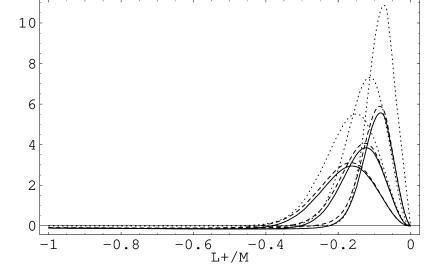
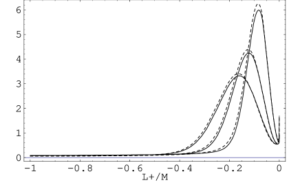
Figure 1: Light-cone distribution spectra for $B\to X_{u}\ell\bar{\nu}_{\ell}$ (solid) and $B\to X_{s}\gamma$ (dashed) in units of $\gamma_{0}M_{B}^{5}$. The dotted line is the leading contribution, which is the same for both processes. The three sets of curves correspond to values of $\sigma$ of 400, 600 and 800 MeV.

We shall first study the $L_{+}$ spectra of the two processes using (182) and (186). These results depend on the model for the shape function one is using and we shall employ the simple one-parameter model (167). In fig.1 we show the $L_{+}$ spectra of $B\to X_{u}\ell\bar{\nu}_{\ell}$ and $B\to X_{s}\gamma$. We divide the rates by the prefactors $\gamma_{0}M_{B}^{2}$, such that at leading order only the shape function remains. The left plot shows the shape function (167) together with the leading twist contribution (182) for the two processes for three different values of the width parameter $\sigma$.

The leading twist contribution can only be trusted close to the endpoint $L_{+}=0$; it even becomes negative for values $L_{+}\leq-\sigma$, indicating the breakdown of the leading twist approximation. Adding the subleading terms as in (186) cures this problem and the results are shown in the right hand figure of fig.1. The sharp rise of the full results is due to the logarithms $\ln L_{+}$ of order $1/m_{b}$, which become relevant only very close to $L_{+}=0$. These contributions are integrable and will not be relevant once the rates are binned with reasonably large bins.

Next we shall compare $B\to X_{u}\ell\bar{\nu}_{\ell}$ to $B\to X_{s}\gamma$ by considering the ratio of the two $L_{+}$ distributions. From the experimental point of view many systematic uncertainties cancel, while from the theoretical side one expects to reduce nonperturbative uncertainties, which indeed at tree level cancel completely.

The perturbative result for the spectrum is a distribution and the ratio of the perturbative expressions is meaningless, even if we avoid the region around $L_{+}=0$. However, once we have combined both perturbative and non-perturbative contributions we can take the ratio without encountering the problem of distributions.

The price we have to pay is that the resulting ratio is not independent of the shape function, an effect which has been observed already in [10]. Still the ratio of the two processes is a useful quantity, since one may expect that much of the non-perturbative uncertainties still cancel.

Figure 2: Ratio of the light cone distribution spectra for the two processes. The leading twist contribution (187) is given in the left plot while the right plot shows the full result. The solid, dashed and dotted lines correspond to values of $\sigma$ of 600, 400 and 800 MeV, respectively.

The two spectra are due to the “smearing” with the nonperturbative shape function smooth curves and we can perform a comparison of the two processes by taking the ratio. At leading twist this ratio becomes

$$\frac{(d\Gamma_{B\to X_{u}\ell\bar{\nu}_{\ell}}/dL_{+})}{(d\Gamma_{B\to X_{s}\gamma}/dL_{+})}=\frac{|V_{ub}|^{2}}{|V_{ts}V_{tb}^{*}|^{2}}\frac{\pi}{6\alpha_{em}|C_{7}|^{2}}\frac{{\cal F}(L_{+},\mu_{b\to s\ell\bar{\nu}_{\ell}})}{{\cal F}(L_{+},\mu_{b\to s\gamma})}\left(1+\frac{\alpha_{s}(m_{b})}{3\pi}\left[\frac{167}{36}-\frac{2}{3}\pi^{2}\right]\right)$$ (187)

where the scales of the distribution functions have been given in (184). It is interesting to note that although the radiative corrections at leading twist (the constants $b_{0}$) are big for the individual processes, they turn out to be small in the ratio (187).

For values of $L_{+}$ within the nonperturbative region $L_{+}\geq-\sigma$ the leading twist contribution is dominant and the comparison may be performed using the leading twist terms only. This is the region with the largest fraction of the total rate and hence the subleading terms will not play a role, also due to experimental cuts. The ratio of the leading twist terms is shown in the left hand plot of fig.2 for three values of the parameter $\bar{\Lambda}$.

The region of validity of the leading twist contribution may be studied by looking at the ratio of the full results (186) shown in fig(2). The subleading terms lead to a minimum at the point where they are becomming the dominant contribution to the rates. This happens at values of $L_{+}$ which correspond to the typical width $\sigma$ of the non-perturbative shape function.

For values of $L_{+}$ between $-\sigma$ and $0$ one may then use our results to determine CKM matrix elements, since the ratio of the two rates depends on

$$\frac{|V_{ub}|^{2}}{|V_{ts}V_{tb}^{*}|^{2}}\frac{\pi}{6\alpha_{em}|C_{7}|^{2}}\approx 5$$

i.e. the results shown in fig.2 have to be multiplied by this factor. Hence one may determine $|V_{ub}|/|V_{ts}|$ in this way; however, the radiative corrections induce a small hadronic uncertainty, which is hard to quantify without knowledge of the non-perturbative distribution function. Still one may expect only a small uncertainty, since at tree level there is no hadronic uncertainty at all.

5 Conclusions

Due to experimental constraints severe cuts on the phase space in both $b\to s\gamma$ and $b\to u\ell\bar{\nu}_{\ell}$ inclusive transitions have to be imposed making these decays sensitive to non-perturbative effects. Within the framework of the heavy mass expansion of QCD these effects are encoded in a light-cone distribution function which is universal for all heavy to light processes.

The universality of this function may be exploited to eliminate the non-perturbative uncertainties in $b\to s\gamma$ using the input of $b\to u\ell\bar{\nu}_{\ell}$ or vice versa. To this end, one may use the comparison of the two processes to determine the ratio $V_{ub}/V_{ts}$ or — for fixed CKM parameters — to test the Wilson coefficient $C_{7}$.

The comparison between the two processes is best performed in terms of the spectra of the light-cone component of the final state hadrons, which for the case of $B\to X_{s}\gamma$ is equivalent to the photon energy spectrum, while for $B\to X_{u}\ell\bar{\nu}_{\ell}$ this requires a measurement of both the hadronic invariant mass and the hadronic energy.

For small values, the light cone component of the final state hadrons is the same as the light cone component of the heavy quark residual momentum. The corresponding spectra are at tree level directly proportional to the light cone distribution function and hence one may access this function by a measurement of the the light cone distribution of the momentum of the final state hadrons.

However, radiative corrections change this picture. The main effect is that the shape function does not cancel any more in the ratio of the two spectra. The partonic radiative corrections to the light-cone distribution of the final state partons exhibit the well known singularities of the type $\ln l_{+}/l_{+}$ and $1/l_{+}$ which can be absorbed into a radiatively corrected, scale dependent light cone distribution function. It turns out that the relevant scales are small in both cases and different. The scale dependent distribution functions involve a convolution such that the nonperturbative effects cannot be cancelled anymore in the ratio.

We have also computed the subleading terms partonically and use this to estimate the reliability of the leading twist comparison of $B\to X_{s}\gamma$ and $B\to X_{u}\ell\bar{\nu}_{\ell}$. This comparison depends on the width of the non-perturbative function once radiative corrections are taken into account. For values of $L_{+}$ close to the endpoint (i.e. within the width of the distribution function) one may use the leading twist contribution to extract $|V_{ub}|/|V_{ts}|$ with reduced hadronic uncertainties. This method should become feasible at the future $B$ physics experiments.

References

[1]M.B. Voloshin and M.A. Shifman, Sov. J. Nucl. Phys. 45 (1987) 292,
Sov. J. Nucl. Phys. 47 (1988) 511;
N. Isgur and M.B. Wise, Phys. Lett. B232 (1989) 113,
Phys. Lett. B 237 (1990) 527;
E. Eichten and B. Hill, Phus. Lett. B 234 (1990) 511;
B. Grinstein, Nucl. Phys. B 339 (1990) 253;
H. Georgi, Phys. Lett B 240 (1990) 447;
A.F. Falk, H. Georgi and M.B. Wise, Nucl. Phys. B 343 (1990) 1
[2] I. Bigi, N. Uraltsev and A. Vainshtein,
Phys. Lett. B293 (1992) 430;
I. Bigi et al., Phys. Rev. Lett. 71 (1993) 496.
A. Manohar and M. Wise,
Phys. Rev. D49 (1994) 1310;
T. Mannel, Nucl. Phys. B423 (1994) 396;
for a recent review see Z. Ligeti, talk at the
DPF’99 Conference,
Jan. 5-9, 1999, Los Angeles, CA, hep-ph/9904460.
[3]M. Neubert, Phys. Rev. D49 (1994) 3392.
[4]I.I. Bigi, M.A. Shifman, N.G. Uraltsev and A.I. Vainshtein,
Int. J. Mod. Phys. A 9 (1994) 2467
[5]T. Mannel and M. Neubert, Phys. Rev. D 50
(1994) 2037.
[6]The BaBar Physics Book, Eds. H. Quinn and P.Harrison,
SLAC report 504 R (1998).
[7] I. Bigi, R.D. Dikeman, N. Uraltsev,
Eur. Phys. J. C4 (1998) 453.
[8] A. F. Falk, Z. Ligeti, M. Wise
Phys. Lett. B406 (1997) 225.
[9]M.S. Alam et al., Phys. Rev. Lett. 74 (1995) 2885
R. Barate et al., Phys. Lett. B 429 (1998) 169
[10]M. Neubert, Phys. Rev. D 49 (1994) 4623.
[11] G. Altarelli et al.,
Nucl. Phys. B208 (1982) 365.
[12] I. Bigi et al,
Phys. Lett. B 328 (1994) 431.
[13] C. Bauer, Phys. Rev. D 57 (1998) 5611.
[14] Z. Ligeti, M. Luke, A. Manohar, M. Wise
preprint FERMILAB-PUB-99-025-T, Mar 1999,
e-Print Archive: hep-ph/9903305
[15] G. Buchalla, A. Buras, M. Lautenbacher,
Rev. Mod. Phys. 68 (1996) 1125.
[16]A. Ali, C. Greub, Phys. Lett. B 361 (1995) 146.
[17]K. Chetyrkin, M. Misiak and M. Münz,
Phys. Lett. B 400 (1997) 206;
C. Greub, T. Hurth, Phys. Rev. D 56 (1997) 2934;
C. Greub, T. Hurth, D. Wyler,
Phys. Rev. D 54 (1996) 3350.
[18]A.F. Falk, M. Neubert, M. Luke, Nucl.Phys.
B 388 (1992) 363.
[19]A.L. Kagan and M. Neubert,
Eur. Phys. J. C 7 (1999) 5.
[20]T. Kinoshita and A. Sirlin, Phys. Rev. 113 (1959) 1652
S.M. Berman, Phys. Rev. 112 (1958) 267
T. van Ritbergen, hep-ph/9903226
[21]N. Pott, Phys. Rev. D 54 (1996) 938
[22]C. Balzereit, W. Kilian and T. Mannel, Phys. Rev. D 58 (1998) 114029
[23]G.P. Korchemsky, G. Sterman, Phys. Lett.
B 340 (1994) 96.