FTUAM 99/11

IFT-UAM/CSIC-99-13

hep-ph/9904444

April 1999

Phenomenology of Non–Standard Embedding and Five–Branes in M–Theory
D.G. Cerdeño and C. Muñoz
Departamento de Física Teórica C-XI and Instituto de Física Teórica C-XVI,
Universidad Autónoma de Madrid, Cantoblanco, 28049 Madrid, Spain.
Abstract

We study the phenomenology of the strong–coupling limit of $E_{8}\times E_{8}$ heterotic string obtained from M–theory, using a Calabi–Yau compactification. After summarizing the standard embedding results, we concentrate on non–standard embedding vacua as well as vacua where non–perturbative objects as five–branes are present. We analyze in detail the different scales of the theory, eleven–dimensional Planck mass, compactification scale, orbifold scale, and how they are related taking into account higher order corrections. To obtain the phenomenologically favored GUT scale is easier than in standard embedding vacua. To lower this scale to intermediate ($\approx 10^{11}$ GeV) or $1$ TeV values or to obtain the radius of the orbifold as large as a millimetre is possible. However, we point out that these special limits are unnatural. Finally, we perform a systematic analysis of the soft supersymmetry–breaking terms. We point out that scalar masses larger than gaugino masses can easily be obtained unlike the standard embedding case and the weakly–coupled heterotic string.

PACS: 04.65.+e, 12.60.Jv, 11.25.Mj, 11.25.-w

Keywords: scales, coupling unification, soft terms, Calabi–Yau compactification, heterotic string, M–theory

1 Introduction

One of the most exciting proposals of the last years in string theory, consists of the possibility that the five distinct superstring theories in ten dimensions plus supergravity in eleven dimensions be different vacua in the moduli space of a single underlying eleven–dimensional theory, the so–called M–theory [1]. In this respect, Hořava and Witten proposed that the strong–coupling limit of $E_{8}\times E_{8}$ heterotic string theory can be obtained from M–theory. They used the low–energy limit of M–theory, eleven-dimensional supergravity, on a manifold with boundary (a $S^{1}/Z_{2}$ orbifold), with the $E_{8}$ gauge multiplets at each of the two ten–dimensional boundaries (the orbifold fixed planes) [2].

Some phenomenological implications of the strong–coupling limit of $E_{8}\times E_{8}$ heterotic string theory have been studied by compactifying the eleven–dimensional M–theory on a Calabi–Yau manifold times the eleventh segment (orbifold) [3]. The resulting four–dimensional effective theory can reconcile the observed Planck scale $M_{Planck}=1.2\times 10^{19}$ GeV with the phenomenologically favored GUT scale $M_{GUT}\approx 3\times 10^{16}$ GeV in a natural manner, providing an attractive framework for the unification of couplings [3, 4]. An additional phenomenological virtue of the M–theory limit is that there can be a QCD axion whose high energy axion potential is suppressed enough so that the strong CP problem can be solved by the axion mechanism [4, 5]. About the issue of supersymmetry breaking, the possibility of generating it by the gaugino condensation on the hidden boundary has been studied [6, 7, 8, 9, 10, 11] and also some interesting features of the resulting soft supersymmetry–breaking terms were discussed. In particular, gaugino masses turn out to be of the same order as squark masses [7] unlike the weakly–coupled heterotic string case where gaugino masses are much smaller than squark masses [12]. The analysis of the soft supersymmetry–breaking terms under the more general assumption that supersymmetry is spontaneously broken by the auxiliary components of the bulk moduli superfields in the model (dilaton $S$ and modulus $T$) was carried out in [13, 9]. It was examined in particular how the soft terms vary when one moves from the weakly–coupled heterotic string limit to the strongly–coupled limit. The conclusion being that there can be a sizable difference between both limits. As a consequence, the study of the low–energy ($\approx M_{W}$) sparticle spectra [13, 14, 15, 16, 17, 18, 19] gives also rise to qualitative differences.

However, all the above mentioned analyses of the phenomenology of $N=1$ heterotic M–theory vacua, were carried out only in the context of the standard embedding of the spin connection into one of the $E_{8}$ gauge groups. Although in the case of the weakly–coupled heterotic string is simple to work with the standard embedding [20] and more involved the analyses of non–standard embedding vacua [21, 22], in the strongly–coupled case, as emphasized in [23], the standard embedding is not particularly special. Thus the analysis of the non–standard embedding is very interesting since more general gauge groups and matter fields may be present. Recently, this analysis has been considered in M–theory compactified on Calabi–Yau [24, 25, 26, 27] and orbifold [28] spaces and several issues, as the four–dimensional effective action and scales, studied.

Concerning the latter it was pointed out in the past, in the context of perturbative strings, that the size of the compactification scale might be of order $1$ TeV without any obvious contradiction with experimental facts [29] (for a different point of view, see [30]). Recently, going away from perturbative vacua, it was realized that the string scale may be anywhere between the weak scale and the Planck scale [31]. This is the case of the type I string where several interesting low string scale scenarios were proposed: a $1$ TeV scale scenario, where the size of the extra dimensions may even be as large as a millimetre [32] and an intermediate scale ($\approx 10^{11}$ GeV) scenario where some phenomenological issues [27] and the hierarchy $M_{W}/M_{Planck}\approx 10^{-16}$ [33] can be explained. A $1$ TeV string scale scenario, with the scale of extra dimensions not smaller than $1$ TeV may also arise in the context of type II strings [34]. Whether or not all these scenarios are possible in the context of M–theory was analyzed recently in [27] with interesting results.

On the other hand, more general vacua, still preserving $N=1$ supersymmetry, may appear when $M5$–branes are included in the computation [3]. These five–branes are non–perturbative objects, located at points throughout the orbifold interval. They have $3+1$ uncompactified dimensions in order to preserve Lorenz invariance and $2$ compactified dimensions. The appearance of anomalous $U(1)$ symmetries related to their presence was studied in [35]. Modifications to the four–dimensional effective action were discussed in the context of orbifold compactifications of heterotic M–theory [28] and investigated in great detail in Calabi–Yau compactifications by Lukas, Ovrut and Waldram [26, 23]. The latter also considered the issue of supersymmetry breaking by gaugino condensation and soft terms. It is worth remarking that in the presence of five–branes, model building turns out to be extremely interesting. In particular, to obtain three generation models with realistic gauge groups, as for example $SU(5)$, is not specially difficult [36].

An important question in the study of string phenomenology is whether or not the soft terms, and in particular the scalar masses, are universal [37]. In this respect, let us recall the situation in the case of Calabi–Yau compactifications of the weakly–coupled heterotic string. There the soft terms are in general non–universal due to the presence of off–diagonal matter Kähler metrics induced by the existence of different moduli ($T_{i}$) [38]. This can be avoided assuming that supersymmetry is broken in the dilaton field ($S$) direction [39, 40], although small non–universality may arise due to string–loop corrections [41].

Concerning supersymmetry breaking of heterotic M–theory in a general direction, the situation is similar to the weakly–coupled case: the existence in general of different moduli, $T_{i}$, will give rise to non–universality. Moreover, supersymmetry breaking in the dilaton direction will induce now large non–universal soft scalar masses due to the presence of $S$ together with $T_{i}$ in the matter field Kähler metrics [13]. In [23] an improvement to the problem of non–universality in heterotic M–theory was proposed: model building with Calabi–Yau spaces with only one Kähler modulus $T$. Such spaces exist and, as mentioned above, in the presence of non–standard embedding and five–branes, to construct three–generation models might be relatively easy.

In this paper we will assume that the standard model arises from the heterotic M–theory compactified on a Calabi–Yau manifold with only one field $T$, and then we will study the associated phenomenology. In particular, we will analyze first in detail the different scales of the theory, eleven–dimensional Planck mass, compactification scale, orbifold scale, and how they are related taking into account higher order corrections to the formulae. In this respect, we will study whether or not large internal dimensions are natural in the context of the heterotic M–theory. We will also perform a systematic analysis of the soft supersymmetry–breaking terms, under the general assumption that supersymmetry is spontaneously broken by the bulk moduli fields.

In section 2 we will concentrate on standard and non–standard embedding without the presence of five–branes. First, we will summarize results about the standard embedding case concerning the four–dimensional effective action, which will be very useful for the detailed analysis of soft terms and scales of the theory. We will also compute the value of the $B$ parameter. Then we will turn our thoughts to the study of the non–standard embedding. Basically, the same formulae than in the standard embedding case can be used but with the value of one of the parameters which appears in the formulae in a different range. This will give rise to different possibilities for the scales of the theory and we will see that to lower these scales is in principle possible in some special limits. However, the necessity of a fine–tuning or the existence of a hierarchy problem renders this possibility unnatural. Likewise, a different pattern of soft terms arises. For example, the possibility of scalar masses larger than gaugino masses, something which is forbidden in the standard embedding case and if possible, difficult to obtain, in the weakly–coupled heterotic string, is now allowed. In section 3 non–perturbative objects as five–branes are included in the vacuum. Thus the whole analysis is modified. New parameters contribute to the soft terms and their study is more involved. However, an interesting pattern of soft terms arises. Again, scalars heavier than gauginos can be obtained but now more easily than in the non–standard embedding case. Concerning the scales, $M_{GUT}$ can easily be obtained. Extra possibilities to lower this scale arise but again they are unnatural. Finally we leave the conclusions for section 4.

2 Standard and non–standard embedding without five–branes

2.1 Four–dimensional effective action and scales

Following Witten’s investigation [3], the solution of the equations of motion, preserving N=1 supersymmetry, of eleven-dimensional M–theory [2] compactified on

$$M_{4}\times S^{1}/Z_{2}\times X\ ,$$ (2.1)

where $X$ is a six–dimensional Calabi-Yau manifold and $M_{4}$ is four–dimensional Minkowski space, can be analyzed by expanding it in powers of the dimensionless parameter [4]

$$\epsilon_{1}=\frac{\pi\rho}{M_{11}^{3}V^{2/3}}\ ,$$ (2.2)

where $M_{11}$ denotes the eleven-dimensional Planck mass, $V$ is the Calabi-Yau volume and $\pi\rho$ denotes the length of the eleventh segment.

To zeroth order in this expansion, analogously to the case of the weakly–coupled heterotic string theory, two model–independent bulk moduli superfields $S$ and $T$ arise in the four–dimensional effective supergravity of the compactified M–theory. Their scalar components can be identified as

$$S+\bar{S} = \frac{1}{\pi(4\pi)^{2/3}}M_{11}^{6}V\ ,$$

$$T+\bar{T} = \frac{6^{1/3}}{(4\pi)^{4/3}}M_{11}^{3}V^{1/3}\pi\rho\ .$$ (2.3)

Notice that with these definitions the expansion parameter (2.2) can be written as

$$\epsilon_{1}\approx\frac{T+\bar{T}}{S+\bar{S}}\ .$$ (2.4)

To higher orders, there appear gauge and matter superfields associated to the observable and hidden sector gauge groups, $G_{O}\times G_{H}\subset E_{8}\times E_{8}$, where $G_{O}$($G_{H}$) is located at the boundary $x^{11}=0$($x^{11}=\pi\rho$) with $x^{11}$ denoting the orbifold coordinate. From now on, we will use as our notation the subscript $O$($H$) for quantities and functions of the observable(hidden) sector. On the other hand, the internal space becomes deformed and is no longer as in (2.1), a simple product of $S^{1}/Z_{2}\times X$.

The effective supergravity obtained from this M–theory compactification was computed to the leading order in [4, 43, 44, 7]. The order $\epsilon_{1}$ correction to the leading order gauge kinetic functions and Kähler potential was also computed in [4, 45, 5, 7] and [46] respectively. The final result is specified by the following Kähler potential, $K$, gauge kinetic functions, $f_{O}$, $f_{H}$, and superpotential $W_{O}$:

$$K = -\ln(S+\bar{S})-3\ln(T+\bar{T})+\frac{3}{T+\bar{T}}\left(1+\frac{1}{3}\epsilon_{O}\right)C_{O}^{p}\bar{C}_{O}^{p}$$ (2.5)

$$+\frac{3}{T+\bar{T}}\left(1+\frac{1}{3}\epsilon_{H}\right)C_{H}^{p}\bar{C}_{H}^{p}\ ,$$

$$f_{O} = S+\beta_{O}T\ ,\quad f_{H}=S+\beta_{H}T\ ,$$ (2.6)

$$W_{O} = d_{pqr}C_{O}^{p}C_{O}^{q}C_{O}^{r}\ ,$$ (2.7)

with

$$\epsilon_{O}=\beta_{O}\frac{T+\bar{T}}{S+\bar{S}}\ ,\quad\epsilon_{H}=\beta_{H}\frac{T+\bar{T}}{S+\bar{S}}\ .$$ (2.8)

$d_{pqr}$ are constant coefficients, $C_{O}^{p}(C_{H}^{p})$ are the observable(hidden) matter fields and the model–dependent integer coefficients $\beta_{O}={1\over 8\pi^{2}}\int\omega\wedge[{\rm tr}(F_{O}\wedge F_{O})-\frac{1}{2}{\rm tr}(R\wedge R)]$, $\beta_{H}={1\over 8\pi^{2}}\int\omega\wedge[{\rm tr}(F_{H}\wedge F_{H})-\frac{1}{2}{\rm tr}(R\wedge R)]$, for the Kähler form $\omega$ normalized as the generator of the integer (1,1) cohomology.

Taking into account that the real parts of the gauge kinetic functions in (2.6) multiplied by $4\pi$ are the inverse gauge coupling constants $\alpha_{O}$ and $\alpha_{H}$, using (2.3) one can write [3, 43, 24]

$$\alpha_{O} = \frac{1}{2\pi(S+\bar{S})(1+\epsilon_{O})}$$ (2.9)

$$= \frac{(4\pi)^{2/3}}{2M_{11}^{6}V_{O}}\ ,$$ (2.10)

with

$$V_{O}=V(1+\epsilon_{O})\ ,$$ (2.11)

the observable–sector volume, and

$$\alpha_{H} = \frac{1}{2\pi(S+\bar{S})(1+\epsilon_{H})}$$ (2.12)

$$= \frac{(4\pi)^{2/3}}{2M_{11}^{6}V_{H}}\ ,$$ (2.13)

with

$$V_{H}=V(1+\epsilon_{H})\ ,$$ (2.14)

the hidden–sector volume.

On the other hand, using (2.11), the M-theory expression of the four–dimensional Planck scale

$$M_{Planck}^{2} = 16\pi^{2}\rho M_{11}^{9}<V>\ ,$$ (2.15)

where $<V>$ is the average volume of the Calabi–Yau space

$$<V> = \frac{V_{O}+V_{H}}{2}$$ (2.16)

and (2.3) one also finds

$$V_{O}^{-1/6} = \left(\frac{V}{<V>}\right)^{1/2}\left(\frac{6^{1/3}M_{Planck}^{2}}{2048\pi^{4}}\right)^{1/2}\left(\frac{4}{S+\bar{S}}\right)^{1/2}\left(\frac{2}{T+\bar{T}}\right)^{1/2}\left(\frac{1}{1+\epsilon_{O}}\right)^{1/6}$$

$$= \left(\frac{V}{<V>}\right)^{1/2}3.6\times 10^{16}\left(\frac{4}{S+\bar{S}}\right)^{1/2}\left(\frac{2}{T+\bar{T}}\right)^{1/2}\left(\frac{1}{1+\epsilon_{O}}\right)^{1/6}{\rm GeV}\ ,$$

(2.17)

which is a very useful formula (also in the context of five–branes) as we will see below in order to discuss whether or not the GUT scale or smaller scales are obtained in a natural way. In this respect, let us now obtain the connection between the different scales of the theory: the eleven–dimensional Planck mass, $M_{11}$, the Calabi–Yau compactification scale, $V_{O}^{-1/6}$, and the orbifold scale, $(\pi\rho)^{-1}$. It is straightforward to obtain from (2.10) the following relation:

$$\frac{M_{11}}{V_{O}^{-1/6}} = \left(2(4\pi)^{-2/3}\alpha_{O}\right)^{-1/6}\ .$$ (2.18)

Likewise, using (2.15) and (2.10) we arrive at

$$\frac{V_{O}^{-1/6}}{(\pi\rho)^{-1}} = \left(\frac{V}{<V>}\right)\left(\frac{M_{Planck}}{(2048\pi^{4})^{1/2}V_{O}^{-1/6}}\right)^{2}\left(8192\pi^{4}\alpha_{O}^{3}\right)^{1/2}(1+\epsilon_{O})$$ (2.19)

$$= \left(\frac{V}{<V>}\right)\left(\frac{2.7\times 10^{16}{\rm GeV}}{V_{O}^{-1/6}}\right)^{2}\left(8192\pi^{4}\alpha_{O}^{3}\right)^{1/2}(1+\epsilon_{O})\ .$$

2.2 Standard embedding

Here we will summarize results found in the literature about the standard embedding case, including the computation of the soft terms under the general assumption of dilaton/modulus supersymmetry breaking, and we will discuss in detail the issue of the scales in the theory.

Let us recall first that in this case, where the spin connection of the Calabi–Yau space is embedded in the gauge connection of one of the $E_{8}$ groups, the following constraint must be fulfilled:

$$\beta_{O}+\beta_{H} = 0\ ,$$ (2.20)

with

$$\beta_{O}>0\ .$$ (2.21)

Thus $\epsilon_{O}=-\epsilon_{H}>0$ implying that the observable–sector volume $V_{O}$ given by (2.11) is larger than the hidden–sector volume $V_{H}$ given by (2.14) and therefore the gauge coupling of the observable sector (2.10) will be weaker than the gauge coupling of the hidden sector (2.13). Besides, since $V_{H}$ must be a positive quantity, one has to impose the bound $\epsilon_{O}<1$. Altogether one gets

$$0<\epsilon_{O}<1\ .$$ (2.22)

Notice that using (2.9) one can write $\epsilon_{O}$ as

$$\epsilon_{O}=\frac{4-(S+\bar{S})}{(S+\bar{S})}\ ,$$ (2.23)

where we have already assumed that the gauge group of the observable sector $G_{O}$ is the one of the standard model or some unification gauge group as $SU(5)$, $SO(10)$ or $E_{6}$, i.e. we are using $\left(2\pi\alpha_{O}\right)^{-1}=4$ in order to reproduce the LEP data about $\alpha_{GUT}$ ($\alpha_{O}$ in our notation). For a further study of scales and soft terms and comparison with vacua in the presence of five–branes, we show $\epsilon_{O}$ versus $S+\bar{S}$ in Fig. 1.

Figure 1: $\epsilon_{O}$ versus $S+\bar{S}$.

The region between the lower bound $\epsilon_{O}=-1$ and $\epsilon_{O}=0$ corresponds to the non–standard embedding case and will be discussed in subsection 2.3. The region with $\epsilon_{O}>1$ will be discussed in the context of five–branes in section 3. From (2.22), (2.23) and (2.8) one obtains that the dilaton and moduli fields are bounded (see also Fig. 1)

$$0<\beta_{O}(T+\bar{T})<2\ ,\quad 2<(S+\bar{S})<4\ .$$ (2.24)

Finally, the average volume of the Calabi–Yau space (2.16) turns out to be equal to the lowest order value

$$<V> = V\ ,$$ (2.25)

and (2.17) simplifies as

$$V_{O}^{-1/6} = 3.6\times 10^{16}\left(\frac{4}{S+\bar{S}}\right)^{1/2}\left(\frac{2}{T+\bar{T}}\right)^{1/2}\left(\frac{1}{1+\epsilon_{O}}\right)^{1/6}{\rm GeV}\ ,$$ (2.26)

whereas (2.19) becomes

$$\frac{V_{O}^{-1/6}}{(\pi\rho)^{-1}}=7\ \left(\frac{2.7\times 10^{16}{\rm GeV}}{V_{O}^{-1/6}}\right)^{2}(1+\epsilon_{O})\ ,$$ (2.27)

where $\left(2\pi\alpha_{O}\right)^{-1}=4$ has been used. This also allows us to write (2.18) as

$$\frac{M_{11}}{V_{O}^{-1/6}} = 2\ .$$ (2.28)

With all these results we can start now the study of scales and soft terms in the theory.

2.2.1 Scales

The four–dimensional effective theory from heterotic M–theory can reconcile the observed $M_{Planck}=1.2\times 10^{19}$ GeV with the phenomenologically favored GUT scale $M_{GUT}\approx 3\times 10^{16}$ GeV in a natural manner [3, 4]. This is to be compared to the weakly–coupled heterotic string where $M_{string}=\left(\frac{\alpha_{GUT}}{8}\right)^{1/2}M_{Planck}\approx 8.5\times 10^{17}$ GeV. We will revisit this issue in detail taking into account the higher order corrections studied above to the zeroth order formulae.

Identifying $M_{GUT}\approx 3\times 10^{16}$ with $V_{O}^{-1/6}$ one obtains from (2.27), with $\epsilon_{O}$ constrained by (2.22), and (2.28): $M_{11}\approx 6\times 10^{16}$ GeV and $(\pi\rho)^{-1}\approx(2.5-5.3)\times 10^{15}$ GeV, i.e. the following pattern $(\pi\rho)^{-1}<V_{O}^{-1/6}<M_{11}$. On the other hand, to obtain $V_{O}^{-1/6}\approx 3\times 10^{16}$ GeV when $\beta_{O}>0$ is quite natural. This can be seen from (2.26) since (2.24) implies that $T+\bar{T}$ and $S+\bar{S}$ are essentially of order one. Let us discuss this point in more detail. Using (2.8) and (2.23) it is interesting to write (2.26) as

$$V_{O}^{-1/6} = 3.6\times 10^{16}\left(\frac{\beta_{O}}{2\epsilon_{O}}\right)^{1/2}\left(1+\epsilon_{O}\right)^{5/6}{\rm GeV}\ .$$ (2.29)

This is shown in Fig. 2 where $V_{O}^{-1/6}$ versus $\epsilon_{O}$ is plotted.

Figure 2: $\log M_{11}$, $\log V_{O}^{-1/6}$ and $\log(\pi\rho)^{-1}$ versus $\epsilon_{O}$ in the cases $\beta_{O}=1$ (for $0<\epsilon_{O}<1$) and $\beta_{O}=-1$ (for $-1<\epsilon_{O}<0$). The straight line indicates the phenomenologically favored GUT scale, $M_{GUT}=3\times 10^{16}$ GeV.

The right hand side of the figure ($0<\epsilon_{O}<1$) corresponds to the case $\beta_{O}>0$ whereas the left hand side ($-1<\epsilon_{O}<0$) corresponds to the case $\beta_{O}<0$, i.e. the non–standard embedding situation that will be analyzed in the next subsection. For the moment we will concentrate on the case $\beta_{O}>0$ and, in particular, in Fig. 2 we are showing an example with $\beta_{O}=1$. $(\pi\rho)^{-1}$ and $M_{11}$ are also plotted in the figure using (2.27) and (2.28) respectively. Most values of $\epsilon_{O}$ imply $V_{O}^{-1/6}\approx 5\times 10^{16}$ GeV which is quite close to the phenomenologically favored value. For example, for $\epsilon_{O}=1/4$, which corresponds to $S+\bar{S}=16/5$ and $T+\bar{T}=4/5$, we obtain $V_{O}^{-1/6}=6.1\times 10^{16}$ GeV and for the limit $\epsilon_{O}=1$, which corresponds to $S+\bar{S}=T+\bar{T}=2$, we obtain the lowest possible value $V_{O}^{-1/6}=4.5\times 10^{16}$.

These qualitative results can only be modified in the limit $\epsilon_{O}\rightarrow 0$, i.e. $(T+\bar{T})\rightarrow 0$, since then $V_{O}^{-1/6}\rightarrow\infty$. Notice that in this case $(\pi\rho)^{-1}>V_{O}^{-1/6}$ (see Fig. 2). This limit is not interesting not only because $V_{O}^{-1/6}$ is too large but also because we are effectively in the weakly coupled region with a very small orbifold radius.

The results for $\beta_{O}\neq 1$ can easily be deduced from the figure since $V_{O}^{-1/6}(\beta_{O}\neq 1)=\beta_{O}^{1/2}V_{O}^{-1/6}(\beta_{O}=1)$, $M_{11}(\beta_{O}\neq 1)=2V_{O}^{-1/6}(\beta_{O}\neq 1)$ and $(\pi\rho)^{-1}(\beta_{O}\neq 1)=\beta_{O}^{3/2}(\pi\rho)^{-1}(\beta_{O}=1)$. Notice that for models with those values of $\beta_{O}$ we are in the limit of validity if we want to obtain $V_{O}^{-1/6}\approx 3\times 10^{16}$ GeV. For example, For $\epsilon_{O}=1$ with $\beta_{O}=4$, $V_{O}^{-1/6}=9\times 10^{16}$ GeV.

Let us finally remark that, from the above discussion, it is straightforward to deduce that large internal dimensions, associated with the radius of the Calabi–Yau and/or the radius of the orbifold, are not allowed.

2.2.2 Soft terms

Since the soft supersymmetry–breaking terms depend on $\epsilon_{O}$ as we will see below, result (2.22) simplifies their analysis. Applying the standard (tree level) soft term formulae [48, 49] for the above supergravity model given by (2.5), (2.6) and (2.7), one can compute the soft terms straightforwardly [13]

$$M = \frac{\sqrt{3}Cm_{3/2}}{1+\epsilon_{O}}\left(\sin\theta e^{-i\gamma_{S}}+\frac{1}{\sqrt{3}}\epsilon_{O}\cos\theta e^{-i\gamma_{T}}\right)\ ,$$

$$m^{2} = V_{0}+m_{3/2}^{2}-\frac{3C^{2}m_{3/2}^{2}}{\left(3+\epsilon_{O}\right)^{2}}\left[\epsilon_{O}\left(6+\epsilon_{O}\right)sin^{2}\theta+\left(3+2\epsilon_{O}\right)\cos^{2}\theta\right.$$

$$\left.-2\sqrt{3}\epsilon_{O}\sin\theta\cos\theta\cos(\gamma_{S}-\gamma_{T})\right]\ ,$$

$$A = -\frac{\sqrt{3}Cm_{3/2}}{3+\epsilon_{O}}\left[\left(3-2\epsilon_{O}\right)\sin\theta e^{-i\gamma_{S}}+\sqrt{3}\epsilon_{O}\cos\theta e^{-i\gamma_{T}}\right]\ .$$ (2.30)

Here $M$, $m$ and $A$ denote gaugino masses, scalar masses and trilinear parameters respectively. The bilinear parameter, $B$, depends on the specific mechanism which could generate the associated $\mu$ term [49]. Assuming that the source of the $\mu$ term is a bilinear piece, $\mu(S,T)H_{1}H_{2}$, in the superpotential and/or a bilinear piece, $Z(S,\bar{S},T,\bar{T})H_{1}H_{2}+\ h.c.$, in the Kähler potential the result is

$$B = \hat{\mu}^{-1}\left(\frac{T+\bar{T}}{3+\epsilon_{O}}\right)\left\{\frac{\bar{W}(\bar{S},\bar{T})}{|W(S,T)|}(S+\bar{S})^{-1/2}(T+\bar{T})^{-3/2}\mu m_{3/2}C\left(-3\cos\theta e^{-i\gamma_{T}}\right.\right.$$ (2.31)

$$-\sqrt{3}\sin\theta e^{-i\gamma_{S}}+\frac{6\cos\theta e^{-i\gamma_{T}}}{3+\epsilon_{O}}+\frac{2\sqrt{3}\epsilon_{O}\sin\theta e^{-i\gamma_{S}}}{3+\epsilon_{O}}-\frac{1}{C}$$

$$\left.+\frac{F^{S}}{m_{3/2}C}\partial_{S}\ln\mu+\frac{F^{T}}{m_{3/2}C}\partial_{T}\ln\mu\right)$$

$$+(2m_{3/2}^{2}+V_{O})Z-m_{3/2}^{2}C\left[\sqrt{3}\sin\theta(S+\bar{S})(\partial_{\bar{S}}Ze^{i\gamma_{S}}-\partial_{S}Ze^{-i\gamma_{S}})\right.$$

$$\left.+\cos\theta(T+\bar{T})(\partial_{\bar{T}}Ze^{i\gamma_{T}}-\partial_{T}Ze^{-i\gamma_{T}})\right]$$

$$+Zm_{3/2}^{2}C\left(\frac{6\cos\theta e^{-i\gamma_{T}}}{3+\epsilon_{O}}+\frac{2\sqrt{3}\epsilon_{O}\sin\theta e^{-i\gamma_{S}}}{3+\epsilon_{O}}\right)$$

$$-m_{3/2}^{2}C^{2}\left[3\sin^{2}\theta(S+\bar{S})^{2}\partial_{\bar{S}}\partial_{S}Z+\cos^{2}\theta(T+\bar{T})^{2}\partial_{\bar{T}}\partial_{T}Z\right.$$

$$+\left(\frac{S+\bar{S}}{3+\epsilon_{O}}\right)\left(6\epsilon_{O}\sin^{2}\theta\partial_{\bar{S}}Z+6\cos^{2}\theta\frac{T+\bar{T}}{S+\bar{S}}\partial_{\bar{T}}Z\right)$$

$$+\sqrt{3}\sin\theta\cos\theta\left(e^{i(\gamma_{S}-\gamma_{T})}\partial_{\bar{S}}\partial_{T}Z+e^{-i(\gamma_{S}-\gamma_{T})}\partial_{\bar{T}}\partial_{S}Z\right)(S+\bar{S})(T+\bar{T})$$

$$+\frac{\sqrt{3}\sin\theta\cos\theta}{3+\epsilon_{O}}\left(6e^{i(\gamma_{S}-\gamma_{T})}(S+\bar{S})\partial_{\bar{S}}Z\right.$$

$$\left.\left.\left.+2\epsilon_{O}e^{-i(\gamma_{S}-\gamma_{T})}(T+\bar{T})\partial_{\bar{T}}Z\right)\right]\right\}\ ,$$

with the effective $\mu$ parameter given by:

$$\hat{\mu} = \left(\frac{T+\bar{T}}{3+\epsilon_{O}}\right)\left(\frac{\bar{W}(\bar{S},\bar{T})}{|W(S,T)|}(S+\bar{S})^{-1/2}(T+\bar{T})^{-3/2}\mu\right.$$ (2.32)

$$\left.+m_{3/2}Z-\bar{F}^{\bar{S}}\partial_{\bar{S}}Z-\bar{F}^{\bar{T}}\partial_{\bar{T}}Z\right)\ ,$$

where $\partial_{S}(\partial_{T})\equiv\frac{\partial}{\partial S}(\frac{\partial}{\partial T})$. The part of (2.31) depending on $\mu$ was first computed in [15, 50]. We are using here the parameterization introduced in [40] in order to know what fields, either $S$ or $T$, play the predominant role in the process of SUSY breaking

$$F^{S} = \sqrt{3}m_{3/2}C(S+\bar{S})\sin\theta e^{-i\gamma_{S}}\ ,$$

$$F^{T} = m_{3/2}C(T+\bar{T})\cos\theta e^{-i\gamma_{T}}\ ,$$ (2.33)

with $m_{3/2}$ for the gravitino mass, $C^{2}=1+V_{0}/3m_{3/2}^{2}$ and $V_{0}$ for the (tree–level) vacuum energy density.

As mentioned in the introduction, the structure of these soft terms is qualitatively different from that of the weakly–coupled heterotic string found in [40], implying interesting low–energy ($\approx M_{W}$) phenomenology [13, 15, 19]. In particular, in Fig. 1 of [13] the dependence on $\theta$ of the soft terms for different values of $\epsilon_{O}$ in the range (2.22) is shown. For any value of $\theta$, gauginos are heavier than scalars. We will come back to discuss this point in more detail below.

2.3 Non–standard embedding

Although in the non–standard embedding case, there is no requirement that the spin connection be embedded in the gauge connection, the form of the effective action is still the same as in the standard–embedding case, i.e. determined by (2.5), (2.6) and (2.7). Also constraint (2.20) is still valid. However, the relevant difference now is that the possibility

$$\beta_{O}<0\ ,$$ (2.34)

is allowed [24, 25, 26]. This is the case for example of two Calabi–Yau models in [22]. One of them has $E_{6}$ as observable gauge group and three families with $\beta_{O}=-8$ [24], and the other has $SU(5)$ as observable gauge group with $\beta_{O}=-4$ [15] . We will revisit then the previous computations taking into account this novel fact. In this sense we are concentrating in this subsection on non–standard embedding models with $\beta_{O}<0$. The study of those with $\beta_{O}>0$ is included in the previous subsection.

Since $\epsilon_{O}=-\epsilon_{H}<0$, the volume $V_{O}$ in (2.11) is now smaller than $V_{H}$ in (2.14) and therefore the gauge coupling of the observable sector (2.10) will be stronger than the one of the hidden sector (2.13). Besides, since $V_{O}$ must be a positive quantity, one has to impose the bound $\epsilon_{O}>-1$. Altogether one gets

$$-1<\epsilon_{O}<0\ ,$$ (2.35)

which corresponds, using (2.23), to the bound (see also Fig. 1)

$$(S+\bar{S})>4\ .$$ (2.36)

Note that $\epsilon_{O}$ can approach the limit $-1$ only for very large values of ($S+\bar{S}$) and therefore of ($T+\bar{T}$).

2.3.1 Scales

Let us now study how the scales are modified in these models with respect to those with $\beta_{O}>0$ studied in the previous subsection. We can use again (2.29), but now with $-1<\epsilon_{O}<0$. This is shown in the left hand side of the Fig. 2. Unlike the models of the previous subsection where always $V_{O}^{-1/6}$ was bigger than the GUT scale $3\times 10^{16}$ GeV for any $\beta_{O}>0$, in these non–standard embedding models such a value can be obtained. For example in the case shown in the figure, $\beta_{O}=-1$, with $\epsilon_{O}=-0.35$ which, using (2.23) and (2.8), corresponds to $S+\bar{S}=6.15$ and $T+\bar{T}=2.15$, we obtain $V_{O}^{-1/6}=3\times 10^{16}$ GeV. For other values of $\beta_{O}$ this is also possible. Notice that, as discussed in the previous subsection, the figure for $V_{O}^{-1/6}$ will be the same adding the constant $\log|\beta_{O}|^{1/2}$. So still there will be lines, corresponding to $V_{O}^{-1/6}$, intersecting with the straight line corresponding to $M_{GUT}=3\times 10^{16}$ GeV. In this sense, if we want to obtain models with the phenomenologically favored GUT scale, the non–standard embedding is more compelling than cases with $\beta_{O}>0$.

On the other hand, in the previous subsection we obtained the lower bound $10^{16}$ GeV for all scales of the theory (see the right hand side of Fig. 2), far away from any direct experimental detection. Now we want to study this issue in the non–standard embedding. In fact, it was first pointed out in [27] that the possibility of lowering the scales of the theory with even an extra dimension as large as a millimetre in some special limits is allowed in M–theory. We will analyze this in detail clarifying whether or not such limits may be naturally obtained.

From (2.29), clearly in the limit $\epsilon_{O}\rightarrow-1$ we are able to obtain $V_{O}^{-1/6}\rightarrow 0$ and therefore, given (2.27) also $(\pi\rho)^{-1}\rightarrow 0$ (see the left hand side of Fig. 2). Thus to lower the scale $V_{O}^{-1/6}$ down to the experimental bound (due to Kaluza–Klein excitations) of $1$ TeV is possible in this limit. However, this is true only for values of $\epsilon_{O}$ extremely close to $-1$. For example, for $\epsilon_{O}=-0.999$ which, using (2.23) and (2.8), corresponds to $S+\bar{S}=4000$ and $T+\bar{T}=3996$, we obtain $V_{O}^{-1/6}=8\times 10^{13}$ GeV and $(\pi\rho)^{-1}=10^{11}$ GeV. For $\epsilon_{O}=-0.999999$ corresponding to $S+\bar{S}=4\times 10^{6}$ and $T+\bar{T}=4\times 10^{6}-4$, we obtain the intermediate scale $V_{O}^{-1/6}=2.5\times 10^{11}$ GeV, i.e. $M_{11}=5\times 10^{11}$ GeV, with $(\pi\rho)^{-1}=3\times 10^{6}$ GeV. This is an interesting possibility since an intermediate scale $\approx 10^{11}$ GeV was proposed in [27] in order to solve some phenomenological problems and in [33] in order to solve the $M_{W}/M_{Planck}$ hierarchy. In any case, it is obvious that the smaller the scale the larger the amount of fine–tuning becomes. The experimental lower bound for the scale $V_{O}^{-1/6}$, $1$ TeV, can be obtained with $\epsilon_{O}=10^{-16}-1$, i.e. $S+\bar{S}=4\times 10^{16}$ and $T+\bar{T}=4\times 10^{16}-4$. Then one gets $V_{O}^{-1/6}=1181.5$ GeV with $(\pi\rho)^{-1}=3.2\times 10^{-9}$ GeV. Since only gravity is free to propagate in the orbifold, this extremely small value is not a problem from the experimental point of view. In any case, it is clear that low scales are possible but the fine–tuning needed renders the situation highly unnatural. Another problem related with the limit $\epsilon_{O}\rightarrow-1$ will be found below when studying soft terms, since $|M|/m_{3/2}\rightarrow\infty$. Thus a extremely small gravitino mass is needed to fine tune the gaugino mass $M$ to the $1$ TeV scale in order to avoid the gauge hierarchy problem.

There is a value of $\beta_{O}$ which is in principle allowed and has not been analyzed yet. This is the case $\beta_{O}=0$. As we will see in a moment, to lower the scales a lot in this context is again possible. Since $\epsilon_{O}$ in (2.8) is vanishing and using (2.23), $S+\bar{S}=4$, eq. (2.26) can be written as

$$V_{O}^{-1/6} = 3.6\times 10^{16}\left(\frac{2}{T+\bar{T}}\right)^{1/2}{\rm GeV}\ ,$$ (2.37)

This is plotted in Fig. 3 together with $(\pi\rho)^{-1}$ and $M_{11}$. We see that the value $V_{O}^{-1/6}=3\times 10^{16}$ GeV is obtained for the reasonable value $T+\bar{T}=2.88$.

Figure 3: $\log M_{11}$, $\log V_{O}^{-1/6}$ and $\log(\pi\rho)^{-1}$ versus $\log(T+\bar{T})$ for the case $\beta_{O}=0$. The straight line indicates the phenomenologically favored GUT scale, $M_{GUT}=3\times 10^{16}$ GeV.

On the other hand, the larger $T+\bar{T}$ the smaller $V_{O}^{-1/6}$ becomes. In this way, for $T+\bar{T}=2.6\times 10^{11}$ GeV one gets the intermediate scale $V_{O}^{-1/6}=10^{11}$ GeV, i.e. $M_{11}=2\times 10^{11}$, with $(\pi\rho)^{-1}=0.2$ GeV. The lower bound for $V_{O}^{-1/6}$ is obtained with $T+\bar{T}=4\times 10^{19}$ GeV. Then one gets $V_{O}^{-1/6}=8\times 10^{6}$ GeV and $(\pi\rho)^{-1}=10^{-13}$ GeV. Smaller values of $V_{O}^{-1/6}$ are not allowed since experimental results on the force of gravity constrain $(\pi\rho)$ to be less than a millimetre. Thus, although low scales are allowed for the particular value $\beta_{O}=0$, clearly a hierarchy problem between $S+\bar{S}$ and $T+\bar{T}$ is introduced.

2.3.2 Soft terms

Since as mentioned above, the form of the effective action is still the same as in the standard–embedding case, in order to analyze the soft terms (2.30) is still valid but for values of $\epsilon_{O}$ given by (2.35). This implies, as we will see below, that the structure of these soft terms be qualitatively different from that of the standard embedding case.

In what follows, given the current experimental limits, we will assume $V_{0}=0$ and $\gamma_{S}=\gamma_{T}=0\ ({\rm mod}\ \,\pi)$. More specifically, we will set $\gamma_{S}$ and $\gamma_{T}$ to zero and allow $\theta$ to vary in a range $[0,2\pi)$. We show in Fig. 4 the dependence on $\theta$ of the soft terms $M$, $m$, and $A$ in units of the gravitino mass for different values of $\epsilon_{O}$. Notice that for $\theta\in[\pi,2\pi)$ the corresponding figures could have easily been deduced since the shift $\theta\rightarrow\theta+\pi$ in (2.30) implies $m\rightarrow m$, $M\rightarrow-M$ and $A\rightarrow-A$. However we prefer to plot them explicitly to compare with the case which will be studied in the next section where due to the inclusion of five–branes this symmetry is broken (see e.g. Fig. 10). Several comments are in order. First of all, some (small) ranges of $\theta$ are forbidden by having a negative scalar mass-squared. About the possible range of soft terms, the smaller the value of $\epsilon_{O}$, the larger the range becomes. For example, for $\epsilon_{O}=-1/3$, those ranges are $0.1<|M|/m_{3/2}<2.65$, $0<m/m_{3/2}<1.35$ and $0.18<|A|/m_{3/2}<2.41$, whereas for $\epsilon_{O}=-3/5$, they are $0<|M|/m_{3/2}<4.58$, $0<m/m_{3/2}<1.67$ and $0.25<|A|/m_{3/2}<3.12$.

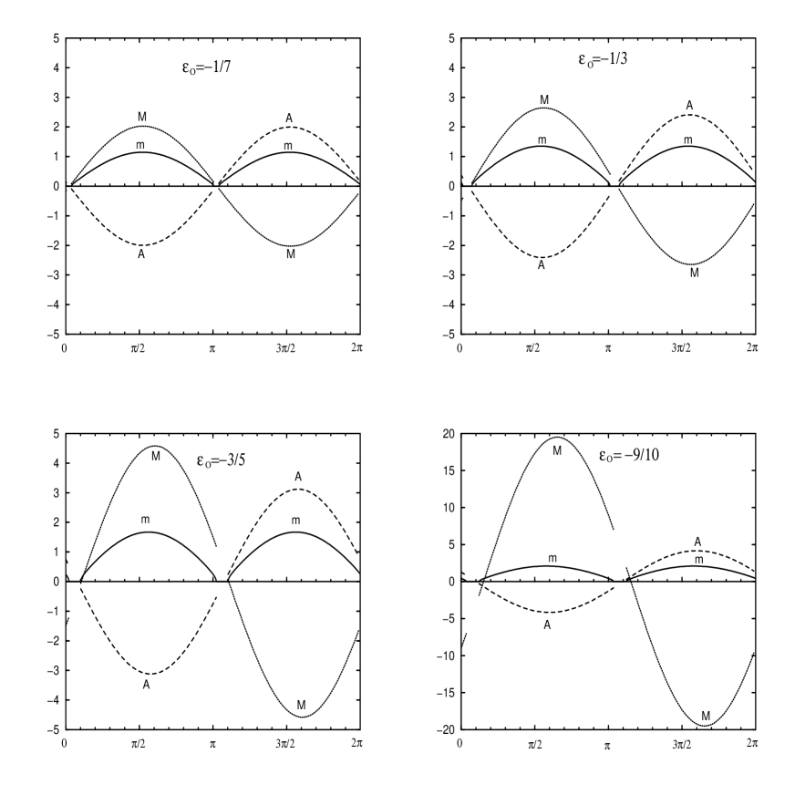
Figure 4: Soft parameters in units of $m_{3/2}$ versus $\theta$ for different values of $\epsilon_{O}$ in the non–standard embedding case. Here $M$, $m$ and $A$ are the gaugino mass, the scalar mass and the trilinear parameter respectively.

This result is to be compared with the one of [13] where the standard-embedding soft terms were analyzed. From Fig. 1 of that paper, where cases $\epsilon_{O}=1/7,1/3,3/5,1$ where shown, we see that the forbidden ranges of $\theta$ are now substantially decreased For example, whereas the dilaton–dominated case, $|\sin\theta|=1$ is always allowed, in the standard–embedding situation it may be forbidden depending on the value of $\epsilon_{O}$. Also we see that the range of soft terms is now substantially increased. In the limit $\epsilon_{O}\rightarrow-1$, $0.3<|A|/m_{3/2}<4.58$, $0<m/m_{3/2}<2.26$ and $|M|\rightarrow\infty$.

In order to discuss the SUSY spectra further, it is worth noticing that although gaugino masses are in general larger than scalar masses, for values of $\epsilon_{O}$ approaching $-1$ there are two narrow ranges of values of $\theta$ where the opposite situation occurs. This can be seen in Fig. 4 for the cases $\epsilon_{O}=-3/5,-9/10$. Let us remark that $M/m_{3/2}$ and $m/m_{3/2}$ are then very small and therefore $m_{3/2}$ must be large in order to fulfil e.g. the low–energy bounds on gluino masses . These ranges of $\theta$ can be seen in more detail in Fig. 5, where the ratio $m/|M|$ versus $\theta$ is plotted for different values of $\epsilon_{O}$. This result is to be compared with the one of Fig. 3 in [13]. There, the standard embedding case is analyzed and $r\equiv m/|M|<1$ for any value of $\theta$. Fig. 5 also allows us to study some properties of the low–energy ($\approx M_{W}$) spectra independently of the details of the electroweak breaking using the formula (see e.g. [13])

$$M_{\tilde{g}}:m_{\tilde{Q}_{L}}:m_{\tilde{u}_{R}}:m_{\tilde{d}_{R}}:m_{\tilde{L}_{L}}:m_{\tilde{e}_{R}}$$

$$\approx 1:\frac{1}{3}\sqrt{7.6+r^{2}}:\frac{1}{3}\sqrt{7.17+r^{2}}:\frac{1}{3}\sqrt{7.14+r^{2}}:\frac{1}{3}\sqrt{0.53+r^{2}}:\frac{1}{3}\sqrt{0.15+r^{2}}\ ,$$ (2.38)

where $\tilde{g}$ denote the gluino, $\tilde{l}$ all the sleptons and $\tilde{q}$ first and second generation squarks. Most values of $\theta$ imply $r<1$ and from (2.38) we obtain

$$M_{\tilde{g}}\approx m_{\tilde{q}}>m_{\tilde{l}}\ .$$ (2.39)

This is also the generic (tree–level) result in Calabi–Yau compactifications of the weakly–coupled heterotic string, which can be recovered from (2.30) by taking the limit $(T+\bar{T})<<(S+\bar{S})$, i.e. $\epsilon_{O}\rightarrow 0$. Then $M=\sqrt{3}m=\sqrt{3}m_{3/2}\sin\theta$ [40] implying $r=1/\sqrt{3}$ except in the limit $\sin\theta\rightarrow 0$ which is not well defined. Only in this limit one might expect $r>1$, similarly to what happens in the orbifold case, due to string loop corrections. This is something to be checked [51].

However, when $\epsilon_{O}$ is approaching $-1$ the above situation (2.39) concerning Fig. 5 can be reversed since

$$M_{\tilde{g}}<m_{\tilde{q}}\approx m_{\tilde{l}}\ ,$$ (2.40)

for $\theta$ in the narrow ranges where $r>1$.

Finally, notice that in the case $\beta_{O}=0$, i.e. $\epsilon_{O}=0$, which corresponds to the straight line $m/|M|=1/\sqrt{3}$, the phenomenologically interesting sum–rule $\sum_{i=1}^{3}m_{i}^{2}=M^{2}$ [52] is trivially fulfilled. Moreover, it is also fulfilled for any other possible value of $\epsilon_{O}$ when $\theta=\pi/6$ (and $\pi/6+\pi$) since then the $\epsilon_{O}$ contribution in (2.30) is cancelled and one obtains $m=m_{3/2}/2$ and $|M|=\sqrt{3}m_{3/2}/2$. See also in Fig. 5 how all graphs intersect each other at those angles. Since this result is independent on the value of $\epsilon_{O}$, it happened also for $0<\epsilon_{O}<1$ (see Fig. 3 in [13]).

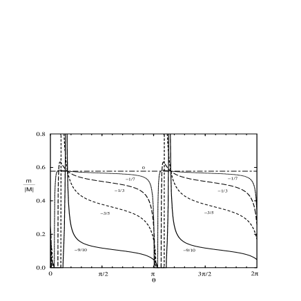
Figure 5: $m/|M|$ versus $\theta$ for different values of $\epsilon_{O}$ in the non–standard embedding case.

3 Vacua with five-branes

In the previous section, we studied the phenomenology of heterotic M–theory vacua obtained through standard and non–standard embeddings. Here we want to analyze (non–perturbative) heterotic M–theory vacua due to the presence of five–branes [3]. As mentioned in the introduction, five–branes are non–perturbative objects, located at points, $x^{11}=x_{n}(n=1,...,N)$, throughout the orbifold interval. The modifications to the four–dimensional effective action determined by (2.5), (2.6) and (2.7), due to their presence, have recently been investigated by Lukas, Ovrut and Waldram [26, 23]. Basically, they are due to existence of moduli, $Z_{n}$, whose ${\rm Re}(Z_{n})\equiv z_{n}=x_{n}/\pi\rho\in(0,1)$ are the five–brane positions in the normalized orbifold coordinates. Then, the effective supergravity obtained from heterotic M–theory compactified on a Calabi–Yau manifold in the presence of five–branes is now determined by

$$K = -\ln(S+\bar{S})-3\ln(T+\bar{T})+K_{5}+\frac{3}{T+\bar{T}}\left(1+\frac{1}{3}e_{O}\right)H_{pq}C_{O}^{p}\bar{C}_{O}^{q},$$

$$f_{O} = S+B_{O}T\ ,\quad f_{H}=S+B_{H}T\ ,$$

$$W_{O} = d_{pqr}C_{O}^{p}C_{O}^{q}C_{O}^{r}\ ,$$ (3.1)

with

$$e_{O}=b_{O}\frac{T+\bar{T}}{S+\bar{S}}\ .$$ (3.2)

Here $K_{5}$ is the Kähler potential for the five–brane moduli $Z_{n}$, $H_{pq}$ is some $T$–independent metric and

$$b_{O} = \beta_{O}+\sum_{n=1}^{N}(1-z_{n})^{2}\beta_{n}\ ,$$

$$B_{O} = \beta_{O}+\sum_{n=1}^{N}(1-Z_{n})^{2}\beta_{n}\ ,$$

$$B_{H} = \beta_{H}+\sum_{n=1}^{N}(Z_{n})^{2}\beta_{n}\ ,$$ (3.3)

with $\beta_{O}$, $\beta_{H}$ the instanton numbers and $\beta_{n}$ the five–brane charges. The former, instead of constraint (2.20), must fulfil the following constraint:

$$\beta_{O}+\sum_{n=1}^{N}\beta_{n}+\beta_{H}=0\ .$$ (3.4)

It is worth noticing that in addition to the observable and hidden sector gauge groups, $G_{O}$ and $G_{H}$, there appear gauge groups from the five–branes. Thus the total gauge group at low energies is in fact $G_{O}\times G_{H}\times G_{1}\times...\times G_{N}$ [26, 23]. We are assuming here that $G_{O}$ arises from one of the $E_{8}$ groups. In this sense the five–brane sectors are considered hidden sector interacting with the observable sector only through bulk supergravity.

Let us also remark that we are considering, as in the previous section, a compactification on a Calabi–Yau manifold with only one Kähler modulus $h_{1,1}=1$. As discussed in the introduction, such Calabi–Yau spaces exist and their phenomenological properties are extremely interesting.

Assuming for simplicity that $<Z_{n}>=<z_{n}>$, i.e. $<B_{O}>=<b_{O}>$, the set of eqs. (2.9)–(2.14) is still valid with the modification $\epsilon_{O,H}\rightarrow e_{O,H}$, where

$$e_{H}=b_{H}\frac{T+\bar{T}}{S+\bar{S}}\ ,$$ (3.5)

with

$$b_{H}=\beta_{H}+\sum_{n=1}^{N}(z_{n})^{2}\beta_{n}\ .$$ (3.6)

Following the analysis of subsection 2.2 we can write $e_{O}$ as

$$e_{O}=\frac{4-(S+\bar{S})}{(S+\bar{S})}\ ,$$ (3.7)

and therefore Fig. 1 is still valid substituying $\epsilon_{O}$ by $e_{O}$. We can obtain different bounds on $e_{O}$ depending on the sign of both $b_{O}$ and $b_{H}$:

i) $b_{H}\geq 0$, $b_{O}\leq 0$

Then $e_{H}$ is positive and $e_{O}$ negative. Since $V_{O}=V(1+e_{O})$ must be positive we need

$$-1<e_{O}\leq 0\ .$$ (3.8)

ii) $b_{H}\geq 0$, $b_{O}>0$

Now since $e_{O}$ is positive $V_{O}$ will always be positive and therefore the only bound is

$$0<e_{O}\ .$$ (3.9)

iii) $b_{H}<0$, $b_{O}>0$

In this case $e_{H}$ is negative. Since $V_{H}=V(1+e_{H})$ must be positive we need $e_{H}>-1$. On the other hand, using (3.2) and (3.5), $e_{O}=e_{H}\frac{b_{O}}{b_{H}}$ and as a consequence the following bounds are obtained

$$0<e_{O}<\frac{b_{O}}{|b_{H}|}\ .$$ (3.10)

iv) $b_{H}<0$, $b_{O}\leq 0$

Now both $e_{O}$ and $e_{H}$ are negative. To avoid negative volumes we need $e_{O}>-1$ and $e_{H}>-1$. As discussed above we can write $e_{O}=e_{H}\frac{b_{O}}{b_{H}}$ and therefore two possibilities arise:

If $|b_{O}|\geq|b_{H}|$

$$-1<e_{O}\leq 0\ .$$ (3.11)

If $|b_{O}|<|b_{H}|$

$$-\frac{b_{O}}{b_{H}}<e_{O}\leq 0\ .$$ (3.12)

For instance, for the example studied in [26] where there are four five–branes at $(z_{1},z_{2},z_{3},z_{4})=(0.2,0.6,0.8,0.8)$ with charges $(\beta_{1},\beta_{2},\beta_{3},\beta_{4})=(1,1,1,1)$ and instanton number $(\beta_{O},\beta_{H})=(-1,-3)$, one obtains $b_{O}=-0.12$, $b_{H}=-1.32$ and then one should apply (3.12) with the result $-0.09\stackrel{{\scriptstyle\scriptstyle<}}{{\scriptstyle\sim}}e_{O}\stackrel{{\scriptstyle\scriptstyle<}}{{\scriptstyle\sim}}0$.

The standard and non–standard embeddings studied in section 2 are particular cases of this more general analysis with five–branes. For $\beta_{n}=0$ in (3.3) and (3.4), i.e. no five–branes, we have $b_{O}=\beta_{O}=-\beta_{H}=-b_{H}$ and $e_{O}=\epsilon_{O}$. If $\beta_{O}<0$, from i) we recover the non–standard embedding case, $-1<\epsilon_{O}<0$. This is the part of the graph corresponding to $S+\bar{S}>4$ shown in Fig. 1. For $\beta_{O}>0$, from iii) we recover the standard embedding (and also some non–standard embedding) case since $0<\epsilon_{O}<1$ This is the part of the graph corresponding to $2<S+\bar{S}<4$ shown in Fig. 1. It is worth noticing that the values $0<(S+\bar{S})<2$, corresponding to $\epsilon_{O}>1$, which are not possible in the absence of five–branes, are allowed in their presence since $e_{O}>1$ is possible (cases ii) and iii)).

3.1 Scales

In the presence of five–branes (2.25) is no longer true since (2.11) and (2.14) are modified in the following way: $V_{O}=V(1+e_{O})$ and $V_{H}=V(1+e_{H})$. Therefore

$$<V>=V\left(1+\frac{e_{O}+e_{H}}{2}\right)\ .$$ (3.13)

Then the relevant formulae to study the relation between the different scales of the theory are (2.17) and (2.19) with the modification $\epsilon_{O}\rightarrow e_{O}$. Notice that (2.18) is not modified. Similarly to the case without five–branes, to obtain $V_{O}^{-1/6}\approx 3\times 10^{16}$ GeV when $T+\bar{T}$ and $S+\bar{S}$ are of order one is quite natural. This can be seen from (2.17)

$$V_{O}^{-1/6} = \left(\frac{1}{1+\frac{e_{O}}{2}\left(1+\frac{b_{H}}{b_{O}}\right)}\right)^{1/2}3.6\times 10^{16}\left(\frac{4}{S+\bar{S}}\right)^{1/2}\left(\frac{2}{T+\bar{T}}\right)^{1/2}\left(\frac{1}{1+e_{O}}\right)^{1/6}{\rm GeV}$$

(3.14)

where (3.13) with (3.5) and (3.2) has been used. Using (3.2) and (3.7) it is interesting to write (3.14) as

$$V_{O}^{-1/6} = \left(\frac{1}{1+\frac{e_{O}}{2}\left(1+\frac{b_{H}}{b_{O}}\right)}\right)^{1/2}3.6\times 10^{16}\left(\frac{b_{O}}{2e_{O}}\right)^{1/2}\left(1+e_{O}\right)^{5/6}{\rm GeV}\ .$$ (3.15)

In the left hand side of the Fig. 6a we show an example of the case i), $b_{O}=-7/4$ and $b_{H}=5/4$, corresponding to $-1<e_{O}<0$. In the right hand side we show an example of the case ii), $b_{O}=b_{H}=1/2$, corresponding to $e_{0}>0$. Both are interesting examples since they cover the whole range of validity of $e_{O}$ and will be used below to study the soft terms. Unlike the standard and non–standard embedding cases with $\beta_{O}>0$ shown in the right hand side of Fig. 2, now the line corresponding to $V_{O}^{-1/6}$ intersects easily the straight line corresponding to the GUT scale. This is obtained for $e_{O}=0.46$ which, using (3.7) and (3.2), corresponds to $S+\bar{S}=2.73$ and $T+\bar{T}=2.54$. Of course this effect is due essentially to the extra factor appearing in (3.15), coming from the average volume, with respect to (2.29).

Figure 6: $\log M_{11}$, $\log V_{O}^{-1/6}$ and $\log(\pi\rho)^{-1}$ versus (a) $e_{O}$ and (b) $\log e_{O}$ in the cases $b_{O}=b_{H}=1/2$ (for $0<e_{O}$) and $b_{O}=-7/4$, $b_{H}=5/4$ (for $-1<e_{O}<0$). The straight line indicates the phenomenologically favored GUT scale, $M_{GUT}=3\times 10^{16}$ GeV.

Only in some special limits one may lower the scales. As in the case without fivebranes, fine–tuning $e_{O}\rightarrow-1$ we are able to obtain $V_{O}^{-1/6}$ as low as we wish. The numerical results will be basically similar to the ones of non–standard embedding in subsection 2.3.1

Moreover, $e_{O}>1$ is possible in the presence of five–branes. Therefore with $e_{O}$ sufficiently large we may get $V_{O}^{-1/6}$ very small. This is shown in Fig. 6b. For example, with $\log e_{O}=56.1$ the experimental lower bound $(\pi\rho)^{-1}=10^{-13}$ GeV is obtained for $V_{O}^{-1/6}=8\times 10^{6}$ GeV, corresponding to $S+\bar{S}=3.1\times 10^{-56}$ and $T+\bar{T}=8$. Clearly we introduce a hierarchy problem.

Figure 7: $\log M_{11}$, $\log V_{O}^{-1/6}$ and $\log(\pi\rho)^{-1}$ versus $\log(T+\bar{T})$ for the case $b_{O}=0$. The straight line indicates the phenomenologically favored GUT scale, $M_{GUT}=3\times 10^{16}$ GeV.

Finally, Let us analyze the special case $b_{O}=0$. The analysis will be similar to the one of the case $\beta_{O}=0$ without five–branes in subsection 2.3.1. Since $e_{O}$ in (3.2) is vanishing and using (3.7), $S+\bar{S}=4$, eq. (2.17) can be written as

$$V_{O}^{-1/6} = \left(\frac{1}{1+\frac{1}{8}b_{H}(T+\bar{T})}\right)^{1/2}3.6\times 10^{16}\left(\frac{2}{T+\bar{T}}\right)^{1/2}{\rm GeV}\ ,$$ (3.16)

where (3.5) has been used. Depending on the value of $b_{H}$ we obtain different results. If $b_{H}=0$, eq. (2.37) is recovered and therefore we obtain the same results as in the case $\beta_{O}=\beta_{H}=0$ without five–branes (see Fig. 3). If $b_{H}>0$ the results are qualitatively similar, the larger $T+\bar{T}$ the smaller $V_{O}^{-1/6}$ becomes. However, notice that now for large $T$ we have a factor $(T+\bar{T})^{-1}$ and then not so large values of $T+\bar{T}$ as in Fig. 3 are needed in order to lower the scales. This is shown in Fig. 7 for the case $b_{H}=1$. Then $V_{O}^{-1/6}=1$ TeV can be obtained for $T+\bar{T}=10^{14}$ with the size of the orbifold $(\pi\rho)^{-1}=5\times 10^{-12}$ GeV close to its experimental bound of $1$ millimetre. In any case, still a large hierarchy between $S+\bar{S}$ and $T+\bar{T}$ is needed. Finally, for $b_{H}<0$ we are in the case iv) and therefore we have the constraint $0<(T+\bar{T})<4/|b_{H}|$, implying that $V_{O}^{-1/6}$ around the GUT scale can be obtained but lowering it to intermediate or $1$ TeV values is not possible.

3.2 Soft terms

Let us now concentrate on the computation of soft terms. The above supergravity model (3.1) gives rise to the following gaugino masses, scalar masses and trilinear parameters:

$$M = \frac{1}{(S+\bar{S})(1+\frac{B_{O}T+\bar{B}_{O}\bar{T}}{S+\bar{S}})}\left(F^{S}+F^{T}B_{O}+TF^{n}{\partial_{n}}{B_{O}}\right)\ ,$$

$$m^{2} = V_{0}+m_{3/2}^{2}-\frac{1}{(3+e_{O})^{2}}\left[e_{O}(6+e_{O})\frac{|F^{S}|^{2}}{(S+\bar{S})^{2}}\right.$$

$$+3(3+2e_{O})\frac{|F^{T}|^{2}}{(T+\bar{T})^{2}}-\frac{6e_{O}}{(S+\bar{S})(T+\bar{T})}{\rm Re\,}F^{S}\bar{F}^{\bar{T}}$$

$$+\left(\frac{e_{O}}{b_{O}}(3+e_{O})\partial_{n}\partial_{\bar{m}}b_{O}-\frac{e_{O}^{2}}{b_{O}^{2}}\partial_{n}b_{O}\partial_{\bar{m}}b_{O}\right)F^{n}\bar{F}^{\bar{m}}$$

$$\left.-\frac{6e_{O}}{b_{O}}\frac{\partial_{\bar{n}}b_{O}}{S+\bar{S}}{\rm Re\,}F^{S}\bar{F}^{\bar{n}}+\frac{6e_{O}}{b_{O}}\frac{\partial_{\bar{n}}b_{O}}{T+\bar{T}}{\rm Re\,}F^{T}\bar{F}^{\bar{n}}\right]\ ,$$

$$A = -\frac{1}{3+\epsilon_{O}}\left[(3-2e_{O})\frac{F^{S}}{S+\bar{S}}+3e_{O}\frac{F^{T}}{T+\bar{T}}\right.$$ (3.17)

$$+\left.\left(\frac{3e_{O}}{b_{O}}\partial_{n}b_{O}-(3+e_{O}){\partial_{n}}K_{5}\right)F^{n}\right]\ ,$$

where $\partial_{n}\equiv\frac{\partial}{\partial Z_{n}}$ and for the moment we write explicitly the $F$–terms of the dilaton ($F^{S}$), modulus ($F^{T}$) and five–branes ($F^{n}$). They must fulfil the relation

$$V_{0}=\frac{|F^{S}|^{2}}{(S+\bar{S})^{2}}+\frac{3|F^{T}|^{2}}{(T+\bar{T})^{2}}+\bar{F}^{\bar{n}}F^{m}\partial_{\bar{n}}\partial_{m}K_{5}-3m_{3/2}^{2}\ .$$ (3.18)

Assuming, as in subsection 2.2.2, that the source of the $\mu$ term is a bilinear piece in the superpotential and/or the Kähler potential, the result is

$$B = \hat{\mu}^{-1}\left(\frac{T+\bar{T}}{3+e_{O}}\right)\left\{\frac{\bar{W}(\bar{S},\bar{T})}{|W(S,T)|}\ (S+\bar{S})^{-1/2}(T+\bar{T})^{-3/2}e^{K_{5}/2}\mu\right.$$

$$\left[F^{S}\left(\frac{-1}{S+\bar{S}}+\right.\right.\left.\partial_{S}\log\mu+\frac{2e_{O}}{3+e_{O}}\frac{1}{S+\bar{S}}\right)+F^{T}\left(\frac{-3}{T+\bar{T}}+\right.\partial_{T}\log\mu$$

$$\left.+\frac{6}{3+e_{O}}\frac{1}{T+\bar{T}}\right)+F^{n}\left(\partial_{n}K_{5}+\partial_{n}\log\mu-\frac{2\partial_{n}b_{O}}{3+e_{O}}\right.\left.\frac{T+\bar{T}}{S+\bar{S}}\right)-\left.m_{3/2}\right]$$

$$+(2m_{3/2}^{2}+V_{0})Z-m_{3/2}\left(\bar{F}^{\bar{S}}\partial_{\bar{S}}Z+\right.\left.\bar{F}^{\bar{T}}\partial_{\bar{T}}Z+\bar{F}^{\bar{n}}\partial_{\bar{n}}Z\right)$$

$$+m_{3/2}\left[F^{S}\left(\partial_{S}Z+\frac{2e_{O}}{3+e_{O}}\right.\right.\left.\frac{1}{S+\bar{S}}Z\right)+F^{T}\left(\partial_{T}Z+\frac{6}{3+e_{O}}\right.\left.\frac{1}{T+\bar{T}}Z\right)$$

$$+F^{n}\left(\partial_{n}Z-\frac{2\partial_{n}b_{O}}{3+e_{O}}\right.\left.\left.\frac{T+\bar{T}}{S+\bar{S}}Z\right)\right]-|F^{S}|^{2}\left(\partial_{S}\partial_{\bar{S}}Z+\frac{2e_{O}}{3+e_{O}}\frac{\partial_{\bar{S}}Z}{S+\bar{S}}\right)$$

$$-|F^{T}|^{2}\left(\partial_{T}\partial_{\bar{T}}Z+\frac{6}{3+e_{O}}\frac{\partial_{\bar{T}}Z}{T+\bar{T}}\right)-\bar{F}^{\bar{n}}F^{m}\left(\partial_{m}\partial_{\bar{n}}Z-\frac{2\partial_{m}b_{O}}{3+e_{O}}\right.\left.\frac{T+\bar{T}}{S+\bar{S}}\partial_{\bar{n}}Z\right)$$

$$-\bar{F}^{\bar{S}}F^{T}\left(\partial_{T}\partial_{\bar{S}}Z+\frac{6}{3+e_{O}}\frac{\partial_{\bar{S}}Z}{T+\bar{T}}\right)-\bar{F}^{\bar{T}}F^{S}\left(\partial_{S}\partial_{\bar{T}}Z+\frac{2e_{O}}{3+e_{O}}\frac{\partial_{\bar{T}}Z}{S+\bar{S}}\right)$$

$$-\bar{F}^{\bar{S}}F^{n}\left(\partial_{n}\partial_{\bar{S}}Z-\frac{2\partial_{n}b_{O}}{3+e_{O}}\right.\left.\frac{T+\bar{T}}{S+\bar{S}}\partial_{\bar{S}}Z\right)-\bar{F}^{\bar{n}}F^{S}\left(\partial_{S}\partial_{\bar{n}}Z+\frac{2e_{O}}{3+e_{O}}\frac{\partial_{\bar{n}}Z}{S+\bar{S}}\right)$$

$$-\bar{F}^{\bar{T}}F^{n}\left(\partial_{n}\partial_{\bar{T}}Z-\frac{2\partial_{n}b_{O}}{3+e_{O}}\right.\left.\frac{T+\bar{T}}{S+\bar{S}}\partial_{\bar{T}}Z\right)-\bar{F}^{\bar{n}}F^{T}\left.\left(\partial_{T}\partial_{\bar{n}}Z+\frac{6}{3+e_{O}}\frac{\partial_{\bar{n}}Z}{T+\bar{T}}\right)\right\}\ ,$$

with the effective $\mu$ parameter given by:

$$\hat{\mu} = \left(\frac{T+\bar{T}}{3+e_{O}}\right)\left(\frac{\bar{W}(\bar{S},\bar{T})}{|W(S,T)|}(S+\bar{S})^{-1/2}(T+\bar{T})^{-3/2}e^{K_{5}/2}\mu\right.+m_{3/2}Z$$ (3.20)

$$\left.-\bar{F}^{\bar{S}}\partial_{\bar{S}}Z-\bar{F}^{\bar{T}}\partial_{\bar{T}}Z-\bar{F}^{\bar{n}}\partial_{\bar{n}}Z\right)$$

Due to the possible contribution of several $F$–terms associated with five–branes, which can have in principle off–diagonal Kähler metrics, the numerical computation of the soft terms turns out to be extremely involved. In order to get an idea of their value and also to study the deviations with respect to the case without five–branes we can do some simplifications. One possibility is to assume that five–branes are present but only the $F$–terms associated with the dilaton and the modulus contribute to supersymmetry breaking, i.e. $F^{n}=0$. Then, assuming as before $<Z_{n}>=<z_{n}>$ and using parametrization (2.33), eq. (3.17) reduces to eq. (2.30) with $e_{O}$ instead of $\epsilon_{O}$. Under these simplifying assumptions, Figs. 4 and 5 in section 2 (and Figs. 1 and 3 in [13]) are also valid in this case since, as discussed above the range of allowed values of $e_{O}$ includes those of $\epsilon_{O}$, i.e. $-1<e_{O}<1$. The relevant difference with respect to the case without five–branes is that now values with $e_{O}\geq 1$ are allowed. We plot this possibility in Figs. 8 and 9 for some values of $e_{O}$. Fig. 8 shows that the range of $\theta$ forbidden by having a negative scalar mass–squared, is large and quite stable against variations of $e_{O}$. This pattern of soft terms is qualitatively different from that without five–branes analyzed in subsection 2.3 for the non–standard embedding and in Fig. 1 of [13] for the standard embedding. However, the fact that always scalar masses are smaller than gaugino masses in the latter case (see Fig. 3 in [13]) is also true here. In Fig. 9 we show the ratio $m/|M|$ versus $\theta$ for different values of $e_{O}$. Although the larger the value of $e_{O}$, the larger the ratio becomes, there is an upper bound $m/|M|=1$ (obtained for $\theta=0$). As discussed in (2.39) we will obtain at low–energies, $M_{\tilde{g}}\approx m_{\tilde{q}}>m_{\tilde{l}}$. Notice that the sum–rule $3m^{2}=M^{2}$ is also fulfilled for $\theta=\pi/6$ (and $\pi/6+\pi$).

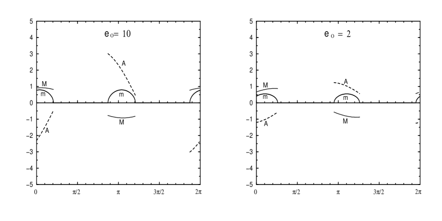
Figure 8: Soft parameters in units of $m_{3/2}$ versus $\theta$ for different values of $e_{O}$ when five–branes are present without contributing to supersymmetry breaking.

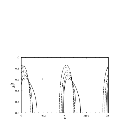
Figure 9: $m/|M|$ versus $\theta$ for different values of $e_{O}$ when five–branes are present without contributing to supersymmetry breaking.

Another possibility to simplify the numerical computation of the soft terms is to assume that there is only one five–brane in the model. For example, parametrizing consistently with (3.18)

$$F^{S} = \sqrt{3}m_{3/2}C(S+\bar{S})\sin\theta\cos\theta_{1}e^{-i\gamma_{S}}\ ,$$

$$F^{T} = m_{3/2}C(T+\bar{T})\cos\theta\cos\theta_{1}e^{-i\gamma_{T}}\ ,$$

$$F^{1} = \sqrt{3}m_{3/2}C({{\partial}_{1}{\partial}_{\bar{1}}K_{5}})^{-1/2}sin\theta_{1}e^{-i\gamma_{1}}\ ,$$ (3.21)

where $\theta_{1}$ is the new goldstino angle associated to the $F$–term of the five–brane $F^{1}$, we obtain from (3.17)

$$M = \frac{\sqrt{3}m_{3/2}C}{\left(1+\frac{B_{O}T+\bar{B}_{O}\bar{T}}{S+\bar{S}}\right)}\left(\sin\theta\cos\theta_{1}e^{-i\gamma_{S}}+\frac{1}{\sqrt{3}}B_{O}\frac{e_{O}}{b_{O}}\cos\theta\cos\theta_{1}e^{-i\gamma_{T}}\right.$$

$$\left.-\frac{2T}{S+\bar{S}}(1-Z_{1})\beta_{1}({{\partial}_{1}{\partial}_{\bar{1}}K_{5}})^{-1/2}sin\theta_{1}e^{-i\gamma_{1}}\right)\ ,$$

$$m^{2} = V_{o}+m_{3/2}^{2}-\frac{3m_{3/2}^{2}C^{2}}{(3+e_{O})^{2}}\left\{e_{O}(6+e_{O})\sin^{2}\theta\cos^{2}\theta_{1}\right.$$

$$+(3+2e_{O})\cos^{2}\theta\cos^{2}\theta_{1}-2\sqrt{3}e_{O}\sin\theta\cos\theta\cos^{2}\theta_{1}\cos(\gamma_{S}-\gamma_{T})$$

$$+({{\partial}_{1}{\partial}_{\bar{1}}K_{5}})^{-1}\sin^{2}\theta_{1}\left((3+e_{O})\beta_{1}\frac{e_{O}}{2b_{O}}-\left[(1-z_{1})\beta_{1}\frac{e_{O}}{b_{O}}\right]^{2}\right)$$

$$+6(1-z_{1})\beta_{1}\frac{e_{O}}{b_{O}}({{\partial}_{1}{\partial}_{\bar{1}}K_{5}})^{-1/2}\sin\theta\sin\theta_{1}\cos\theta_{1}\cos(\gamma_{1}-\gamma_{S})$$

$$\left.-2\sqrt{3}(1-z_{1})\beta_{1}\frac{e_{O}}{b_{O}}({{\partial}_{1}{\partial}_{\bar{1}}K_{5}})^{-1/2}\cos\theta\sin\theta_{1}\cos\theta_{1}\cos(\gamma_{T}-\gamma_{n})\right\}\ ,$$

$$A = -\frac{\sqrt{3}m_{3/2}C}{3+e_{O}}\left[(3-2e_{O})\sin\theta\cos\theta_{1}e^{-i\gamma_{S}}+\sqrt{3}e_{O}\cos\theta\cos\theta_{1}e^{-i\gamma_{T}}\right.$$ (3.22)

$$\left.-({{\partial}_{1}{\partial}_{\bar{1}}K_{5}})^{-1/2}sin\theta_{1}e^{-i\gamma_{1}}\left((3+e_{O}){{\partial}_{1}K_{5}}+3(1-z_{1})\beta_{1}\frac{e_{O}}{b_{O}}\right)\right]\ .$$

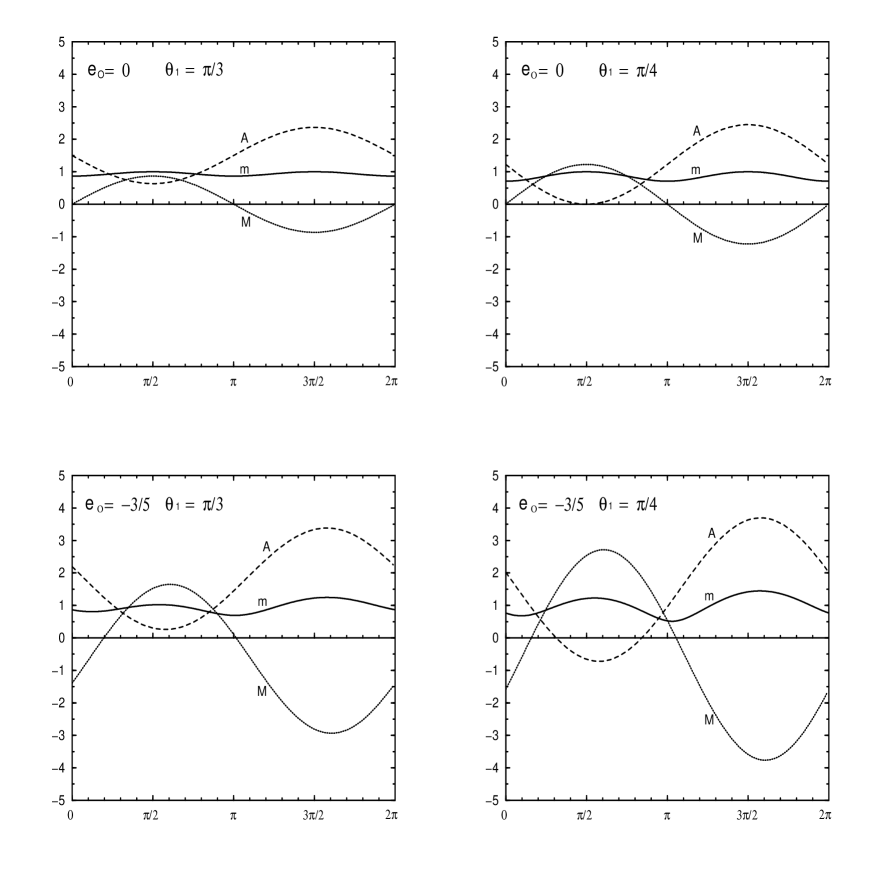
Figure 10: Soft parameters in units of $m_{3/2}$ versus $\theta$ for different values of $e_{O}$ and goldstino angle $\theta_{1}$ when one five–brane is contributing to supersymmetry breaking.

Similarly one can obtain the $B$ parameter using (3.2).

Unfortunately, the numerical analysis of this simplified case is not straightforward. All soft terms depend not only on the new goldstino angle $\theta_{1}$ in addition to $m_{3/2}$, $\theta$ and $e_{O}$, but also on other free parameters. For example, although gaugino masses can be further simplified with the assumption $<Z_{n}>=<z_{n}>$, i.e. $<B_{O}>=<\bar{B}_{O}>=<b_{O}>$, and $<T>=<\bar{T}>$

$$M = \frac{\sqrt{3}m_{3/2}C}{1+e_{O}}\{\sin\theta\cos\theta_{1}e^{-i\gamma_{S}}+\frac{1}{\sqrt{3}}e_{O}\cos\theta\cos\theta_{1}e^{-i\gamma_{T}}$$ (3.23)

$$-\frac{e_{O}}{b_{O}}(1-z_{1})\beta_{1}({{\partial}_{1}{\partial}_{\bar{1}}K_{5}})^{-1/2}sin\theta_{1}e^{-i\gamma_{1}}\}\ ,$$

still they have an explicit dependence on $z_{1}$ and $\partial_{1}\partial_{\bar{1}}K_{5}$. Notice that, for a given model, $\beta_{O}$ and $\beta_{1}$ are known and therefore $b_{O}$ can be computed from (3.3) once $z_{1}$ is fixed. Something similar occurs for the $A$ parameter, where $z_{1}$, $\partial_{1}K_{5}$ and $\partial_{1}\partial_{\bar{1}}K_{5}$ appear explicitly, and for the scalar masses, where $z_{1}$ and $\partial_{1}\partial_{\bar{1}}K_{5}$ also appear. Thus in order to compute soft terms when a five–brane is present and contributing to supersymmetry breaking we have to input these values. Fortunately, $z_{1}$ is in the range $(0,1)$ and, although $K_{5}$ is not known, since it depends on $z_{1}$, we expect $\partial_{1}K_{5}$, $\partial_{1}\partial_{\bar{1}}K_{5}={\cal O}(1)$. So we can consider the following representative example: $z_{1}=1/2$ and $\partial_{1}K_{5}=\partial_{1}\partial_{\bar{1}}K_{5}=1$. Since, still we have to input the value of $b_{O}$, we choose the interesting example with $\beta_{O}=-2$ and $\beta_{1}=1$ which implies $b_{O}=-7/4$. In this way, using (3.4) and (3.6), $b_{H}$ is also fixed, $b_{H}=5/4$, and from the result (3.8) in case i) we know that the whole range of allowed (negative) values of $e_{O}$ can be analyzed.

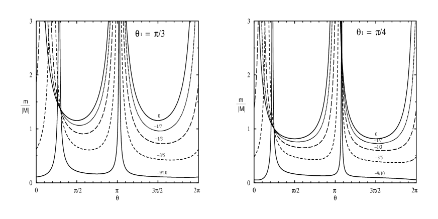
Figure 11: $m/|M|$ versus $\theta$ for different values of $e_{O}$ and goldstino angle $\theta_{1}$ when one five–brane is contributing to supersymmetry breaking.

Figure 12: (a) Soft parameters in units of $m_{3/2}$ and (b) $m/|M|$ versus $e_{O}$, when only the five–brane contributes to supersymmetry breaking with $\theta_{1}=\pi/2$.

Taking into account again the current experimental limits, we will assume $V_{0}=0$ and $\gamma_{S}=\gamma_{T}=\gamma_{1}=0\ ({\rm mod}\ \,\pi)$. More specifically we will set $\gamma_{S}$, $\gamma_{T}$ and $\gamma_{1}$ to zero and allow $\theta$ and $\theta_{1}$ to vary in a range $[0,2\pi)$. We show in Fig. 10 the dependence on $\theta$ of the soft terms in units of the gravitino mass for some values of $e_{O}$ and $\theta_{1}$. Due to the contribution of $\theta_{1}$ to the soft terms (3.22) the shift $\theta\rightarrow\theta+\pi$ does not imply, as in Figs. 4 and 8, $m\rightarrow m$, $M\rightarrow-M$ and $A\rightarrow-A$. However, this is still true for $\theta_{1}\rightarrow\theta_{1}+\pi$. Besides, under the shifts $\theta_{1}\rightarrow\pi-\theta_{1}$ and $\theta\rightarrow\theta+\pi$, $m$, $M$ and $A$ remain invariant. Therefore from the analysis of the figures corresponding to $\theta_{1}\in[0,\pi/2]$ the rest of the figures can easily be deduced. In particular, in Fig. 10 we plot the values of $\theta_{1}$, $\pi/4$ and $\pi/3$. For a fixed value of $\theta_{1}$, as in the case without five–branes shown in Fig. 4 (with $\epsilon_{O}$ instead of $e_{O}$), the smaller the value of $e_{O}$ the larger the range of soft terms becomes. However, unlike Fig. 4, in Fig. 10 we see a remarkable fact: scalar masses larger than gaugino masses can easily be obtained. This happens not only for narrow ranges of $\theta$ but even for the whole range (see the figure with $e_{O}=0$ and $\theta_{1}=\pi/3$). We can see this in more detail in Fig. 11 where $m/|M|$ versus $\theta$ is plotted.

For example, $m/|M|>1$ can be obtained, for any value of $\theta$, for values of $e_{O}$ close to zero in the case $\theta_{1}=\pi/3$. Moreover, larger values of $\theta_{1}$ allow larger ranges of $e_{O}$ with $m/|M|>1$ for any value of $\theta$. For example, in the limiting case where supersymmetry is only broken by the $F$–term of the five–brane $F^{1}$, i.e. $\theta_{1}=\pi/2$, $m/|M|>1$ for $e_{O}>-0.65$. This case is shown in Fig. 12, where the soft terms and $m/|M|$ versus $e_{O}$ are plotted. Of course, the figures are independent on $\theta$. Let us remark that scalar masses larger than gaugino masses are not easy to obtain, as discussed below (2.39), in the weakly–coupled heterotic string.

It is worth noticing that the sum rule studied above, $3m^{2}=M^{2}$ for $\theta=\pi/6$ (and $\pi/6+\pi$) is no longer true when five–branes contributing to supersymmetry breaking are present.

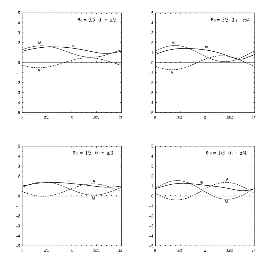
Figure 13: The same as Fig. 10 but for positive values of $e_{O}$.

Finally, let us mention that a different value for $\partial_{1}K_{5}$ that the one considered here, will only modify the expression of the $A$ parameter, since it is the only one which depends on that derivative. On the other hand, one can check that a different value for $\partial_{1}\partial_{\bar{1}}K_{5}$ will not modify the qualitative results concerning gaugino and scalar masses. Notice also that $\partial_{1}\partial_{\bar{1}}K_{5}$ appears always in the denominator in the expressions of the soft terms. So, the larger the value of $\partial_{1}\partial_{\bar{1}}K_{5}$ the smaller the deviation with respect to the case without five–branes becomes. One can also check that different values for $z_{1}$, $\beta_{O}$ and $\beta_{H}$ will not modify the qualitative results concerning gaugino and scalar masses.

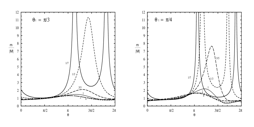
Figure 14: The same as Fig. 11 but for positive values of $e_{O}$.

Figure 15: The same as Fig. 12 but for positive values of $e_{O}$.

We have not analyzed yet positive values of $e_{O}$ in the presence of a five–brane contributing to supersymmetry breaking. In order to carry it out we choose now $\beta_{O}=1$ and $\beta_{1}=-2$ which implies $b_{O}=b_{H}=1/2$. From (3.9) in case ii) we deduce that the whole range of allowed (positive) values of $e_{O}$ can be studied. We show in Fig. 13 the soft terms for the values $e_{O}=1/3,3/5$. For a fixed value of $\theta_{1}$, the larger the value of $e_{O}$ the larger the range of soft terms becomes, unlike the case without five–branes (see Fig. 1 in [13]). On the other hand, scalar masses larger than gaugino masses can also be easily obtained as in the case with negative values of $e_{O}$ studied above. This is plotted in more detail in Fig. 14 for different values of $e_{O}$. For example, for $e_{O}=1/3$ and $\theta_{1}=\pi/3$, $\theta\approx 3\pi/2$ one obtains $m/|M|\approx 10$. Using (2.38) this result implies a relation of the type (2.40), $m_{\tilde{l}}\approx m_{\tilde{q}}\approx 3.5M_{\tilde{g}}$. In Fig. 15 we show the limiting case where supersymmetry is only broken by the $F$–term of the five–brane.

4 Conclusions

In the present paper we have tried to perform a systematic analysis of the soft supersymmetry breaking terms arising in a Calabi–Yau compactification of the heterotic M–theory, as well as a detailed study of the different scales of the theory. Since, as discussed in the introduction, Calabi–Yau manifolds with only one Kähler modulus $T$ are very interesting from the phenomenological point of view, not only because of their simplicity but also because they might give rise to three–family models with an improvement with respect to the non–universality problem, we have concentrated on these spaces.

The soft terms in the standard and non–standard embedding cases depend explicitly on the gravitino mass $m_{3/2}$, the goldstino angle $\theta$ and the parameter $\epsilon_{O}$ (see (2.8)). The only difference between both cases is the range of values where $\epsilon_{O}$ is valid. $-1<\epsilon_{O}<1$ in the latter and $0<\epsilon_{O}<1$ in the former. This will give rise to different patterns of soft terms. In particular, scalar masses larger than gaugino masses in the non–standard embedding case are allowed (see Fig. 5), for narrow ranges of $\theta$, unlike the standard embedding situation. This has obvious implications for low–energy ($\approx M_{W}$) phenomenology, as discussed in (2.39) and (2.40).

The presence of non–perturbative objects as five–branes in the vacuum modifies the previous analysis substantially. Even if the five–branes do not contribute to supersymmetry breaking the soft terms are modified. Basically, the soft terms are given by the same formulae than in the standard and non–standard embedding but with a new parameter $e_{O}$ (instead of $\epsilon_{O}$), see (3.2), which is valid not only for $-1<e_{O}<1$ but also for $e_{O}\geq 1$. However, although the pattern of soft terms is different, scalar masses larger than gaugino masses are not possible (see Fig. 9) as in the standard embedding situation. Other parameters appear when we allow the five–branes to contribute to supersymmetry breaking. In particular, at least, a new goldstino angle $\theta_{1}$ must be included in the computation of soft terms. In this way, scalar masses larger than gaugino masses can be obtained in a natural way (see Figs. 11 and 14). Depending on the values of $e_{O}$ and $\theta_{1}$, scalars could be heavier than gauginos even in the whole range of $\theta$. As discussed below (2.39) this might be possible in the weakly–coupled heterotic string only for $\sin\theta\rightarrow 0$.

Concerning the scales of the theory, we have discussed in detail the relations between the eleven–dimensional Planck mass, the Calabi–Yau compactification scale and the orbifold scale, taking into account higher order corrections to the formulae. Identifying the compactification scale with the GUT scale, it is easier to obtain the phenomenologically favored value, $M_{GUT}\approx 3\times 10^{16}$ GeV, in the non–standard embedding than in the standard one (see Fig. 2). On the other hand, to lower this scale (and therefore the eleven–dimensional Planck scale which is around two times bigger) to intermediate values $\approx 10^{11}$ GeV or $1$ TeV values or to obtain the radius of the orbifold as large as a millimetre is in principle possible in some special limits. In particular, in the non–standard embedding when $\epsilon_{O}\rightarrow-1$ and also in the case $\beta_{O}=0$ (see Fig. 3). However, the necessity of a fine–tuning in the former and the existence of a hierarchy problem in the latter render these possibilities unnatural. In the presence of five–branes, $M_{GUT}$ can be obtained more easily (see Fig. 6a). Although new possibilities arise in order to lower this scale, in particular when $e_{O}$ is very large (see Fig. 6b), again at the cost of introducing a hughe hierarchy problem.

Note added

As this manuscript was prepared, refs. [54] and [55] appeared. The former discusses some of the issues presented in this work, particularly the scenario of subsection 2.3. The latter also discusses soft terms in the presence of five–branes, however, its numerical analysis concentrates on the dilaton limit with $0<e_{O}<2/3$.

Acknowledgments

The work of D.G. Cerdeño has been supported by a Universidad Autónoma de Madrid grant. The work of C. Muñoz has been supported in part by the CICYT, under contract AEN97-1678-E, and the European Union, under contract ERBFMRX CT96 0090.

References

- [1] For a review, see e.g.: J.H. Schwarz, hep-th/9807135, and references therein.
- [2] P. Hořava and E. Witten, Nucl. Phys. B460 (1996) 506; Nucl. Phys. B475 (1996) 94.
- [3] E. Witten, Nucl. Phys. B471 (1996) 135.
- [4] T. Banks and M. Dine, Nucl. Phys. B479 (1996) 173.
- [5] K. Choi, Phys. Rev. D56 (1997) 6588.
- [6] P. Hořava, Phys. Rev. D54 (1996) 7561.
- [7] H. P. Nilles, M. Olechowski and M. Yamaguchi, Phys. Lett. B415 (1997) 24; Nucl. Phys. B530 (1998) 43.
- [8] Z. Lalak and S. Thomas, Nucl. Phys. B515 (1998) 55.
- [9] A. Lukas, B.A. Ovrut and D. Waldram, Phys. Rev. D57 (1998) 7529.
- [10] I. Antoniadis and M. Quiros, Phys. Lett. B416 (1998) 327; Nucl. Phys. B505 (1997) 109.
- [11] K. Choi, H.B. Kim and H. Kim, Mod. Phys. Lett. A14 (1999) 125.
- [12] B. de Carlos, J.A. Casas and C. Muñoz, Phys. Lett. B299 (1993) 234.
- [13] K. Choi, H.B. Kim and C. Muñoz, Phys. Rev. D57 (1998) 7521.
- [14] T. Li, J.L. Lopez and D.V. Nanopoulos, Mod. Phys. Lett. A12 (1997) 2647.
- [15] D. Bailin, G.V. Kraniotis and A. Love, Phys. Lett. B432 (1998) 90; hep-ph/9812283.
- [16] Y. Kawamura, H.P. Nilles, M. Olechowski and M. Yamaguchi, JHEP 9806 (1998) 008.
- [17] S.A. Abel and C.A. Savoy, Phys. Lett. B444 (1998) 119.
- [18] J.A. Casas, A. Ibarra and C. Muñoz, FTUAM 98/18, hep-ph/9810266, to appear in Nucl. Phys. B.
- [19] C.-S. Huang, T. Li, W. Liao and Q.-S. Yan, MADPH-98-1089, hep-ph/9810412.
- [20] P. Candelas, G. Horowitz, A. Strominger and E. Witten, Nucl. Phys. B258 (1985) 46; B.R. Greene, K. Kirklin, P. Miron and G.G. Ross, Nucl. Phys. B278 (1986) 667.
- [21] J. Distler and B. Greene, Nucl. Phys. B304 (1988) 1; W. Pokorski and G.G. Ross, hep-ph/9809537.
- [22] S. Kachru, Phys. Lett. B349 (1995) 76.
- [23] A. Lukas, B.A. Ovrut and D. Waldram, UPR-828T, hep-th/9901017.
- [24] K. Benakli, Phys. Lett. B447 (1999) 51.
- [25] Z. Lalak, S. Pokorski and S. Thomas, CERN-TH/98-230, hep-ph/9807503.
- [26] A. Lukas, B.A. Ovrut and D. Waldram, UPR-815T, hep-th/9808101.
- [27] K. Benakli, CERN-TH/98-317, hep-ph/9809582.
- [28] S. Stieberger, Nucl. Phys. B541 (1999) 109.
- [29] I. Antoniadis, Phys. Lett. B246 (1990) 377; I. Antoniadis, C. Muñoz and M. Quiros, Nucl. Phys. B397 (1993) 515; I. Antoniadis and K. Benakli, Phys. Lett. B326 (1994) 69.
- [30] E. Caceres, V.S. Kaplunovsky and I.M. Mandelberg, Nucl. Phys. B493 (1997) 73.
- [31] J. Lykken, Phys. Rev. D54 (1996) 3693.
- [32] N. Arkani–Hamed, S. Dimopoulos and G. Dvali, Phys. Rev. Lett. B249 (1998) 262; I. Antoniadis, N. Arkani–Hamed, S. Dimopoulos and G. Dvali, Phys. Lett. B436 (1998) 263; N. Arkani–Hamed, S. Dimopoulos and G. Dvali, hep-ph/9807344.
- [33] C. Burgess, L.E. Ibañez and F. Quevedo, Phys. Lett. B447 (1999) 257; L.E. Ibañez, C. Muñoz and S. Rigolin, FTUAM 98/28, hep-ph/9812397, to appear in Nucl. Phys. B.
- [34] I. Antoniadis and B. Pioline, hep-th/9902055.
- [35] P. Binetruy, C. Deffayet, E. Dudas and P. Ramond, Phys. Lett. B441 (1998) 163.
- [36] R. Donagi, A. Lukas, B.A. Ovrut and D. Waldram, UPR-823T, hep-th/9811168; UPR-827T, hep-th/9901009.
- [37] For a review, see: C. Muñoz, Proceedings of the International Europhysics Conference on High–Energy Physics, Jerusalem (1997), hep-ph/9710388.
- [38] H.B. Kim and C. Muñoz, Z. Phys. C75 (1997) 367.
- [39] V.S. Kaplunovsky and J. Louis, Phys. Lett. B306 (1993) 269.
- [40] A. Brignole, L. E. Ibanez and C. Muñoz, Nucl. Phys. B422 (1994) 125 [Erratum: B436 (1995) 747].
- [41] J. Louis and Y. Nir, Nucl. Phys. B447 (1995) 18.
- [42] K. Choi, J.S. Lee and C. Muñoz, Phys. Rev. Lett. 80 (1998) 3686.
- [43] T. Li, J. L. Lopez and D. V. Nanopoulos, Phys. Rev. D56 (1997) 2602.
- [44] E. Dudas and C. Grojean, Nucl. Phys. B507 (1997) 553
- [45] H. P. Nilles and S. Stieberger, Nucl. Phys. B499 (1997) 3.
- [46] A. Lukas, B. A. Ovrut and D. Waldram, Nucl. Phys. B532 (1998) 43.
- [47] N. Wyllard, JHEP 9804 (1998) 009.
- [48] S.K. Soni and H.A. Weldon, Phys. Lett. B126 (1983) 215.
- [49] For a review, see: A. Brignole, L.E. Ibanez and C. Muñoz, in the book “Perspectives on Supersymmetry”, World Scientific (1998) 125, hep-ph/9707209.
- [50] C. Kokorelis, SUSX-TH-98-007, hep-th/9810187.
- [51] D.G. Cerdeño and C. Muñoz, in preparation.
- [52] A. Brignole, L. E. Ibanez, C. Muñoz and C. Scheich, Z. Phys. C74 (1997) 157.
- [53] Y. Kawamura, T. Kobayashi and J. Kubo, Phys. Lett. B405 (1997) 64; T. Kobayashi, J. Kubo, M. Mondragon and G. Zoupanos, Nucl. Phys. B511 (1998) 45.
- [54] T. Li, MADPH-99-1109, hep-ph/9903371.
- [55] T. Kobayashi, J. Kubo and H. Shimabukuro, HIP-1999-14/TH, hep-ph/9904201.