Up–Down Unification, Neutrino Masses, and Rare Lepton Decays

Abstract

In a recent paper, we showed that tree level up-down unification of fermion Yukawa couplings is a natural consequence of a large class of supersymmetric models. They can lead to viable quark masses and mixings for moderately large values of $\tan\beta$ with interesting and testable predictions for CP violation in the hadronic sector. In this letter, we extend our discussion to the leptonic sector focusing on one particular class of these models, the supersymmetric left–right model with the seesaw mechanism for neutrino masses. We show that fitting the solar and the atmospheric neutrino data considerably restricts the Majorana–Yukawa couplings of the leptons in this model and leads to predictions for the decay $\tau\rightarrow\mu+\gamma$, which is found to be accessible to the next generation of rare decay searches. We also show that the resulting parameter space of the model is consistent with the requirements of generating adequate baryon asymmetry through lepton–number violating decays of the right–handed neutrino.

The discovery of neutrino mass has added a new impetus to the search for new physics not only beyond the standard model but also beyond the minimal supersymmetric extension of the standard model (MSSM). One candidate for such a theory is the supersymmetric version[1, 2] of the left–right symmetric model[3], which provides a natural embedding of the seesaw mechanism for small neutrino masses. There are two ways of realizing the seesaw mechanism in these models: One by using the $B-L=2$ iso–triplet Higgs fields in which case the seesaw arises from purely renormalizable interactions; another using $B-L=1$ iso–doublet Higgses to get seesaw out of nonrenormalizable interactions. The first alternative has the merit that it results in automatic $R$–parity as a consequence of gauge invariance. The second alternative has the apparent advantage that known compactification schemes of heterotic string models can lead to this class of models at low energies. The disadvantage is that one needs extra symmetries to maintain the known degree of baryon and lepton number conservation (equivalently $R$–parity).

In a recent paper[4], we have shown that in both these versions of the SUSY left–right models (as well as in their generalizations to $SO(10)$), if the theory below the right handed $SU(2)_{R}$ scale is assumed to be given by the MSSM, then one ends up with a strong tree level relation between the up and down quark and lepton Yukawa coupling matrices, i.e.,

$$Y_{u}~{}=Y_{d};~{}~{}~{}~{}~{}~{}~{}~{}~{}~{}~{}~{}~{}~{}~{}Y_{\ell}~{}=~{}Y_{\nu^{D}}.$$ (1)

We call this up-down unification[6]. These relations follow for arbitrary Higgs structure in the first class of models (i.e. the ones with $B-L=2$ HIggs fields) whereas in the second class of models they hold only in the minimal version with one bi–doublet field. Furthermore, in the second class of models, there is an overall constant of proportionality instead of equality. In any case, as is clear, these relations lead to vanishing of the quark mixing angles (the CKM angles) at the tree level. They also lead to the proportionality predictions for the quark masses ($m_{u}:m_{c}:m_{t}=m_{d}:m_{s}:m_{b})$ which do not agree with observations. As was demonstrated in Ref.[4], once the one loop corrections coming from gluino exchanges (which are known to be significant in such models, especially when $\tan\beta$ is large [5]) are included, the observed mixing and masses for the quarks can be obtained for a particular choice of flavor mixing in the squark sector. It was shown in Ref. [4] that the flavor changing neutral currents that are associated with such squark mixings are consistent with experimental limits. Further, it was pointed out that these models lead to specific predictions for the CP-violating parameters $\epsilon^{\prime}/\epsilon$ and electric dipole moment of the neutron which are different from the conventional MSSM so that they can be used to test these models. Additional tests of these models are provided by branching ratios of Higgs decay into fermion pairs, and deviation from the standard model predictions in rare processes such as $B_{d}-\overline{B}_{d}$ mixing.

It is the goal of this paper to explore the implications of up–down unification in the lepton sector. The interest in this problem stems from the fact that up–down unification reduces the number of parameters in the seesaw formula for the neutrino masses without the assumption of grand unification. For instance, in a generic seesaw model for three generations, there are twelve (complex) parameters describing the complete seesaw matrix for the light neutrinos (three from the heavy Majorana neutrino sector and nine from the Dirac mass matrix). If one assumes that the neutrino Dirac mass is symmetric (as can happen in some GUT models or left–right models), we are still left with 9 parameters. On the other hand, in models with up–down unification that we discuss in this paper there are only six parameters. This is because the Dirac neutrino masses in a particular basis is diagonal and completely given by the charged lepton masses. This narrows down the possible parameter space in which a joint fit to the solar and atmospheric neutrino data can be obtained. We find that the Majorana Yukawa couplings that fit data exhibit a hierarchical pattern similar to that in the charged fermion sector of the standard model. Such a hierarchical structure in the heavy Majorana neutrino mass matrix goes well with the idea of baryogenesis through lepton asymmetry induced by the decay of the lightest right–handed neutrino ($N_{e}$). We use the neutrino fits to make predictions for the rare decay $\tau\rightarrow\mu+\gamma$ as a function of the seesaw scale (denoted by $v_{R}$). Such rare decays have a supersymmetric origin: In running the soft sfermion masses from the scale of gravity ($M_{\rm Planck}$ or $M_{\rm string}$) to $v_{R}$, the right–handed neutrinos are “active” through their Majorana Yukawa couplings, which induce flavor mixing in the slepton sector. We find that there exists a range of $v_{R}$ below the GUT scale for which the predicted $\tau\rightarrow\mu+\gamma$ branching ratio is within the reach of the planned experiments.

Let us start by giving a brief derivation of the up-down unification relation in the SUSY left–right models. As is well known, the electroweak gauge group for this model is $SU(2)_{L}\times SU(2)_{R}\times U(1)_{B-L}$ with the standard assignment where $Q,Q^{c}$ denote left–handed and right–handed quark doublets, $\Phi_{i}$ denote the (2,2,0) Higgs bi–doublets, $\Delta$ and $\Delta^{c}$ are the left– and right–handed Higgs triplets and $\bar{\Delta}$ and $\bar{\Delta^{c}}$ fields, their conjugates. Let us write down the gauge invariant part of the matter superpotential involving these fields:

$$W = {\bf h}^{(i)}_{q}Q^{T}\tau_{2}\Phi_{i}\tau_{2}Q^{c}+{\bf h}^{(i)}_{l}L^{T}\tau_{2}\Phi_{i}\tau_{2}L^{c}$$ (2)

$$+ i({\bf f}L^{T}\tau_{2}\Delta L+{\bf f}_{c}{L^{c}}^{T}\tau_{2}\Delta^{c}L^{c}).$$ (3)

Left–right symmetry implies ${\bf h}^{(i)}_{q,l}=({\bf h}^{(i)}_{q,l})^{\dagger}$ and ${\bf f}={\bf f_{c}}$. It is clear from the above equation that if there is only a single bidoublet field $\Phi(2,2,0)$, then up–down unification will follow. As has been shown in Ref.[4], this result holds even when more than one bi–doublet is included in the theory. The result is more general if $B-L=2$ Higgs fields are employed for $SU(2)_{R}$ gauge symmetry breaking. The same result holds if the right handed symmetry is broken by $B-L=1$ doublets as well, but if there is only one Higgs bi–doublet. What happens in this case is that at the $v_{R}$ scale, the two doublets ($\phi_{u,d}$) from the bi–doublet $\Phi$ and the two left–handed doublet superfields transforming as $(2,1,\pm 1)$ under $SU(2)_{L}\times SU(2)_{R}\times U(1)_{B-L}$ (call them $\chi$ and $\bar{\chi}$) form a $2\times 2$ mass matrix. Once we assume that appropriate fine tuning has been done to leave the MSSM doublets (denoted by $H_{u}$ and $H_{d}$) light below the $v_{R}$ scale, their generic form becomes $H_{u}\equiv\cos\theta\phi_{u}+\sin\theta\bar{\chi}_{u}$ and $H_{d}\equiv\cos\alpha\phi_{d}+\sin\alpha\chi_{d}$. In this case, we obtain the modified up-down unification formula $Y_{u}=\gamma Y_{d}$ and $Y_{\ell}=\gamma Y_{\nu^{D}}$, where $\gamma=\cos\theta/\cos\alpha$ is a proportionality constant.

Let us now study the implications of up-down unification in the lepton sector. We pass to a basis where the charged lepton mass matrix is diagonal. In this basis one gets:

$$M_{\nu^{D}}=\tan\beta~{}M_{\ell}$$ (4)

for the renormalizable seesaw case (triplet case) and the same relation with an extra constant multiplier in the doublet case. Here, $M_{\ell}=Diag(m_{e},m_{\mu},m_{\tau})$. The light Majorana neutrino mass matrix is then given by:

$$M_{\nu}=-\frac{\tan^{2}\beta}{v_{R}}M_{\ell}{\bf f}^{-1}M_{\ell}$$ (5)

where ${\bf f}$ is the right–handed neutrino Majorana Yukawa coupling defined in Eq. (1). In the case of using doublet Higgs fields, $\bf f$ happens to be the coupling associated with the non-renormalizable interaction of the right handed neutrinos i.e. $f_{ij}(L^{c}_{i}\chi^{c}L^{c}_{j}\chi^{c})/M$ and analogous discussions will follow. Eqs. (2)-(4) parameterize the neutrino masses and mixings in terms of six parameters. All parameters are complex in general, but for simplicity of presentation we shall assume them to be real.

To study the neutrino masses and mixings in this model, let us start with a specific parameterization of the $f$ matrix as follows:

$${\bf f} = \left(\begin{array}[]{ccc}\lambda&\delta&0\\ \delta&\epsilon^{2}&b\epsilon\\ 0&b\epsilon&1\end{array}\right).$$ (9)

This is the most general form of a symmetric $3\times 3$ matrix, except for the $0$ in the $(1,3)$ entry. This choice has been motivated by considerations of baryogenesis, discussed later in this article, which requires $f_{13}$ to be very small. Eq. (5) leads, after see–saw diagonalization, to a Majorana neutrino mass matrix given by:

$$M_{\nu}=\frac{tan^{2}\beta}{v_{R}g(\epsilon,\delta,\lambda,b)}\left(\begin{array}[]{ccc}-\frac{\epsilon^{2}}{\lambda}(1-b^{2})m^{2}_{e}&\frac{\delta}{\lambda}m_{e}m_{\mu}&-\frac{b\epsilon\delta}{\lambda}m_{e}m_{\tau}\\ \frac{\delta}{\lambda}m_{e}m_{\mu}&-m^{2}_{\mu}&m_{\mu}m_{\tau}b\epsilon\\ -\frac{b\epsilon\delta}{\lambda}m_{e}m_{\tau}&b\epsilon m_{\mu}m_{\tau}&-m^{2}_{\tau}(\epsilon^{2}-\frac{\delta^{2}}{\lambda})\end{array}\right)~{}.$$ (13)

Here $g(\epsilon,\delta,\lambda,b)=\frac{\delta^{2}}{\lambda}-\epsilon^{2}(1-b^{2})$. Note that the neutrino masses and mixings depend on four independent parameters which are completely fixed by observations, thereby fixing all parameters of the lepton sector of the theory. Also note the suppression factors arising from the charged lepton masses in Eq. (6).

Recently, the Super-Kamiokande collaboration [8] has established a deficit in the measured flux of muon neutrinos from the atmosphere. This observation can be interpreted as compelling evidence in favor of neutrino masses and oscillations. The most likely scenario is oscillation of $\nu_{\mu}\rightarrow\nu_{\tau}$. The mass–splitting is inferred to be: $\Delta m^{2}_{\mu\tau}\simeq(10^{-3}-10^{-2})$ eV² and the oscillation angle is in the range: $\sin^{2}2\theta_{\mu\tau}\simeq 0.8-1$. We will assume parameters consistent with this interpretation in our analysis. The long–standing solar neutrino deficit can be explained by neutrino oscillation in matter (MSW oscillation [9]) between $\nu_{e}$ and another species (most likely $\nu_{\mu}$ if there are no extra species of neutrinos, as in our models). Two possible solutions exist: the small angle MSW and large angle MSW regions. We shall adopt the small angle solution for which $\Delta m^{2}_{e\mu}\simeq(0.3-1)\times 10^{-5}$ eV² and $2\times 10^{-3}\leq\sin^{2}2\theta_{e\mu}\leq 2\times 10^{-2}$. To see how one obtains solutions that fit both solar and atmospheric neutrino data, let us first focus on the $\nu_{\mu}-\nu_{\tau}$ sector and assume that $\epsilon^{2}\gg\frac{\delta^{2}}{\lambda}$. In this case, it is clear that if $\epsilon\simeq\frac{m_{\mu}}{m_{\tau}}$, then for $b\simeq 1$ we have maximal mixing between the $\nu_{\mu}$ and $\nu_{\tau}$. Furthermore, if $b=1$, we have $m_{\nu_{\mu}}=0$. Therefore if we take $b=1+\kappa$ with $\kappa\ll 1$, we get

$$\frac{m_{\nu_{\mu}}}{m_{\nu_{\tau}}}\simeq\frac{\kappa}{2}$$ (14)

and the $\nu_{\mu}-\nu_{\tau}$ mass difference sqared given by:

$$\Delta m^{2}_{\mu\tau}\simeq m^{2}_{\nu_{\tau}}\simeq\frac{\tan^{4}\beta}{v^{2}_{R}}\frac{(4b)m^{4}_{\tau}}{\kappa^{2}}.$$ (15)

We thus see that $m_{\nu_{\mu}}\ll m_{\nu_{\tau}}$ and the atmospheric neutrino data fixes $m_{\nu_{\tau}}$. To get solar neutrino via the MSW small angle solution, we require $\kappa\simeq 0.1$ or so. The formula for $m_{\nu_{\tau}}$ then enables us to determine the value of $v_{R}$ and we find it to be around $10^{15}$ GeV if we choose $\tan\beta\simeq 40$, which seems required from considerations of the quark mixings. Let us hasten to note that this is not a complete determination of the seesaw scale – since we have scaled the Majorana coupling $f_{33}=1$ to get this value. There is an overall scaling freedom and we could scale all the $f_{ij}$’s by a common factor that would change the $v_{R}$. For instance, if we scaled down all the $f_{ij}$’s by a factor of 100, we would get $v_{R}\simeq 10^{17}$ GeV which is near the GUT scale. If we limit the value of $v_{R}$ to stay below the string scale ($\sim 4\times 10^{17}$ GeV), then we have a small range for $f_{33}$ between 1-0.01. Thus, although there is no dynamical mechanism in the model that would independently fix the overall scale of the $f_{ij}$’s, we do not have too much freedom in their range.

The solar neutrino puzzle has also a solution in this specific parameterization. To see this, note that one easily finds $m_{\nu_{e}}\ll m_{\nu_{\mu}}$ and we have adjusted the value of $\kappa$ to get the right mass difference squared between $\nu_{\mu}$ and $\nu_{e}$. The mixing has a suppression factor of $m_{e}/m_{\mu}$ but is multiplied by the ratio $\delta/\lambda$ so that we can adjust those parameters to get the required mixing angle needed in the small angle MSW solution. We do not mean to imply that this is a unique solution – but rather we present this example to illustrate the general nature of the detailed numerical fits using the parameterization for the $\bf f$ matrix. Below we give the values for the different elements of the $\bf f$ matrix that lead to acceptable solutions to both the solar and the atmospheric neutrino data.

With $\tan\beta=41$ and $v_{R}=10^{14.9}$ GeV we choose

$${\bf f} = \left(\matrix{-7.9\times 10^{-6}&7\times 10^{-5}&0\cr 7\times 10^{-5}&-2.5\times 10^{-3}&4.8\times 10^{-2}\cr 0&4.8\times 10^{-2}&-1}\right);$$ (16)

which gives rise to neutrino masses: $\left(\matrix{4.3\times 10^{-5},&2.9\times 10^{-3},&6.1\times 10^{-2}}\right)$ eV and the leptonic mixing matrix:

$$U = \left(\matrix{-0.99&4.3\times 10^{-2}&-3.8\times 10^{-4}\cr 2.8\times 10^{-2}&0.64&-0.77\cr-3.8\times 10^{-2}&-0.77&-0.64}\right);$$ (17)

In our notation, $U_{12}$ is the mixing angle relevant for solar neutrinos.

We have also obtained consistent fits including non–zero $f_{13}$. For example, choosing

$${\bf f} = \left(\matrix{-1.1\times 10^{-5}&-1.0\times 10^{-4}&3.8\times 10^{-3}\cr-1.0\times 10^{-4}&-1.7\times 10^{-3}&4.8\times 10^{-2}\cr 3.8\times 10^{-3}&4.8\times 10^{-2}&-1.56}\right).$$ (18)

gives rise to following neutrino masses at $v_{R}=10^{14.9}$ GeV (for $\tan\beta=41$): $(9.8\times 10^{-6},\,3.0\times 10^{-3},\,6.4\times 10^{-2})$ eV. The leptonic mixing matrix is given by:

$$U= \left(\matrix{-0.99&-4.46\times 10^{-2}&8.9\times 10^{-2}\cr 9.4\times 10^{-2}&-0.70&0.71\cr 3.2\times 10^{-2}&0.71&0.71}\right).$$ (19)

There are small corrections to these values coming from the renormalization group extrapolation from the $v_{R}$ scale to the weak scale [11].

Let us now comment on the baryogenesis constraint on the matrix elements of $\bf f$. In the picture where baryogenesis results from the leptogenesis caused by the decay of heavy Majorana neutrinos in the very hot stage of the universe[12], one needs these neutrinos to be out of equilibrium. It is well known that in these scenarios, only the lightest of the three right handed neutrinos (the $N_{e}$) is responsible for leptogenesis. In the presence of $f_{13}$, its decay has a contribution coming from the $\tau+H_{u}^{+}$ final state and is given by

$$\Gamma(N_{e}\rightarrow\tau\nu_{\tau})\simeq\frac{(f_{13}m_{\tau}\tan\beta)^{2}}{12\pi v^{2}}M_{N_{e}}~{}.$$ (20)

Furthermore, the mass of the $N_{e}$ must be less than the re–heating temperature of the universe after inflation, which is required by gravitino abundance constraints to be less than $10^{9}$ GeV. Putting this value in the out of equilibrium condition $\Gamma({N_{e}})\leq H$ requires that $f_{13}\leq 10^{-3}$. Thus the $f_{13}$ element must indeed be very small and this justifies our choice of zero for this parameter. With the form of the heavy Majorana neutrino matrix fixed from low energy neutrino oscillation data, we can examine if the required lepton asymmetry can be induced in the decay of $N_{e}$ [12]. We find that adequate lepton asymmetry, as large as $10^{-6}$, can be easily induced with the choice of parameters given in Eqs. (9), (11). The actual baryon asymmetry will be quite sensitive to the dilution factor. Given that a lepton asymmetry of order $10^{-6}$ can be realized in our model, some dilution arising from $N_{e}$ not totally being out of equilibrium will be allowed. This is the reason that in the second example (Eq. (11)) we allowed a small $f_{13}$ entry which is marginally inconsistent with the bound in Eq. (13).

Predictions for Rare $\tau$ and $\mu$ decays

Having obtained the various elements of the matrix $\bf f$, let us turn to the phenomenological implication of this result in the leptonic sector. We shall assume that the slepton masses are universal at the Planck or GUT scale. Now due to the presence of off–diagonal elements in $\bf f$, the renormalization group evolution will induce mixings between the second and the third generation sleptons (i.e. terms such as $\tilde{\mu}^{\dagger}\tilde{\tau}$) as well as between the first and the second generation sleptons. Such mixings arise because between the Planck/GUT scale (where universality holds) and $v_{R}$, the Majorana Yukawa couplings will contribute to the evolution of the soft parameters. The $\tilde{\mu}-\tilde{\tau}$ mixing will depend on the product $f_{33}f_{23}$. Similarly, there will be mixing between $\tilde{e}$ and $\tilde{\mu}$ proportional to $f_{11}f_{12}$ as well as $f_{13}f_{23}$. These off diagonal slepton mass terms are well known[7] to induce rare lepton decays such as $\tau\rightarrow\mu+\gamma$ and $\mu\rightarrow e+\gamma$.

There are two possible diagrams in lepton flavor violating decay modes in this model: (i) the chargino ($\chi^{\pm}$) mediated (involving neutral sleptons) and (ii) the neutralino ($\chi^{0}$) mediated (involving charged sleptons). The chargino diagram is comparable with the neutralino diagram. In the chargino diagram, we have contributions only from the left–handed sneutrinos. This is because only the left–handed sneutrinos survive down to the weak scale. On the other hand the left as well the right–handed charged sleptons contribute to the neutralino diagram. We will see that the masses of both the helicities develop flavor violating soft terms through RGE due to the presence of off diagonal elements in $\bf f$.

$l_{j}\rightarrow\l_{i}+\gamma$ has the following effective lagrangian ($m_{l_{j}}>m_{l_{i}}$):

$$L_{eff}={m_{l_{j}}\over 2}(A_{1}\bar{l}_{i}\sigma^{\mu\nu}P_{R}\l_{j}F_{\mu\nu}+A_{2}\bar{l}_{i}\sigma^{\mu\nu}P_{L}\l_{j}F_{\mu\nu})+h.c.$$ (21)

where $A_{1}=A1_{\chi^{\pm}}+A1_{\chi^{0}}$ and $A_{2}=A2_{\chi^{\pm}}+A2_{\chi^{0}}$.

The decay width is given by:

$$\Gamma(l_{j}\rightarrow l_{i}\gamma)={m_{l_{j}}^{5}\over(16\pi)}(\left|A_{1}\right|^{2}+\left|A_{2}\right|^{2}).$$ (22)

$A1_{\chi^{\pm}}$ and $A1_{\chi^{\pm}}$ are given by:

$$A1_{\chi^{\pm}} = \alpha_{W}{{\sqrt{\alpha}}\over{2{\sqrt{\pi}}}}\sum_{m=1}^{2}\sum_{k=1}^{3}{1\over m^{2}_{\tilde{\nu_{k}}}}\times$$ (24)

$$\left\{G_{\nu L}^{m,k,j}G_{\nu L}^{*m,k,i}F_{2}(x_{{\chi^{\pm}_{m}}\tilde{\nu}_{k}})-H_{\nu L}^{m,k,j}G_{\nu L}^{*m,k,i}{M_{\chi^{\pm}_{m}}\over m_{j}}F_{3}(x_{{\chi^{\pm}_{m}}\tilde{\nu}_{k}})\right\},$$

$$A2_{\chi^{\pm}} = \alpha_{W}{{\sqrt{\alpha}}\over(2{\sqrt{\pi}})}\sum_{m=1}^{2}\sum_{k=1}^{3}{1\over m^{2}_{\tilde{\nu_{k}}}}\times\left\{H_{\nu L}^{m,k,j}H_{\nu L}^{*m,k,i}F_{2}(x_{{\chi^{\pm}_{m}}\tilde{\nu}_{k}})\right\},$$ (25)

where the convention $x_{ab}={m^{2}_{a}}/{m^{2}_{b}}$ has been adopted and $G_{\nu L}^{m,k,j}=vC^{*m,1}\Gamma^{k,i}_{\nu L}$ $H_{\nu L}^{m,k,i}=uC^{m,1}\left(\Gamma_{\nu L}{\hat{U}_{l}}\right)^{k,i}$. $\Gamma^{k,i}_{\nu L}$ are the sneutrino rotation matrices and the $uC$, $vC$ are the chargino rotation matrices and ${\hat{U}_{l}}=diag(m_{e},m_{\mu},m_{\tau})/({\sqrt{2}}M_{W}cos\beta)$. $M_{\chi^{\pm}_{m}}$ are the chargino masses and $m^{2}_{\tilde{\nu}_{k}}$ are the sneutrino masses. $F_{2}(x)=1/(12((x-1)^{4})(2x^{3}+3x^{2}-6x+1-6x^{2}{\rm ln}x)$ and $F_{3}(x)=1/(2((x-1)^{3})(x^{2}-4x+3+2{\rm ln}x)$.

The expressions for the neutralino contributions are [13].

$$A1_{\chi^{0}} = -{{\alpha\sqrt{\alpha}}\over{2\cos^{2}\theta_{W}\sqrt{\pi}}}\sum_{m=1}^{4}\sum_{k=1}^{6}\frac{1}{M_{\tilde{l_{k}}}^{2}}\times$$ (28)

$$\left\{\left(\sqrt{2}G^{mkj}_{0lL}\right)\left(\sqrt{2}G^{*jki}_{0lL}\right)F_{2}\left(x_{\tilde{\chi_{m}^{0}}\tilde{l_{k}}}\right)-\right.$$

$$\left.\left(\sqrt{2}G^{mk\j}_{0lR}-H^{mk\j}_{0lL}\right)\left(\sqrt{2}G^{*mki}_{0lL}\right)\frac{m_{\tilde{\chi^{0}_{m}}}}{m_{j}}F_{4}\left(x_{\tilde{\chi_{m}^{0}}\tilde{l_{k}}}\right)\right\},$$

$$A2_{\chi^{0}} = -{{\alpha\sqrt{\alpha}}\over{2\cos^{2}\theta_{W}\sqrt{\pi}}}\sum_{m=1}^{4}\sum_{k=1}^{6}\frac{1}{M_{\tilde{l_{k}}}^{2}}\times$$ (31)

$$\left\{\left(\sqrt{2}G^{mkj}_{0lR}\right)\left(\sqrt{2}G^{*mki}_{0lR}\right)F_{2}\left(x_{\tilde{\chi_{m}^{0}}\tilde{l_{k}}}\right)-\right.$$

$$\left.\left(\sqrt{2}G^{mkj}_{0lL}+H^{mkj}_{0lR}\right)\left(\sqrt{2}G^{*jki}_{0lR}\right)\frac{m_{\tilde{\chi^{0}_{m}}}}{m_{j}}F_{4}\left(x_{\tilde{\chi_{m}^{0}}\tilde{l_{k}}}\right)\right\},$$

where

$$G^{mkh}_{0lL} = -1/2[Z_{m1}+\cot\theta_{W}Z^{*}_{m2}]\Gamma^{kh}_{lL}$$ (32)

$$G^{mkh}_{0lR} = -Z_{m1}\Gamma^{kh}_{lR}$$ (33)

$$H^{mkh}_{0lL} = Z_{m3}\left(\Gamma_{lL}\hat{U}_{l}\right)^{kh}$$ (34)

$$H^{mki}_{0lR} = Z_{m3}\left(\Gamma_{lR}\hat{U}_{l}\right)^{kh}\,,$$ (35)

where $Z$ is the $4\times 4$ neutralino mixing matrix in the $\left(\tilde{B},\tilde{W_{3}},\tilde{H^{0}_{1}},\tilde{H^{0}_{2}}\right)$ basis, $F_{4}(x)=1/(2((x-1)^{3})(x^{2}-1-2x{\rm ln}x)$ and $\tilde{l}_{L,R}=\Gamma^{\dagger}_{lL,R}\tilde{l}$. $M_{\tilde{l_{k}}}$ are the slepton mass eigenstates. $\tilde{l}_{L,R}$ is $6\times 6$ slepton mass matrix $\tilde{l}_{L,R}$ at the weak scale and can be written in the $3\times 3$ forms having the submatrices $M_{LL}$,$M_{LR}$ and $M_{RR}$ as follows:

$$\left(\begin{array}[]{cc}M_{lL}M_{lL}^{{\dagger}}&M^{2}_{lLR}\\ M^{2\dagger}_{lLR}&M_{lR}^{{\dagger}}M_{lR}\end{array}\right)\,,$$ (39)

where

$$\left(M_{lL}M_{lL}^{{\dagger}}\right)_{ij} = \left({\bf m^{2}_{LL}}\right)_{ij}+M^{2}_{Z}\cos 2\beta\left({1\over 2}-\sin^{2}\theta_{W}\right)\delta_{ij}\,,$$ (40)

$$\left(M^{2}_{lLR}\right)_{ij} = \left(U_{l_{A}}v_{d}+U_{l}\,\mu\,tan\beta\,v_{d}\right)_{ij}\,,$$ (41)

$$\left(M_{lR}^{{\dagger}}M_{lR}\right)_{ij} = \left({\bf m^{2}_{eR}}\right)_{ij}+M^{2}_{Z}\cos 2\beta\left(-1\sin^{2}\theta_{W}\right)\delta_{ij}\,.$$ (42)

Here $U_{l}$ is the lepton Yukawa matrix, $U_{l_{A}}=A_{l}U_{l}$ and the $A$’s are the trilinear couplings present in the potential. We determine the soft masses and the trilinear couplings at the weak scale by using the RGE, which will be discussed next.

Before we calculate the branching ratios of $\tau\rightarrow\mu+\gamma$, let us first discuss the parameter space of this model. We assume the model originates at the string scale ($M_{\rm string}\sim 10^{17}$ GeV) and is left-right symmetric. The trilinear terms involving the $\Delta$ fields, bi–doublets and the matter fields in the superpotential are shown in Eq. (2). We observe that the $\Delta$ and $\Delta^{c}$ have couplings given by $\bf f$ and $\bf f_{c}$ to the leptons (${\bf f_{c}}={\bf f}$ due to left–right symmetry). This superpotential is valid upto the scale $v_{R}$. At this scale all the $\Delta$ fields and the right–handed neutrinos pick up mass. The doubly charged components of $\Delta$ and $\Delta_{c}$ fields do not acquire masses of order $v_{R}$, their masses arise through non–renormalizable operators and are of order $v_{R}^{2}/M_{\rm Planck}$. This situation is different if we employ $SU(2)$ singlet doubly charged Higgs fields, which may be desirable from the point of view of inducing electroweak symmetry breaking (see comments later). The RGE of the soft supersymmetry breaking slepton masses are given by:

$${d{\bf m}^{2}_{LL}\over dt} = {2\over{16\pi^{2}}}[-4\pi(3/2\alpha_{B-L}M_{B-L}^{2}+3\alpha_{L}M_{L}^{2})$$ (44)

$$+ {1\over 2}((U_{l}U_{l}^{{\dagger}}+{\bf f}\,{\bf f}^{{\dagger}}){\bf m}^{2}_{LL}+{\bf m}^{2}_{LL}(U_{l}U_{l}^{{\dagger}}+{\bf f}\,{\bf f}^{{\dagger}})+2(U_{l}{\bf m}^{2}_{LL}U_{l}^{{\dagger}})$$ (45)

$$+ 2({\bf f}{\bf m}^{2}_{LL}{\bf f}^{{\dagger}}+m^{2}_{\phi}U_{l}U_{l}^{{\dagger}}+m^{2}_{\Delta}{\bf f}\,{\bf f}^{{\dagger}}+U_{l_{A}}U_{l_{A}}^{{\dagger}}+U_{f_{A}}U_{f_{A}}^{{\dagger}}))].$$ (46)

The same RGE also holds for the right–handed sleptons because of left–right symmetry. It is easy to see that the terms like ${\bf f}\,{\bf f}^{{\dagger}}{\bf m}^{2}_{LL}$, $U_{f_{A}}U_{f_{A}}^{{\dagger}}$ ($U_{f_{A}}=A_{f}{\bf f}$) introduce flavor violations in the soft terms for the left and the right handed sleptons. However, the amount of flavor violations that is introduced through $U_{f_{A}}U_{f_{A}}^{{\dagger}}$ are rather small.

The RGE’s for the other soft terms, Yukawa couplings and the trilinear terms are as follows:

$${d{\bf m}^{2}_{\phi}\over dt} = {2\over{16\pi^{2}}}[-4\pi(3\alpha_{R}M_{R}^{2}+3\alpha_{L}M_{L}^{2})$$ (47)

$$+ 3\lambda_{t}^{2}(2m^{2}_{QL}+m^{2}_{\phi}+A_{Q}^{2})$$ (48)

$$+ 2Tr(m^{2}_{\phi}U_{l}U_{l}^{{\dagger}}+U_{l}{\bf m}^{2}_{LL}U_{l}^{{\dagger}})],$$ (49)

$${d{\bf m}^{2}_{\Delta}\over dt} = {2\over{16\pi^{2}}}[-4\pi(4\alpha_{L}M_{L}^{2}+4\alpha_{B-L}M_{B-L}^{2})$$ (50)

$$+ 2Tr(m^{2}_{\Delta}U_{l}U_{l}^{{\dagger}}+U_{l}{\bf m}^{2}_{LL}U_{l}^{{\dagger}}+U_{f_{A}}U{f_{A}}^{{\dagger}})],$$ (51)

$${dU_{l_{A}}\over dt} = {1\over{16\pi^{2}}}[-4\pi(3\alpha_{R}+3\alpha_{L}+{3\over 2}\alpha_{B-L})U_{l_{A}}$$ (52)

$$+ 8\pi(3\alpha_{R}M_{R}+3\alpha_{L}M_{L}+{3\over 2}\alpha_{B-L}M_{B-L})U_{L}$$ (53)

$$+ 8U_{l_{A}}U_{l}^{{\dagger}}U_{l}+4U_{l}U_{l}^{{\dagger}}U_{l_{A}}+4{\bf f}\,{\bf f}^{{\dagger}}U_{l_{A}}+2U_{f_{A}}{U_{l}}^{{\dagger}}{U_{l}}$$ (54)

$$+ 2Tr(U_{l_{A}}U_{l}^{{\dagger}})U_{l}+Tr(U_{l}U_{l}^{{\dagger}})U_{l_{A}}+6A_{t}\lambda_{t}^{2}U_{l}+3\lambda_{t}^{2}U_{l_{A}}],$$ (55)

$${dU_{f_{A}}\over dt} = {1\over{16\pi^{2}}}[-4\pi(7\alpha_{R}+{9\over 2}\alpha_{B-L})U_{f_{A}}+8\pi(7\alpha_{R}M_{R}+{9\over 2}\alpha_{B-L}M_{B-L}){\bf f}$$ (56)

$$+ 8U_{l_{A}}U_{l}^{{\dagger}}{\bf f}+4U_{l}U_{l}^{{\dagger}}U_{f_{A}}+4U_{f_{A}}{\bf f}^{{\dagger}}{\bf f}+2{\bf f}\,{\bf f}^{{\dagger}}U_{f_{A}}$$ (57)

$$+ 2Tr(U_{f_{A}}{\bf f}^{{\dagger}}){\bf f}+Tr({\bf f}\,{\bf f}^{{\dagger}})U_{f_{A}}],$$ (58)

$${d{\bf f}\over dt} = {1\over{16\pi^{2}}}[-4\pi(7\alpha_{R}+{9\over 2}\alpha_{B-L}){\bf 1}+2{\bf f}\,{\bf f}^{{\dagger}}+4U_{l}U_{l}^{{\dagger}}+Tr({\bf f}\,{\bf f}^{{\dagger}}){\bf f}],$$ (59)

$${dU_{l}\over dt} = {1\over{16\pi^{2}}}[-4\pi(3\alpha_{R}+3\alpha_{L}+{3\over 2}\alpha_{B-L}){\bf 1}+2{\bf f}\,{\bf f}^{{\dagger}}+4U_{l}.U_{l}^{{\dagger}}+Tr(3U_{q}{U_{q}}^{{\dagger}}+{U_{l}}{U_{l}}^{{\dagger}}){U_{l}}].$$ (60)

$U_{q}$ is the up quark (or the down quark) Yukawa matrix. Because of the left–right symmetry $\alpha_{R}$, $\alpha_{L}$, $\bf f$ and $\bf f^{c}$ renormalize identically. $M_{i}$s are the gaugino masses.

The doubly charged component of the $\Delta^{c}$ fields, which got leaked through, picks up mass at the scale $M_{\Delta}(\sim{{v_{R}}^{2}\over M_{\rm string}}$). The superpotential, between $v_{R}$ and $M_{\Delta}$, contains a new interaction term (in addition to the MSSM interactions) given by ${\bf f^{c}}l^{c}\Delta^{c\pm\pm}l^{c}$, where $l^{c}$’s are the charged leptons. The right–handed slepton masses are affected by this interaction term and the RGE is given by:

$${d{\bf m}^{2}_{eR}\over dt} = {2\over{16\pi^{2}}}[-4\pi(12/5\alpha_{1}M_{1}^{2})$$ (61)

$$+ ((U_{l}U_{l}^{{\dagger}}+{1\over 2}{\bf f^{c}}\,{\bf f^{c}}^{{\dagger}}){\bf m}^{2}_{eR}+{\bf m}^{2}_{eR}(U_{l}U_{l}^{{\dagger}}+{1\over 2}{\bf f^{c}}\,{\bf f^{c}}^{{\dagger}})+2(U_{l}{\bf m}^{2}_{eR}U_{l}^{{\dagger}})$$ (62)

$$+ ({\bf f^{c}}{\bf m}^{2}_{eR}{\bf f^{c}}^{{\dagger}}+2m^{2}_{H_{1}}U_{l}U_{l}^{{\dagger}}+m^{2}_{\Delta^{c\pm\pm}}{\bf f^{c}}\,{\bf f^{c}}^{{\dagger}}+2U_{l_{A}}U_{l_{A}}^{{\dagger}}+U_{f^{c}_{A}}U_{f^{c}_{A}}^{{\dagger}}))].$$ (63)

There is a further twist to the story of soft masses in our model. The constraint $\lambda_{t}=\lambda_{b}$ at the left–right scale renormalizes the up type and the down type Higgs identically. It is almost impossible to make the (mass)² of one of the Higgses to be positive and the other negative at the weak scale, unless there exists some splitting of the up and down type Higgs masses already at the left–right scale. Since in this model both the up type and down type Higgs are coming from the same bi–doublet, there is no scope to introduce non–universality in their masses at the string scale. However, there exists some natural splitting for these masses at the left–right scale arising from the D term. These D terms get generated due to the breaking of $SU(2)_{R}\times U(1)_{B-L}\rightarrow U(1)_{Y}$ and depend on the mass difference of the $\bar{\Delta}^{c}$ and the $\Delta^{c}$ fields at the left–right scale. For example, the up type Higgs mass–squared gets a correction: $-{{(m^{2}_{\Delta^{c}}-m^{2}_{\bar{\Delta}^{c}})}\over{4(1+{3\over 2}(\alpha_{B-L}/\alpha_{R}))}}$ and the down type Higgs gets a negative of the above correction. If the masses of $\Delta^{c}$ and $\bar{\Delta}^{c}$ are the same at the string scale, $m^{2}_{\Delta^{c}}$ will be smaller than $m^{2}_{{\bar{\Delta}^{c}}}$ due to renormalization, since $\Delta_{c}$ has Majorana Yukawa couplings. The mass–squared of the down type Higgs will then get a negative contribution while the up type Higgs will get a positive contribution. This goes against electroweak symmetry breaking requirement. The sign of this D term splitting is fixed if universal boundary condition is assumed at the string scale. We can however assume that the soft breaking masses for the $\Delta^{c}$ and the $\bar{\Delta}^{c}$ fields are not same (at the string scale) and that these masses are are also different from the other soft breaking masses. A rationale for this assumption is discussed later. We denote the departure from universality in the masses by $\delta_{i}$. We assume that the soft mass squared term for the $\Delta^{c}$ field at the string scale is given by $m_{0}^{2}(1+\delta_{1})$ and for the $\bar{\Delta}^{c}$ field is given by $m_{0}^{2}(1+\delta_{2})$. $m_{0}$ is the soft breaking mass of the other scalars. With this assumption, we find that the electroweak symmetry can be broken in a large region of parameter space when we assume $\delta_{1}$ to be positive and $\delta_{2}$ to be negative. This non universality in the $\Delta$ masses will also percolate down to other scalar masses at the $v_{R}$ scale through the D terms. The lighter slepton masses gets lowered and this increases the BR($\tau\rightarrow\mu+\gamma$). We will assume the gaugino masses to be universal.

One possible source for the non–universality in the masses of $\Delta^{c}$ and $\overline{\Delta}^{c}$ at $v_{R}$ is that it might be dynamically generated by Yukawa couplings. As noted earlier, with the minimal set of Higgs fields, the doubly charged components of $\Delta^{c}$ and $\overline{\Delta}^{c}$ acquire masses of order $v_{R}^{2}/M_{\rm Planck}$. One way to give these members masses of order $v_{R}$ is to introduce $(1,1,\pm 4)$ Higgs fields ($\eta,\overline{\eta}$). Then the following Yukawa couplings in the superpotential are allowed: $\lambda_{1}\Delta^{c}\Delta^{c}\eta+\lambda_{2}\overline{\Delta}^{c}\overline{\Delta}^{c}\overline{\eta}$. If $\lambda_{2}\ll\lambda_{1}$, at $v_{R}$, the soft mass–squared of $\overline{\Delta}^{c}$ will be smaller than that of $\Delta^{c}$. The D term splitting will then have the right sign to lower the mass of $H_{u}$ relative to that of $H_{d}$, facilitating electroweak symmetry breaking.

For most part of our numerical analysis, we shall assume a spectrum without the $\eta,\overline{\eta}$ fields. We have verified that the major consequence of including these fields can be taken care of by allowing non–universal soft masses for the $\Delta^{c}$ fields at the Planck scale. One example for this case is given in Fig. 6.

Using these masses as input at the string scale, we determine the spectrum of this model at the weak scale. The procedure of computation goes as follows. We first determine the Yukawa couplings and $\bf f$ at the string scale using the experimental masses and mixing angles of the quarks and leptons. At the string scale we introduce the soft breaking masses and run down all the masses and the couplings to the left–right scale using the RGEs relevant to the left–right symmetry. From the scale, at which the doubly charged fields get decoupled, down to the weak scale, we use the MSSM RGEs(as given in ref.[14] (we are also using their sign convention of the $\mu$ term). In between the left–right and the doubly charged field decoupling scale we use the MSSM RGEs coupled with the Eq.(63). At the weak scale we have the $6\times 6$ slepton mass matrices Eq.(39). All the $3\times 3$ blocks are evaluated at the weak scale for the charged slepton masses. For the neutral sleptons, $M^{2}_{lLR}$ and the $M_{lR}^{{\dagger}}M_{lR}$ get decoupled at the left–right scale.

We also determine the other sparticle masses which are not much different from what could be their masses in MSSM for a given value of $m_{0}$, $m_{1/2}$, $\tan\beta$ and $A$ .

The constraint $\lambda_{t}=\lambda_{b}$ at the left–right scale has further restrictions. The equality of the Yukawa coupling makes it impossible to have an experimentally allowed $m_{b}$ mass ($m_{b}=4.25\pm 0.2$) for low and intermediate values of $\tan\beta$. We find that $\tan\beta$ $\sim 36-45$ is allowed by the experimental constraint for reasonable values of $\delta$. The one loop correction is also included for the evaluation of the $m_{b}$ and this loop contribution involves a gluino mediated diagram (involving sbottom) and the chargino mediated diagram (involving stops). The one loop correction is given by [15, 16]:

$$\Delta m_{b}\simeq-[{2\alpha_{3}\over(3\pi)}M_{\tilde{G}}\mu\tan\beta g({\tilde{m}}_{b_{1}}^{2},{\tilde{m}}_{b_{2}}^{2},M_{\tilde{G}}^{2})+{\lambda_{t}^{2}\over(4\pi)^{2}}A_{t}\mu\tan\beta~{}g({\tilde{m}}_{t_{1}},{\tilde{m}}_{t_{2}},\mu^{2})]\lambda_{b}v_{d}$$ (64)

where $g(a,b,c)={{(abLog[{a\over b}]+bcLog[{b\over c}]+acLog[{c\over a}])}\over{(a-b)(b-c)(a-c)}}$ and $M_{\tilde{G}}$ is the gluino mass, ${\tilde{m}}_{b_{i}}$ are the sbottom and ${\tilde{m}}_{t_{i}}$ are the stop masses. The sign of $\mu$ is needed to be positive (in our convention) in order to have correct value of $m_{b}$. But it has been also realized [15, 16, 17] that for this choice of the sign of $\mu$, satisfying the CLEO bound ($1\times 10^{-4}<{\rm BR}(b\rightarrow s+\gamma)<4.2\times 10^{-4}$[18]) on BR($b\rightarrow s+\gamma$) requires larger values of $m_{0}$ and $m_{1/2}$. The reason for this is that the chargino diagram adds constructively to the SM and the Charged Higgs mediated diagrams. In Fig 1, we plot the BR$(b\rightarrow s+\gamma)$ as a function of $m_{1/2}$. We have shown curves for different values of $m_{0}$ and $\delta_{i}$. We find that there exists parameter space for $m_{0}>600$ and $m_{1/2}>600$ which is allowed by this rare decay.

In Fig 2, we plot the total mass of the $b$–quark ($m_{b}$), which includes the one–loop correction, as a function of $m_{0}$. We have drawn curves for two different values of $m_{1/2}$ for $\tan\beta=$41.

We now present our calculations of BR$(\tau\rightarrow\mu+\gamma)$ in the allowed regions of parameter space. The experimental upper limit on the BR$(\tau\rightarrow\mu+\gamma)$ mode is $3\times 10^{-6}$ at the 90 $\%$ C.L.[19]. This is expected to improve in the near future[20]. In Fig. 3, we plot $k\equiv Log_{10}{{BR(\tau\rightarrow\mu+\gamma)}\over 10^{-6}}$ as a function of $m_{1/2}$. We show curves for different values of $m_{0}$. We find that, as $\delta_{1}$ increases and $\delta_{2}$ decreases, the BR($\tau\rightarrow\mu+\gamma$) gets enhanced (the reason is that the righthanded and the left–handed stau mass gets lowered). We also find from the figures that the BR$(\tau\rightarrow\mu+\gamma)$ is within one or two order of magnitude below the experimental value. In this model we also have $\mu\rightarrow e+\gamma$ mode, but the branching ratio is too small (almost 5-6 order of magnitude below the experimental observation). The reason for this is that the first and second generation Majorana Yukawa couplings are much smaller than the third generation ones. Consequently, the first and second generation slepton masses are not as suppressed as the third generation slepton masses.

So far we have given our results for universal trilinear term $A=0$. If we assume $A$ to be non–zero, we can lower the $m_{b}$ mass correction (since the chargino contribution increases the mass correction). The allowed parameter space of this model would increase. However one should be careful about the lighter stau mass. The change in $A_{t}$ at the weak scale is much less than the change in $A_{\tau}$ for a non–zero $A_{0}$. Consequently the lighter stau mass–squared (which is already light in this model) can turn negative. However one also can choose $A$ judiciously, so that the stau mass is lighter (but not lighter than the lightest neutralino) and as a result the BR$(\tau\rightarrow\mu+\gamma)$ will increase. We show examples of such case in Figs 4, 5. In these figures we can see that the BR($b\rightarrow s+\gamma$) does not change at all compared to the Fig 1, but the BR$(\tau\rightarrow\mu+\gamma)$ changes quite a bit.

In the Fig. 6, we plot the BR$(\tau\rightarrow\mu+\gamma)$ in the case when the doubly charged Higgs fields get decoupled at the left–right scale. This is the situation that would arise in the presence of $\eta,\overline{\eta}$ fields, as discussed earlier. The slepton mass matrix will have less flavor violation in this case and the $Br(\tau\rightarrow\mu+\gamma)$ is smaller than the previous cases. The $Br(b\rightarrow s+\gamma)$ remains unchanged since the squark sector does not couple to the doubly charged fields.

In conclusion, we have shown that in the left–right models for neutrino masses, the up–down unification allows a fit to both the solar and atmospheric neutrino data with a hierarchical set of Majorana Yukawa couplings of the leptons. In the resulting parameter space, one obtains a prediction for the rare decay $\tau\rightarrow\mu+\gamma$ which is within the accessible range of the planned experiments.

The work of KSB is supported by funds from the Oklahoma State University. RNM is supported by the National Science Foundation grant No. PHY-9802551.

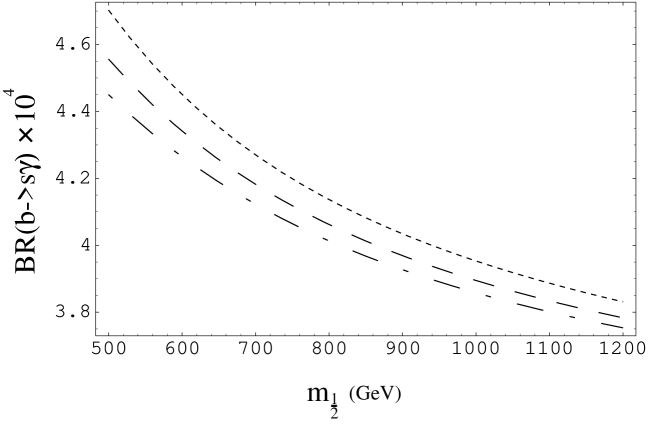
FIG. 1.: BR of $b\rightarrow s+\gamma$ is plotted as a function of the universal gaugino mass ($m_{1/2}$) for $\tan\beta=41$. The dotted line is for $\delta_{1}=$3, $\delta_{2}=$-0.9 and $m_{0}=600$ GeV. The dashed line is for $\delta_{1}=$2.5, $\delta_{2}=$-0.9 and $m_{0}=700$ GeV. The dash-dotted line is for $\delta_{1}=$2, $\delta_{2}=$-0.9 and $m_{0}=800$ GeV.

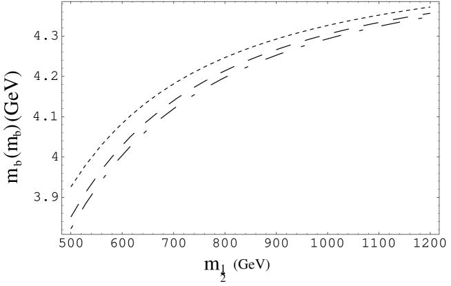
FIG. 2.: $m_{b}(m_{b})$is plotted as a function of the universal gaugino mass ($m_{1/2}$) for $\tan\beta=41$. The parameters for the curves are same as in fig. 1

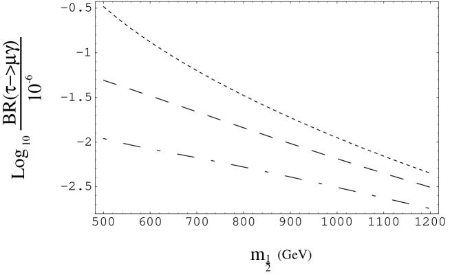
FIG. 3.: BR of $\tau\rightarrow\mu+\gamma$ is plotted as a function of the universal gaugino mass ($m_{1/2}$) for $\tan\beta=41$. The parameters for the curves are same as in fig. 1

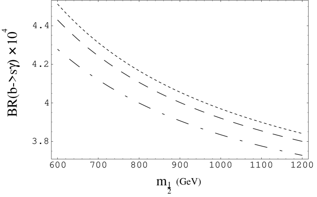
FIG. 4.: BR of $b\rightarrow s+\gamma$ is plotted as a function of the universal gaugino mass ($m_{1/2}$) for $\tan\beta=40$. The dotted line is for $\delta_{1}=$3, $\delta_{2}=$-0.9, $m_{0}=650$ GeV and $A_{0}=-550$ GeV. The dashed line is for $\delta_{1}=$3, $\delta_{2}=$-0.9, $m_{0}=700$ GeV and $A_{0}=-600$ GeV. The dash-dotted line is for $\delta_{1}=$2.5, $\delta_{2}=$-0.9, $m_{0}=800$ GeV and $A_{0}=-650$ GeV.

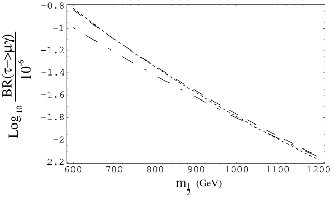
FIG. 5.: BR of $\tau\rightarrow\mu+\gamma$ is plotted as a function of the universal gaugino mass ($m_{1/2}$). The parameters for the curves are same as in fig. 4

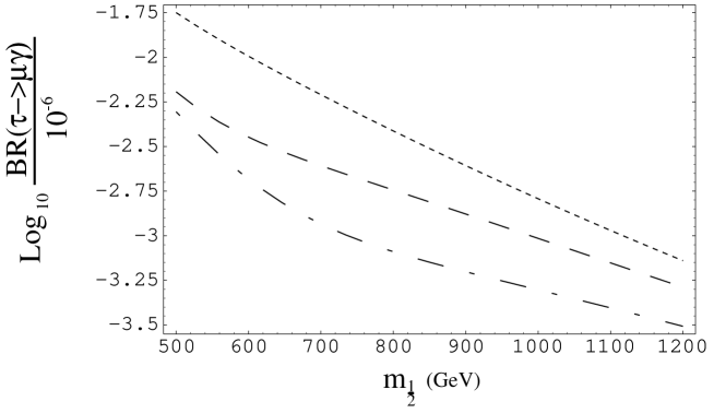
FIG. 6.: BR of $\tau\rightarrow\mu+\gamma$ is plotted as a function of the universal gaugino mass ($m_{1/2}$) for $\tan\beta=41$ in the case when doubly charged fields get decoupled at the left right scale. The dotted line is for $\delta_{1}=$3, $\delta_{2}=$-0.9 and $m_{0}=600$ GeV. The dashed line is for $\delta_{1}=$2.5, $\delta_{2}=$-0.9 and $m_{0}=700$ GeV. The dash-dotted line is for $\delta_{1}=$2, $\delta_{2}=$-0.9 and $m_{0}=800$ GeV.

REFERENCES

[1] R. Kuchimanchi and R. N. Mohapatra, Phys. Rev. D48, 4352
(1993); Phys. Rev. lett. 75, 3989 (1995); C. Aulakh, A. Melfo and G.
Senjanović, hep-ph/9707258;
Z. Chacko and R. N. Mohapatra, Phys. Rev. D 58, 015001 (1998);
C. Aulakh, K. Benakli and G. Senjanović, Phys. Rev. Lett.79, 2188
(1997). C. S. Aulakh, A. Melfo, A. Rasin and G. Senjanović, Phys. Rev.
D58, 115007 (1998).
[2] K. Huitu, J. Maalampi and M. Raidal, Nucl. Phys. B420,
449 (1994); Phys. Lett. B320, 60 (1994); B.Dutta and R. N. Mohapatra,
Phys. Rev. D 59, 015018 (1999); B. Dutta, D. Muller and R. N. Mohapatra,
hep-ph/9810443; G. Couture, M. Frank, H. Konig and
M. Pospelov, Eur.Phys. J. C7, 135 (1999).
[3] J. C. Pati and A. Salam, Phys. Rev. D 10, 275 (1974); R. N.
Mohapatra and J. C. Pati, Phys. Rev. D11, 566, 2558 (1975); G.
Senjanović and R. N. Mohapatra, Phys. Rev. D12, 1502 (1975).
[4] K. S. Babu, B. Dutta and R. N. Mohapatra, hep-ph/9812421.
[5] L. Hall, R. Rattazi and U. Sarid, LBL-33997 (1993); T. Blazek, S.
Pokorski and S. Raby, hep-ph/9504364.
[6] For discussions of up-down unification in other models, see D.
Chang, R. N. Mohapatra, P. B. Pal and J. C. Pati, Phys. Rev. Lett. 55,
2756 (1985); C. Hamzaoui and M. Pospelov, hep-ph/9803354.
[7] R. Barbieri, L. Hall and A. Strumia, Phys. Lett. B338,
212,(1994); Nucl. Phys. B445,219,(1995); N. G. Deshpande, B. Dutta
and E. Keith, Phys. Rev. D54,730,(1996).
[8] The Super-Kamiokande Collaboration, Phys Rev. Lett. 81,
1562 (1998); T. Kajita, hep-ex/9810001.
[9] L. Wolfenstein, Phys. Rev. D17, 2369 (1978); S.P.
Mikheyev and A.Y. Smirnov, Yad. Fiz. 42, 1441 (1985).
[10] N. Hata and P. Langacker,Phys. Rev. D56, 6107 (1997); P
Krastev and S. Petcov, Nucl. Phys. B449, 605 (1995).
[11] K. S. Babu, C. N. Leung and J. Pantaleone, Phys. Lett. B319, 191 (1993); P. H. Chankowski and Z. Pluciennik, Phys. Lett. B316, 312 (1993); N. Haba, Y. Matsui, N. Okamura and M. Sugiura,
hep-ph/9904292.
[12] M. Fukugita, T. Yanagida, Phys. Lett. 144B,386,(1984); For recent works, see M. Flanz, E. A. Pascos and U.
Sarkar, Phys. Lett. B 345, 248 (1995); L. Covi, E. Roulet and F.
Vissani, Phys. Lett. B 384, 169 (1996); E. Ma, S. Sarkar and U.
Sarkar, hep-ph/9812276; W. Buchmuller and M. Plumacher, hep-ph/9904310;
B. Brahmachari and M. Berger, hep-ph/9903406.
[13] T.V. Duong, B. Dutta and E. Keith, Phys. Lett. B378
128,(1996).
[14]V. Barger, M.S. Berger, P. Ohmann, Phys. Rev. D49,4908,(1994).
[15] R. Rattazzi and U. Sarid, Phys. Rev. D53, 1553 (1996).
[16] M. Carena, M. Olechowski and S. Pokorski, Nucl. Phys. B426
269, (1994).
[17] T. Blazek and S. Raby , hep-ph/9712257.
[18] M.S. Alam et.al (CLEO collab.), Phys. Rev. Lett. 74, 2885
(1995).
[19] Particle Data Group, European Physical Journal C 3,
288 (1998).
[20] See S. Gentile and M. Pohl, CERN-PPE/95-147 (1995) and
A. Weinstein and R. Stroynowski, CALT-68-1853 for reviews and prospects
in the -lepton decays.