BARI-TH/99-333

Radiative Leptonic $B_{c}$ Decays
P. Colangelo , F. De Fazio
Istituto Nazionale di Fisica Nucleare, Sezione di Bari, Italy

Abstract

We analyze the radiative leptonic $B_{c}$ decay mode: $B_{c}\to\ell\nu\gamma$ ($\ell=e,\mu$) using a QCD-inspired constituent quark model. The prediction: ${\cal B}(B_{c}\to\ell\nu\gamma)\simeq 3\times 10^{-5}$ confirms that this channel is experimentally promising in view of the large number of $B_{c}$ mesons which are expected to be produced at the future hadron facilities.

Recently, the CDF Collaboration at the Fermilab Tevatron has reported the observation of the $B_{c}$ meson, the lowest mass ${\bar{b}}c$ ($b{\bar{c}}$) bound state, through the semileptonic decay mode $B_{c}^{\pm}\to J/\psi\ell^{\pm}X$ [1]. The measured mass and lifetime of the meson are

$$M_{B_{c}} = 6.40\pm 0.39\;({\rm stat})\;\pm 0.13\;({\rm syst})\;{\rm GeV}$$ (1)

$$\tau(B_{c}) = 0.46^{+0.18}_{-0.16}\;({\rm stat})\pm 0.03\;({\rm syst})\;{\rm ps}\;\;\;.$$ (2)

The particular interest of this observation is related to the fact that the meson ground-state with open beauty and charm can decay only weakly, thus providing the rather unique opportunity of investigating weak decays in a heavy quarkonium-like system. Moreover, studying this meson, important information can be obtained, not only concerning fundamental parameters, such as, for example, the element $V_{cb}$ of the Cabibbo-Kobayashi-Maskawa mixing matrix, but also the strong dynamics responsible of the binding of the quarks inside the hadron. Understanding such dynamics is one of the most important issues in the analysis of heavy hadrons [2]. The observation of the $B_{c}$ meson at the Tevatron confirms that $B_{c}$ physics will gain an important role at the future hadron facilities, where a large production rate of such particles is expected; in particular, at the Large Hadron Collider (LHC), which will be operating at CERN, it is estimated that $4.5\times 10^{10}$ $B_{c}^{+}$ mesons will be produced per year for a machine luminosity of ${\cal L}=10^{34}$ cm^-2 sec^-1 at ${\sqrt{s}}=14$ TeV [3].

$B_{c}$ meson decays can be classified according to the mechanism inducing the processes at quark level. Neglecting Cabibbo-suppressed and penguin-induced transitions, such mechanisms are:

• the $b$-quark transition $b\to c\;W^{-}$, with the ${\bar{c}}$ quark having the role of spectator; the corresponding final states are of the kind $J/\psi\;\pi$, $J/\psi\;\ell\nu$;

• the charm quark transition ${\bar{c}}\to{\bar{s}}\;W^{-}$, with $b$ as spectator and possible final states $B_{s}\;\pi$, $B_{s}\;\ell\nu$, etc.;

• the annihilation modes ${\bar{c}}b\to W^{-}$.

The first two mechanisms are responsible of the largest part of the $B_{c}$ decay width [5, 6, 7]. In particular, the measurement (2) provides us with an indication that the dominant $B_{c}$ decay mechanism is the $c$-quark decay, which implies a $B_{c}$ lifetime in the range $\tau_{B_{c}}=(0.4-0.7)\;ps$ [7], whereas dominance of the $b-$quark decay mechanism would produce a longer lifetime: $\tau_{B_{c}}=(1.1-1.2)\;ps$ [6]. Various analyses of $B_{c}$ transitions induced by the two mechanisms are available in the literature [2]; for example, a QCD sum rule calculation of $B_{c}$ semileptonic decays suggested the dominance of the charm transition [8].

As far as the annihilation processes are concerned, the leptonic radiative decay mode $B_{c}\to\ell\nu\gamma$ and the leptonic decay without photon in the final state represent a minor fraction of the $B_{c}$ full width. Nevertheless, their analysis is of particular interest, both from the phenomenological and the theoretical point of view. From the phenomenological side, $B_{c}$ annihilation modes are governed by $V_{cb}$; therefore they are Cabibbo-enhanced with respect to the analogous $B_{u}$ decays, and represent new channels to access this matrix element. From the theoretical viewpoint, the purely leptonic and the radiative leptonic $B_{c}$ transitions are interesting since, in the nonrelativistic limit of the quark dynamics, both their rates can be expressed in terms of a single hadronic parameter, the $B_{c}$ leptonic decay constant $f_{B_{c}}$ [9, 10]. In this limit, a relation between the widths of the processes $B_{c}\to\ell\nu\gamma$ and $B_{c}\to\ell\nu$ can be worked out [9, 10]:

$$R_{\ell}={\Gamma(B_{c}\to\ell\nu\gamma)\over\Gamma(B_{c}\to\ell\nu)}\simeq 0.40\;r_{\ell}$$ (3)

with $\displaystyle{r_{\ell}={\alpha\over 4\pi}{m_{B_{c}}^{2}\over m_{\ell}^{2}}}$. Eq.(3) implies that the width of the radiative leptonic $B_{c}$ decay into muons is nearly equal to the purely leptonic width $\Gamma(B_{c}\to\mu\nu)$, whereas, in the case of electrons in the final state, the radiative leptonic mode is largely dominant.

Eq.(3) presents uncertainties coming from the used values of the charm and beauty quark masses. Moreover, there could be corrections if the quark dynamics in the $B_{c}$ meson deviates from the nonrelativistic regime, and the size of the corrections is useful for understanding the theoretical uncertainty affecting the ratio (3).

Corrections to the ratio (3) can be estimated by considering a model for the $B_{c}$ meson where relativistic effects in the constituent quark dynamics are, at least partially, taken into account; the present letter is devoted to such a study.

In order to analyze the decay mode $B_{c}\to\ell\nu\gamma$ ($\ell=e,\mu$), we follow the method adopted in ref.[11] to investigate the analogous $B_{u}$ transition. Let us consider the process

$$B_{c}^{-}(p)\to\ell^{-}(p_{1})\;{\bar{\nu}}(p_{2})\;\gamma(k,\epsilon)$$ (4)

whose amplitude can be written as

$${\cal A}(B_{c}\to\ell{\nu}\gamma)={G_{F}\over\sqrt{2}}V_{cb}\;\;\epsilon^{*\nu}\;\;\big{(}L^{\mu}\cdot\Pi_{\mu\nu}-ief_{B_{c}}p^{\mu}\tilde{L}_{\mu\nu}\big{)}\hskip 10.0pt,$$ (5)

with $G_{F}$ the Fermi constant and $\epsilon$ the photon polarization vector. The current $L^{\mu}={\bar{\ell}}(p_{1})\gamma^{\mu}(1-\gamma_{5})\nu(p_{2})$ represents the weak leptonic current in (4). The hadronic function $\Pi_{\mu\nu}(p,k)$ is the correlator

$$\Pi_{\mu\nu}(p,k)=i\;\int d^{4}xe^{iq\cdot x}<0|T[J_{\mu}(x)V_{\nu}(0)]|B_{c}(p)>\hskip 3.0pt$$ (6)

with $J_{\mu}(x)={\bar{c}}(x)\gamma_{\mu}(1-\gamma_{5})b(x)$ the weak hadronic current governing (4) and $V_{\nu}$ given by $V_{\nu}(0)=e[Q_{c}\;{\bar{c}}(0)\gamma_{\nu}c(0)+Q_{b}\;{\bar{b}}(0)\gamma_{\nu}b(0)]$, $eQ_{c}$ and $eQ_{b}$ being the charm and beauty quark electric charges. The momentum $q$ is defined as $q=p_{1}+p_{2}$. Therefore, the first term in (5) correspond to the photon emitted from the meson, and the second term represents the contribution of the photon emitted by the charged lepton leg. Notice that the $B_{c}$ leptonic constant $f_{B_{c}}$ is defined by the matrix element

$$<0|\bar{c}\gamma_{\mu}\gamma_{5}b|B_{c}(p)>=if_{B_{c}}p_{\mu}$$ (7)

and that $\tilde{L}_{\mu\nu}$ reads

$$\tilde{L}_{\mu\nu}={\bar{\ell}}(p_{1})\gamma^{\nu}{1\over{\not\!p\,}_{1}+{\not\!k\,}-m_{l}}\gamma^{\mu}(1-\gamma_{5})\nu(p_{2})\;\;.$$ (8)

The hadronic function $\Pi_{\mu\nu}(p,k)$ can be expanded in independent Lorentz structures

$$\Pi_{\mu\nu}(p\cdot k)=\alpha\;p_{\mu}p_{\nu}+\beta\;k_{\mu}k_{\nu}+\zeta\;k_{\mu}p_{\nu}+\delta\;p_{\mu}k_{\nu}+\xi\;g_{\mu\nu}+i\eta\epsilon_{\mu\nu\rho\sigma}p^{\rho}k^{\sigma}\;\,\;$$ (9)

(with the invariant functions $\alpha,\dots\eta$ depending on $p\cdot k$) so that the requirement of gauge invariance for the amplitude (5) implies the condition:

$$(\alpha+\zeta)(p\cdot k)+\xi-ief_{B_{c}}=0\;\;\;.$$ (10)

We shall see in the following that this condition is satisfied in our calculation.

The final expression of the amplitude, eq.(5),

$${\cal A}(B_{c}\to\ell{\nu}\gamma)={G_{F}\over\sqrt{2}}V_{cb}\;\;\epsilon^{*\nu}\;L^{\mu}[(\alpha+\zeta)\;(k_{\mu}p_{\nu}-p\cdot k\;g_{\mu\nu})+i\;\eta\;\epsilon_{\mu\nu\rho\sigma}p^{\rho}k^{\sigma}]\;\epsilon^{*\nu}\;\;\;,$$ (11)

is given in terms of the form factors $\eta$ and $\zeta+\alpha$, related to the vector and the axial vector weak current contributions to the process (4), respectively.

In order to compute the invariant functions in (11) we employ the costituent quark model developed in ref.[12] to describe the static properties of mesons containing heavy quarks. In the correlator (6) we write the state of the pseudoscalar $(b{\bar{c}})$ meson at rest in terms of a wave-function $\psi_{B_{c}}$ and of quark and antiquark creation operators:

$$|B_{c}^{-}>=i{\delta_{\alpha\beta}\over\sqrt{3}}{\delta_{rs}\over\sqrt{2}}\int d\vec{k}\;\psi_{B_{c}}(\vec{k})\;b^{{\dagger}}(\vec{k},r,\alpha)\;c^{{\dagger}}(-\vec{k},s,\beta)|0>\hskip 5.0pt;$$ (12)

$\alpha$ and $\beta$ are colour indices, $r$ and $s$ spin indices; the operator $b^{{\dagger}}$ creates a $b$ quark with momentum ${\vec{k}}$, while $c^{{\dagger}}$ creates a charm antiquark with momentum $-\vec{k}$. The wave-function $\psi_{B_{c}}$, describing the quark momentum distribution in the meson, is obtained as a solution of the Salpeter equation

$$\Big{\{}\sqrt{\vec{k}^{2}+m_{b}^{2}}+\sqrt{\vec{k}^{2}+m_{c}^{2}}-m_{B_{c}}\Big{\}}\psi_{B_{c}}(\vec{k})+\int d\vec{k^{\prime}}\;V(\vec{k},\vec{k^{\prime}})\;\psi_{B_{c}}(\vec{k^{\prime}})=0$$ (13)

stemming from the quark-antiquark Bethe-Salpeter equation, in the approximation of an istantaneous interaction represented by the interquark potential $V$. Within the model in [12], $V$ is chosen as the Richardson potential [13], which reads in the $r-$space:

$$V(r)={8\pi\over 33-2n_{f}}\Lambda\Big{[}\Lambda r-{f(\Lambda r)\over\Lambda r}\Big{]}\;\;\;,$$ (14)

with $\Lambda$ a parameter, $n_{f}$ the number of active flavours, and the function $f(t)$ given by:

$$f(t)={4\over\pi}\int_{0}^{\infty}dq{sin(qt)\over q}\Big{[}{1\over ln(1+q^{2})}-{1\over q^{2}}\Big{]}\;.$$ (15)

The linear increase at large distances of the potential in (14) provides QCD confinement; at short distances the potential behaves as $-{\alpha_{s}(r)\over r}$, with $\alpha_{s}(r)$ logarithmically decreasing with the distance $r$, thus reproducing the asymptotic freedom property of QCD. A smearing procedure at short-distances is also adopted, to account for effects of the relativistic kinematics [12]. Finally, spin interaction effects are neglected since in the case of heavy mesons the chromomagnetic coupling is of order of the inverse heavy quark masses.

The interest for eq.(13) is that relativistic effects are taken into account at least in the quark kinematics. Therefore, the same wave-equation can be used to study heavy-light as well as heavy-heavy quark systems, and one case can be obtained from the other one by continuously varying a parameter, the $u(c)$ quark mass. From the analysis of the solutions, a comparison between the two cases, the heavy-light and the heavy-heavy quark meson systems, can be meaningfully performed.

Eq.(13) can be solved by numerical methods, as described in [12], fixing the masses $m_{c}$ and $m_{b}$ of the constituent quarks, together with the parameter $\Lambda$, in such a way that the charmonium and bottomomium spectra are reproduced. The chosen values for the parameters are: $m_{b}=4.89$ GeV and $m_{c}=1.452$ GeV, with $\Lambda=397$ MeV [12]. A fit of the heavy-light meson masses also fixes the values of the constituent light-quark masses: $m_{u}=m_{d}=38$ MeV [12]. For the $b\bar{c}$ system all the input parameters required in (13) are fixed from the analysis of other channels, and the predictions do not depend on new external quantities. The numerical solution of (13) produces spectrum of the $b\bar{c}$ bound states; the predicted masses of the first three radial $S-$wave resonances are reported in Table 1.

radial number	mass (GeV)	leptonic constant (MeV)
$0$	6.28	432
$1$	6.80	313
$2$	7.16	265

Table 1: Spectrum and leptonic constants of the pseudoscalar $b\bar{c}$ mesons.

The spectrum in Table 1 agrees with other theoretical determinations based on constituent quark models [14]. As for QCD sum rule and lattice QCD results, in [8] the value $m_{B_{c}}=6.35$ GeV was found using two-point function QCD sum rules, whereas a recent lattice QCD analysis predicts: $m_{B_{c}}=6.388\pm 9\pm 98\pm 15$ GeV, with the larger error related to the quenched approximation [15]. Within the errors, the mass of the $B_{c}$ meson in Table 1 agrees with the CDF measurement reported in eq.(1).

Also the wave-function $\psi_{B_{c}}$ can be obtained by solving eq.(13). We use the covariant normalization:

$${1\over(2\pi)^{3}}\int d\vec{k}|\psi_{B_{c}}(\vec{k})|^{2}=2m_{B_{c}}\hskip 3.0pt$$ (16)

and define, in the $B_{c}$ meson rest-frame, the reduced wave-function $u_{B_{c}}(k)$ ($k=|{\vec{k}}|$):

$$u_{B_{c}}(k)={k\;\psi_{B_{c}}(k)\over\sqrt{2}\pi}\hskip 3.0pt$$ (17)

which is normalized as: $\int_{0}^{\infty}dk|u_{B_{c}}(k)|^{2}=2m_{B_{c}}$. In fig.1 the $B_{c}$ meson wave-function $u_{B_{c}}(k)$ is depicted, together with the function $u_{B_{u}}$ of the $B_{u}$ meson.

Figure 1: $B_{c}$ meson wave-function (continuous line). The wave-function of the $B_{u}$ meson is also depicted (dashed line).

The meson wave-functions, together with the predictions of the spectrum of the bound states, are the main results of the model; they allow us to calculate hadronic quantities such as the leptonic decay constants and the strong couplings to light mesons [12, 16]. In particular, using $u_{B_{c}}(k)$ depicted in fig.1, we can infer the size of the deviation from the nonrelativistic limit in the Salpeter equation (13). As a matter of fact, the average squared quark momentum $<k^{2}>$ turns out to be $<k^{2}>=0.95$ GeV², and the ratios $<k^{2}>/m_{c}^{2}=0.43$ and $<k^{2}>/m_{b}^{2}=0.04$. In the case of the $B_{u}$ meson, the average squared quark momentum $<k^{2}>$ is $<k^{2}>=0.47$ GeV², to be compared to $m_{u}^{2}=1.4\times 10^{-3}$ GeV². Therefore, in the case of $B_{c}$ mesons, deviations from the nonrelativistic limit, although small, are not negligible, mainly due to term related to the charm quark.

Before coming to the analysis of the radiative leptonic $B_{c}$ decay and to the calculation of the ratio (3), let us evaluate the leptonic constants $f_{B_{c}^{n}}$ of the $S$-wave excitations, defined by matrix elements analogous to (7). The numerical results, obtained from the eigenfunctions of eq.(13), are reported in Table 1. Few comments are in order. The value of $f_{B_{c}}$ in Table 1 is compatible, within the theoretical errors, with the result $f_{B_{c}}=360\pm 60$ MeV obtained from QCD sum rules [8] (the uncertainty related to the input parameters of the potential model is estimated of $\pm 15\%$ for the leptonic constants [12]). On the other hand, the leptonic constants in Table 1 are smaller than the outcome of several constituent quark models considered in [14], based on a purely nonrelativistic description of the $b\bar{c}$ system. Notice that the decreasing values of $f_{B_{c}^{n}}$, for increasing radial number $n$, is due to the nodes of the wave-functions of the radial excitations. Finally, the $B_{c}$ leptonic constant turns out to be compatible with a lattice NRQCD determination [17].

Let us now consider the correlator (6). Writing the state $|B_{c}>$ as in (12) and expanding the T-product according to the Wick theorem, we can express the product of the two currents $J_{\mu}(x)V_{\nu}(0)$ in terms of quark creation and annihilation operators; then, exploiting the anticommutation relations between such operators, we can derive an expression for $\Pi_{\mu\nu}$ in terms of the $B_{c}$ wave function, $u_{B_{c}}$, which is analogous to the expression reported in [11] for the $B_{u}$ decay.

It is useful to relate the invariant functions in (9) to the various components of the hadronic tenson $\Pi_{\mu\nu}$. In the $B_{c}$ rest-frame $p=(m_{B_{c}},{\vec{0}})$ and choosing $k^{\mu}=(k^{0},0,0,k^{0})$ one gets from eq.(6):

$$\zeta(k^{0}) = {1\over m_{B_{c}}k^{0}}(\Pi_{30}-\Pi_{33}+\Pi_{11})$$

$$\alpha(k^{0}) = {1\over m_{B_{c}}^{2}}(\Pi_{00}+\Pi_{33}-\Pi_{30}-\Pi_{03})$$

$$\eta(k^{0}) = -i{1\over m_{B_{c}}k^{0}}\Pi_{12}(k^{0})\hskip 10.0pt.$$ (18)

Therefore, the condition (10) ensuring gauge invariance can be written as

$$ief_{B_{c}}={k^{0}\over m_{B_{c}}}\big{(}\Pi_{00}+\Pi_{33}-\Pi_{30}-\Pi_{03}\big{)}+\Pi_{30}-\Pi_{33}\;\;\;,$$ (19)

a condition that must be checked in our analysis. The explicit calculation, using the expression of $\Pi_{\mu\nu}$ in terms of the meson wave-function [11], shows that eq.(19) is verified provided that the leptonic constant $f_{B_{c}}$ is given by

$$f_{B_{c}}=\sqrt{3}{1\over 2\pi m_{B_{c}}}\int_{0}^{\infty}dk^{\prime}\;k^{\prime}\;u_{B_{c}}(k^{\prime})\big{[}{(E_{b}+m_{b})(E_{c}+m_{c})\over E_{b}E_{c}}\big{]}^{1\over 2}\Big{[}1-{k^{\prime 2}\over(E_{b}+m_{b})(E_{c}+m_{c})}\Big{]}$$ (20)

with $E_{b,c}=\sqrt{k^{\prime 2}+m_{b,c}^{2}}$. Indeed, eq.(20) is the expression for $f_{B_{c}}$ obtained in the framework of the constituent quark model [12], hence the gauge invariance property of the amplitude (5) is preserved in our calculation.

Having checked the property of gauge invariance, we can simply compute the decay width of the mode (4) and the photon energy distribution. Notice that we compute the photon energy spectrum for a photon energy larger than $100$ MeV, which represents the photon energy resolution we assume in our analysis.

The expression for the width of the decay (4), considering massless leptons in the final state ($m_{\ell}\simeq 0$), is

$$\Gamma(B_{c}\to\ell{\nu}\gamma)={G_{F}^{2}|V_{cb}|^{2}\over 3(2\pi)^{3}}\int_{0}^{m_{B_{c}}/2}dk^{0}k^{0}(m_{B_{c}}-2k^{0})[|\Pi_{11}+ief_{B_{c}}|^{2}+|\Pi_{12}|^{2}]\hskip 3.0pt.$$ (21)

Using the data in (1),(2), together with $V_{cb}=0.04$, we predict:

$$\Gamma(B_{c}\to\ell\nu\gamma)=4\;10^{-16}GeV\hskip 14.22636pt,\hskip 14.22636pt{\cal B}(B_{c}\to\ell\nu\gamma)=3\;10^{-5}\;.$$ (22)

The energy spectrum of the photon, computed using eq.(21), is depicted in fig.2; it looks symmetric with respect to the point $E_{\gamma}=m_{B_{c}}/4$, as observed also in [9, 10, 19].

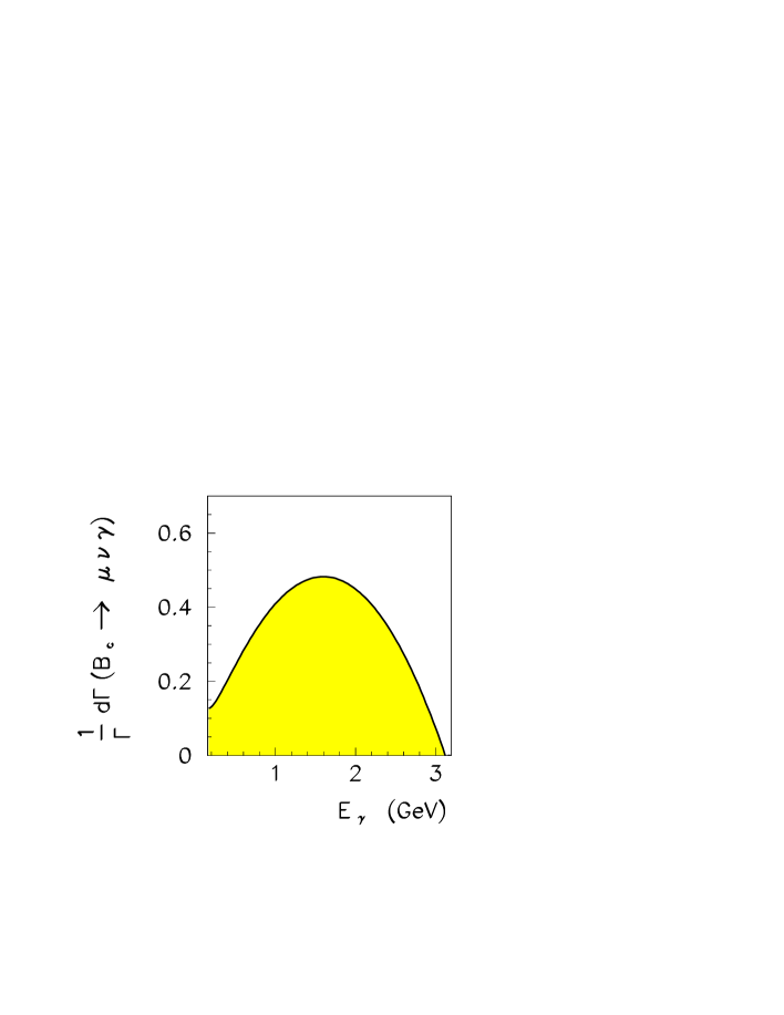
Figure 2: Photon energy spectrum in the decay (4)

.

The result (22) confirms that the rate of the radiative leptonic $B_{c}$ decays into muons (and electrons) is sizeable, and could be accessed at the future hadronic machines, such as LHC.

Let us now consider the ratio (3). In order to determine it, we need the width of the purely leptonic $B_{c}$ decay into electrons and muons, given by

$$\Gamma(B_{c}\to\ell\nu)={G_{F}^{2}\over 8\pi}|V_{cb}|^{2}f_{B_{c}}^{2}\Bigg{(}{m_{\ell}\over m_{B_{c}}}\Bigg{)}^{2}m_{B_{c}}^{3}\Bigg{(}1-{m_{\ell}^{2}\over m_{B_{c}}^{2}}\Bigg{)}^{2}\hskip 3.0pt,$$ (23)

which depends on $f_{B_{c}}$. Using the value in Table 1 we obtain:

$$\Gamma(B_{c}\to\mu\nu)=1.1\;10^{-16}\;GeV\hskip 14.22636pt,\hskip 14.22636pt{\cal B}(B_{c}\to\mu\nu)=7.8\;10^{-5}\;\;\;,$$ (24)

corresponding to $\displaystyle R_{\mu}={\Gamma(B_{c}\to\mu\nu\gamma)\over\Gamma(B_{c}\to\mu\nu)}\simeq 0.4$. This result must be compared to the value $R_{\mu}\simeq 0.8$ obtained using eq.(3) [9, 10], and suggests that the corrections to the nonrelativistic limit, although small, play a role in modifying the prediction (3). In any case, the widths of the radiative leptonic and the purely leptonic $B_{c}$ transitions are still comparable, a result which is very different from the case of radiative leptonic $B_{u}$ decays, which are enhanced with respect to the purely leptonic decay modes into muons and electrons. In that latter case, the helicity suppression, displayed by the factor $\big{(}{m_{\ell}\over m_{B_{q}}}\big{)}^{2}$ in (23) and producing very small decay rates, is efficiently avoided by the presence of the photon in the final state also in the case of muons, so that the branching fraction of the radiative leptonic $B_{u}$ modes into muons turns out to be enhanced by one order of magnitude with respect to the purely muon leptonic decay [11, 20].

As for the decay into electrons, we predict ${\cal B}(B_{c}\to e\nu_{e})\simeq 2\times 10^{-9}$.

The decay mode $B_{c}\to\ell\nu\gamma$ has been investigated, as mentioned above, in the framework of the nonrelativistic quark model (NRQM) [9, 10], and also using the light front quark model (LFQM) [18] and light-cone QCD sum rules (LCSR) [19]. In Table 2 we report the various predictions, obtained using the value of $f_{B_{c}}$ reported in Table 1. We also report the estimates of the ratio

$$r={N_{B_{u}}\over N_{B_{c}}}={{\cal B}(B_{u}\to\ell\nu\gamma)\over{\cal B}(B_{c}\to\ell\nu\gamma)}$$ (25)

which represents the relative fraction of the final state $\ell\nu\gamma$ coming from the different sources $B_{u}$ and $B_{c}$.

${\cal B}(B_{c}\to\ell\nu\gamma)$	r	method	ref.
$3\times 10^{-5}$	$0.03$	Rel. QM	This paper
$6\times 10^{-5}$		NRQCD	[10]
$6\times 10^{-5}$	$0.06-0.1$	NRQM	[9]
$2\times 10^{-5}$		LFQM	[18]
$2\times 10^{-5}$	$0.1$	LCSR	[19]

Table 2: Results for ${\cal B}(B_{c}\to\ell\nu\gamma)$ by different approaches.

Our small result: $r=0.03$ means that a large number of $\ell\nu\gamma$ final states should come from $B_{c}$ decays; the actual fraction of radiative leptonic final states can be obtained by multiplying eq.(25) by the probabilities of producing $B_{u}$ and $B_{c}$ mesons from $b$ quarks.

Let us conclude our analysis, based on a QCD-inspired relativistic constituent quark model, observing that the quark dynamics inside the $B_{c}$ meson could modify the prediction (3). Therefore, the range $[0.4-0.8]$ for the ratio (3) can be interpreted as the theoretical uncertainty for this quantity. The measurement of the radiative leptonic $B_{c}$ decay rate, together with the purely leptonic rate, although challenging from the experimental viewpoint, is one of the expected results in the LHC era.

Acknowledgments
We thank G. Nardulli and N. Paver for discussions.

References

- [1] CDF Collab., F. Abe et al., Phys. Rev. Lett. 81 (1998) 2432; Phys. Rev. D 58 (1998) 112004.
- [2] For a review of the properties and decays of see: S.S. Gershtein et al., hep-ph/9803433, hep-ph/9504319.
- [3] K. Cheung, Phys. Rev. Lett. 71 (1993) 3413.
- [4] K. Kolodziej, A. Leike and R. Rückl, Phys. Lett. B 355 (1995) 337 C.H. Chang, Y.Q. Chen, G.P. Han and H.T. Jiang, Phys. Lett. B 364 (1995) 78; C.H. Chang, Y.Q. Chen, and R.J. Oakes, Phys. Rev. D 54 (1996) 4344.; A.V. Berezhnoy, V.V. Kiselev, A.K. Likhoded and A.I. Onishchenko, Yad. Fiz. 60 (1997) 1886.
- [5] M. Lusignoli and M. Masetti, Z. Phys. C 51 (1991) 549.
- [6] C. Quigg, in Proceedings of the Workshop on B Physics at Hadron Accelerators, Snowmass, Colorado 1993, edited by P. McBride and C.S. Mishra, pag.439.
- [7] M. Beneke and G. Buchalla, Phys. Rev. D 53 (1996) 4991.
- [8] P. Colangelo, G. Nardulli and N. Paver, Z. Phys. C 57 (1993) 43.
- [9] C.H. Chang, J.P. Cheng and C.D. Lü, Phys. Lett. B 425 (1998) 166.
- [10] G. Chiladze, A.F. Falk and A.A. Petrov, Phys. Rev. D 60 (1999) 034011.
- [11] P. Colangelo, F. De Fazio and G. Nardulli, Phys. Lett. B 386 (1996) 328.
- [12] P. Cea, P. Colangelo, L. Cosmai and G. Nardulli, Phys. Lett. B 206 (1988) 691; P. Colangelo, G. Nardulli and M. Pietroni, Phys. Rev. D 43 (1991) 3002.
- [13] J. L. Richardson, Phys. Lett. B 82 (1979) 272.
- [14] W. Kwong and J. Rosner, Phys. Rev. D 44 (1991) 212; E. Eichten and C. Quigg, Phys. Rev. D 49 (1994) 5845; S.S. Gershtein et al., Phys. Rev. D 51 (1995) 3613; L.P. Fulcher, Phys. Rev. D 60 (1999) 074006 and references therein.
- [15] H.P. Shanahan, P.Boyle, C.T.H. Davies and H. Newton, UKQCD Collab., Phys. Lett. B 453 (1999) 289.
- [16] P. Colangelo, F. De Fazio and G. Nardulli, Phys. Lett. B 334 (1994) 175.
- [17] B.D. Jones and R.M. Woloshyn, Phys. Rev. D 60 (1999) 014502.
- [18] C.C. Lih, C.Q. Geng and W.M. Zhang, Phys. Rev. D 59, 114002 (1999).
- [19] T.M. Aliev and M. Savci, Phys. Lett. B 434 (1998) 358; J. Phys. G 25 (1999) 1205.
- [20] G. Burdman, T. Goldman and D. Wyler, Phys. Rev. D 51 (1995) 111; D. Atwood, G. Eilam and A. Soni, Mod. Phys. Lett. A 11 (1996) 1061; G.Eilam, I. Halperin and R.R.Mendel, Phys. Lett. B 361 (1995) 137; P. Colangelo, F. De Fazio and G. Nardulli, Phys. Lett. B 372 (1996) 331.