Abstract

Two photon decay widths of the $J^{P}=O^{+}$ scalar mesons $a_{0}(980)$, $f_{0}(980)$, $f_{0}(1370)$ and $\chi_{c0}$ are calculated in a covariant model which is characterized by the quark - antiquark structure. Previously such models were used to calculate current form factors. Here a different application is tried. A simple version of the model uses adjusted nonrelativistic model parameters with small quark masses. The results seem to prefer nonideal mixing of $f_{0}(980)$ and $f_{0}(1370)$. The calculated decay rate of $\chi_{c0}$ agrees with the experimental results.

Short title: Two photon decays of scalar mesons

PACS Nos.: 12.39.Ki, 12.39.Hg, 13.20.-v, 13.25.-k

1 Introduction

The scalar mesons appearing around 1 $GeV$ mass scale seems to be least understood among spin zero mesons. The experimental data[1], on strong decays of $a_{0}(980)$, $f_{0}(980)$ and $f_{0}(1370)$ do not lead to the final understanding of the real structure of these mesons [2]$-$[17]. Ideas exists that these states are $K\bar{K}$ molecules [2]$-$[7]. There is a suggestion that $a_{0}(980)$ has a four-quark structure with the strange quarks ($s\bar{s}$) contribution[16], based on the analyses of the $\phi\to\gamma a_{0}(980)\to\gamma\eta\pi$[17]. Such uncertainties suggest further investigation, which were concentrated on $2\gamma$ decays of $a_{0}(980)$, $f_{0}(980)$, $f_{0}(1370)$ and $\chi_{c0}$ mesons. The aim was to explain the experimental decay widths and at the same time to reproduce the measured masses.

The relativistic quark model is used to correlate various data and to establish the connection between masses and decay widths.

For that purpose one employs the covariant model [18, 19] which includes the heavy - quark symmetry. As shown in the following section the model and the calculations are both covariant and gauge invariant. This model is a covariant generalization [18, 19] of the well known ISGW model [20]. However, here the usage of small quark masses is investigated, which means the avoidance of the weak binding limit approximation in its strictest sense [20]. That might better mimick the real quark fields which should appear in the photon emitting quark loop (Fig. 1) in the first order of QED/QCD expansion. In a very simplified version of that model, which is employed here, only the quark momentum distribution parameter $\beta$ and the model quark masses appear. All parameters are correlated and compared with the nonrelativistic choices[20, 21, 22] The quark masses,were treated as fitting parameters in a limited sense. Suitable values, allowed within the experimental uncertainty in current quark masses [1], were selected. That parameterization is expected to lead to a reasonable reproduction of meson masses. No additional fitting was allowed when widths were calculated. In that way one can reproduce the measured $\Gamma(2\gamma)$ reasonably well and make the prediction for the $f_{0}(1370)$ $2\gamma$ decay.

All results are based on the valent quark $q\overline{q}$ structure, which is characteristic of the model. The importance of $q\overline{q}$ structure has often been mentioned [7]$-$[14]. Our basic loop diagrams, Fig. 1 below, correspond closely to the quark loop diagrams shown in Fig. 1 of Ref.(10). Thus it is not surprising that our results, following from the somewhat more complicated diagrams, depends strongly on quark masses.

Moreover our model contains the sea component constrained by the requirement of general Lorentz covariance, valid in an frame [18, 19]. In that way, indirectly, some other QCD structures, as discussed earlier [18, 19], enter into our description.

Predictions based on our simplified model version test how well, or how badly the model mimicks the real QED/QCD world. The quarkonium approximation [20] is investigated here in the circumstances which are different from the usual form factors related problems[18, 20].

The results depend also on the quark flavor structure of the scalar mesons. They do distinguish among various propose $u\overline{u},d\overline{d}$ and $s\overline{s}$ mixing[13, 14] in $f_{0}$ mesons.We investigate only lower laying states without entering into discussion of the states as $a_{0}(1450)$ which would require to include the higher order terms of our model.

2 Brief description of the model

A scalar meson $H$ with the four-momentum $P$ and the mass $M$ is covariantly represented [18, 19] by

$$|H(E,\vec{P},M)\big{>}=\frac{N(\vec{P})}{(2\pi)^{3}}\sum_{c,s_{1},s_{2}}\ \ \sum_{f}C_{f}\ \ \int\ \big{[}4m_{1}m_{2}\big{]}\ d^{4}p\ \delta(p^{2}-m^{2}_{1})\ \Theta(e)$$

$$\cdot d^{4}q\ \delta(q^{2}-m^{2}_{2})\ \Theta(\epsilon)\ d^{4}K\ F(K)\ \delta^{(4)}(p+q+K-P)\ \Theta(E)\ \phi_{f}(l_{\perp})$$ (2.1)

$$\cdot\overline{u}_{f,s_{1}}^{c}(\vec{p})v^{c}_{f,s_{2}}(\vec{q})\ \ d^{+}_{f}(\vec{q},c,s_{2})b^{+}_{f}(\vec{p},c,s_{1})|0\big{>}$$

Here $m_{i}$ are quark masses and $f$ stands for quark flavor. The quark wave function is

$$\phi_{f}(l^{\mu}_{\bot})=\frac{1}{(1-\frac{l_{\bot}^{2}}{4\beta_{f,H}^{2}})^{2}}$$ (2.2)

$$l^{\mu}_{\bot}(P)=l^{\mu}-\frac{P^{\mu}(P\cdot l)}{M^{2}}$$

with $l^{\mu}=(p-q)^{\mu}/2$, $p^{\mu}=(e,\vec{p})$ and $q^{\mu}=(\epsilon,\vec{q})$. The fitting parameter $\beta_{f,H}\ \ (f=u,d,s,c)$ is fixed by fitting the meson mass as described below. The dipole form (2.2) was found to be a better choice than the exponential form used earlier [18, 19]. (See also some remarks in Appendix.) Coefficient $C_{f}$ indicates the flavor content of a particular meson (For example, see below formula (3.14), where for $f_{0}(980)\ \ C_{u}=cos(\theta)/\sqrt{2}$).

The symbols $\overline{u},v,d^{+},b^{+}$ correspond to valence quarks while the sea function has a general form

$$F(K)=\delta^{(4)}\big{[}K^{\mu}-\frac{P^{\mu}}{M}\frac{P^{\nu}\big{(}P-p-q\big{)}_{\nu}}{M}\big{]}\ \varphi(K).$$ (2.3)

For simplicity we set

$$\varphi(K)=1.$$ (2.4)

The complex looking Dirac function in (2.3) simplifies the model structure easing all formal manipulations. One could produce a somewhat more complicated model, without that Dirac function. Additional parameter(s) in the sea model function would lead to a richer and more flexible model [19]. Thus the choice (2.4) correspond to a minimalistic model version.

The scalar meson state (2.1) is normalized so that the matrix element of the vector current $V^{\mu}$ would be, for example,

$$\langle H(\vec{P}_{f})|V^{\mu}|H(\vec{P}_{i})\rangle=\frac{1}{(2\pi)^{3}}F_{+}(Q^{2})(P_{f}+P_{i})^{\mu}+\cdots$$ (2.5)

with $Q^{\mu}=(P_{f}-P_{i})^{\mu}$, $F_{+}(Q^{2}=0)=1$. The normalization (2.5) insures that the vector current, and thus charge, is conserved. This requirement is equivalent to the condition

$$\langle H(E,\vec{P},M)|H(E,\vec{P},M)\rangle=2E=$$

$$=\frac{N(\vec{P})^{2}}{(2\pi)^{6}}\sum_{c,s_{1},s_{2}}\sum_{c^{\prime},s^{\prime}_{1},s^{\prime}_{2}}\sum_{f,f^{\prime}}C_{f}C_{f^{\prime}}\cdot\int d^{3}p\frac{m_{1}m_{2}}{e}\frac{M}{E}\frac{\phi_{f}(l_{\bot})}{q_{\parallel}}d^{3}p^{\prime}\frac{m_{1}m_{2}}{e^{\prime}}\frac{M}{E}\frac{\phi_{f^{\prime}}(l^{\prime}_{\bot})}{q^{\prime}_{\parallel}}$$

$$\cdot[\overline{v}_{f^{\prime},c^{\prime},s^{\prime}_{2}}(\vec{q^{\prime}})u_{f^{\prime},c^{\prime},s^{\prime}_{1}}(\vec{p^{\prime}})\overline{u}_{f,c,s_{1}}(\vec{p})v_{f,c,s_{2}}(\vec{q})]\cdot$$

$$\cdot\big{<}0|b_{f^{\prime}}(\vec{p^{\prime}},c^{\prime},s^{\prime}_{1})d_{f^{\prime}}(\vec{q^{\prime}},c^{\prime},s^{\prime}_{2})d^{+}_{f}(\vec{q},c,s_{2})b^{+}_{f}(\vec{p},c,s_{1})|0\big{>}\big{|}_{\vec{q}=T_{1},\ \ \vec{q^{\prime}}=T_{1}^{\prime}}$$ (2.6)

Here

$$T_{1}=-\vec{p}+\frac{\vec{P}}{M}(p_{\parallel})T$$

$$T=1+\frac{\sqrt{m^{2}_{2}-m^{2}_{1}+p^{2}_{\parallel}}}{p_{\parallel}}\ \ \ ;\ \ \ \ \ p_{\parallel}=\frac{P\cdot p}{M}\ \ \ ;\ \ \ \ \ q_{\parallel}=\frac{P\cdot q}{M}$$ (2.7)

After a lengthy but straightforward manipulation, one find

$$N(\vec{P})=\frac{E}{M}N(0)$$

$$\langle H(E,\vec{P},M)|H(E,\vec{P},M)\rangle=2E=3N(0)^{2}\sum_{f}C_{f}^{2}\int d^{3}p\ \frac{\epsilon}{e}\ {\big{(}}\frac{\phi_{f}(l_{\bot})}{q_{\parallel}}{\big{)}}^{2}\ (pq-m_{1}m_{2})$$ (2.8)

¿From (2.8) $N(0)$ can be calculated numerically.

The matrix element of the conserved vector current $V^{\mu}$ has to vanish when current acts on the scalar meson state, i.e.

$$\langle 0|V^{\mu}|H(E,\vec{P},M)\rangle\equiv 0$$ (2.9)

The model states (2.1) are consistent with this very general requirement. Some additional details are shown in the Appendix.

So far the model is closely related to ISGW model [20]. In the nonrelativistic limit and in the weak binding approximation it goes exactly in the ISGW form[18, 19]. However the weak binding approximation means that the quark masses and the quark energies are approximately equal [20]. In the present application, the model quark fields enter a loop (Fig. 1) which constitutes the lowest QED approximation. The QCD corrections are modeled by the functions (2.2) and (2.3). One can try to mimick the real QED/QCD world by retaining small (current) quark masses in the model. Then the meson mass should be equal to a sum (weighted by the sea influence) of average model quark energies. In the model determined by (2.2) and (2.4) this i

$$M=\frac{3N(0)^{2}}{2E}\sum_{f}C_{f}^{2}\int d^{3}p\ (\frac{\phi_{f}(l_{\bot})}{q_{\parallel}})^{2}\ \frac{p\cdot q-m_{1}m_{2}}{e/\epsilon}(p_{\parallel}+q_{\parallel})|_{\vec{q}=-\vec{p}+\frac{\vec{P}}{M}(p_{\parallel})T}$$ (2.10)

As discussed in the Appendix this simple form holds in the minimalistic model version (2.4). The wave function $\phi_{p}$ can be connected with the usual potential^17,19,20 as shown in Appendix. In the nonrelativistic, weak binding limit (WBL) (2.10) goes into

$$M\cong\langle(e+\epsilon)\rangle\stackrel{{\scriptstyle WBL}}{{\rightarrow}}\hat{m}_{1}+\hat{m}_{2}$$ (2.11)

Here $\hat{m}_{i}$ are constituent quark masses [20]. This WBL makes sense only if one uses constituent masses $\hat{m}_{i}$, with the corresponding $\beta$’s [20] in all relevant formulae.

If (2.10) is calculated explicitly in our model it can hold only for particular values of model parameters, i.e. $\beta_{f,H}$ with a particular set of quark masses. When one aims for $m_{i}$ close to the current quark masses, that requires the consistent $\beta_{f,H}$ values. As explained in Appendix, by using Eq.(2.10), one determines the theoretical form factor at the physical momentum transfer $Q^{2}$. However, one is still dealing with some sort of a mock meson description.

Small quark masses, which are used with the relativistic model, lead to the $\beta$ values which are close to those used in the nonrelativistic model. Full comparisment between those cases is given in Appendix.

3 Electromagnetic widths

In our model [18, 19] the amplitude ${\cal M}$ for the transition $f_{0}\rightarrow 2\gamma$ is determined from the leading diagrams shown in Fig. 1.

Figure 1: Two-photon decay. Full lines are valence quarks, wavy lines are emitted photons and blobs symbolize scalar meson states.

Although the diagrams in Fig. 1 closely resemble the free quark diagrams, they are not the same. One has to sum over the moment $\vec{p}$, $\vec{q}$ and over the spins of the valence quark states. These sums are weighted by the corresponding functions in the meson state (2.1). A loop corresponds to each quark flavor. For example, for the flavor $d$ the amplitude corresponding to the diagram in Fig. 1a is determined by

$$M_{1}^{\mu\nu}=(2\pi)^{3/2}\langle 0|:\overline{\Psi_{d}}\gamma^{\mu}S_{F}(l_{2}-k_{1})\gamma^{\nu}\Psi_{d}:|(d\overline{d})\rangle=$$

$$=(2\pi)^{3/2}\sum_{c_{1},\alpha,\beta}\langle 0|:\int\frac{d^{3}l_{1}}{(2\pi)^{3}}\frac{m_{d}}{l_{f}^{0}}\big{[}b_{d}^{+}(\vec{l_{1}},\alpha,c_{1})\overline{u_{d}}(\vec{l_{1}},\alpha)+d_{d}(\vec{l_{1}},\alpha,c_{1})\overline{v_{d}}(\vec{l_{1}},\alpha)\big{]}$$

$$\cdot\gamma^{\mu}\frac{\not\!l_{2}-\not\!k_{1}+m_{d}}{(\not\!l_{2}-\not\!k_{1})^{2}-m_{d}^{2}}\gamma^{\nu}$$ (3.1)

$$\cdot\int\frac{d^{3}l_{2}}{(2\pi)^{3}}\frac{m_{d}}{l_{2}^{0}}\big{[}b_{d}(\vec{l_{2}},\beta,c_{1})u_{d}(\vec{l_{2}},\beta)+d^{+}_{d}(\vec{l_{2}},\beta,c_{1})v_{d}(\vec{l_{2}},\beta)\big{]}:$$

$$\cdot\frac{N(\vec{P})}{(2\pi)^{3}}\sum_{c,s_{1},s_{2}}\int d^{3}p\frac{m_{d}^{2}}{e}\frac{M}{E}\frac{\phi_{d,f_{0}}(l_{\bot})}{q_{\parallel}}\overline{u}_{d,c,s_{1}}(\vec{p})v_{d,c,s_{2}}(\vec{q})d^{+}_{d}(\vec{q},c,s_{2})b^{+}_{d}(\vec{p},c,s_{1})|0\big{>}\big{|}_{\vec{q}=T_{1}}$$

The contraction of the creation (annihilation) operators in (3.1) leads to the summation over spin indicies. That give

$$M_{1}^{\mu\nu}=-3\frac{N(0)}{(2\pi)^{3/2}}\int d^{3}p\frac{m_{d}^{2}}{e}\frac{\phi_{d,f_{0}}(l_{\bot})}{q_{\parallel}}$$

$$\cdot Tr[\gamma^{\mu}\frac{\not\!p-\not\!k_{1}+m_{d}}{(-2pk_{1})}\gamma^{\nu}\frac{\not\!p+m_{d}}{2m_{d}}\frac{\not\!q-m_{d}}{2m_{d}}]\big{|}_{\vec{q}=-\vec{p}+\frac{\vec{P}}{M}(p_{\parallel})T}\equiv I(\vec{p},\vec{q})Tr(k_{1})^{\mu\nu}$$ (3.2)

The amplitude corresponding to Fig. 1 is

$${\cal M}=M_{1}^{\mu\nu}\epsilon_{\mu}(k_{2},\lambda_{2})\epsilon_{\nu}(k_{1},\lambda_{1})+M_{2}^{\mu\nu}\epsilon_{\mu}(k_{1},\lambda_{1})\epsilon_{\nu}(k_{2},\lambda_{2}),\\$$ (3.3)

$$M_{2}^{\mu\nu}=I(\vec{p},\vec{q})Tr(k_{1}\rightarrow k_{2})^{\mu\nu}$$

Routine calculation of traces produces the final result which contains

$$Tr(k_{1})^{\mu\nu}=A_{1}(2p^{\nu}q^{\mu}-2p^{\mu}p^{\nu}+k_{1}^{\mu}(p-q)^{\nu}+k_{1}^{\nu}(p-q)_{\mu}-g^{\mu\nu}\big{[}k_{1}(p-q)\big{]})$$ (3.4)

$$A_{1,2}=\frac{1}{2m_{d}(p\cdot k_{1,2})}$$

It is convinient to carry out further calculation in the meson rest frame (MRF). That is defined by

$$P^{\mu}=(M,\vec{0})\ ;\ \ \ e=\epsilon\ ;\ \ \ \vec{q}=-\vec{p}$$

$$k_{1}^{\mu}=(\omega,\vec{k})\ ;\ \ \ k_{2}^{\mu}=(\omega,-\vec{k})\ ;\ \ \ \omega=|\vec{k}|=\frac{M}{2}$$ (3.5)

Further simplification is obtained by selecting orthogonal polarization vectors

$$P\cdot\epsilon_{1,2}=k_{1}\cdot\epsilon_{1}=k_{2}\cdot\epsilon_{2}=0$$

$$\epsilon^{\mu}(k_{2},\lambda_{2})\equiv\epsilon^{\mu}_{2}=(0,\vec{\epsilon}_{2})\ ;\ \ \ \epsilon^{\mu}(k_{1},\lambda_{1})\equiv\epsilon^{\mu}_{1}=(0,\vec{\epsilon}_{1})\ ;\ \ \ k_{2}\cdot\epsilon_{1}=k_{1}\cdot\epsilon_{2}=0$$ (3.6)

As shown in the next section the result does not depend on a particular gauge. With (3.5), (3.6) one obtain

$${\cal M}=-2I(\vec{p},\vec{q})\{A_{1}\big{[}(\vec{\epsilon}_{1}\vec{\epsilon}_{2})(\vec{k}\vec{p})+2(\vec{p}\vec{\epsilon}_{1})(\vec{p}\vec{\epsilon}_{2})\big{]}+A_{2}\big{[}-(\vec{\epsilon}_{1}\vec{\epsilon}_{2})(\vec{k}\vec{p})+2(\vec{p}\vec{\epsilon}_{1})(\vec{p}\vec{\epsilon}_{2})\big{]}\}$$ (3.7)

$$I(\vec{p},\vec{q})|_{\vec{P}=0}=-3(2\pi)^{3/2}N^{\prime}(0)\int d^{3}p\frac{m_{d}^{2}}{e^{2}}\frac{1}{(1+\frac{\vec{p}^{2}}{4\beta_{d,f_{0}}^{2}})^{2}}$$

By using $\vec{p}\vec{k}=p\omega cos\theta$ one obtains

$${\cal M}=-\frac{3N(0)}{m_{d}\omega(2\pi)^{1/2}}\int p^{2}dp\ sin\theta d\theta\ \frac{m_{d}^{2}}{e^{2}}\frac{1}{(1+p^{2}/(4\beta_{d,f_{0}}^{2}))^{2}}(\vec{\epsilon}_{1}\vec{\epsilon}_{2})\frac{2p^{2}(\omega cos^{2}\theta+esin^{2}\theta)}{e^{2}-p^{2}cos^{2}\theta}$$

$$\equiv(\vec{\epsilon}_{1}\vec{\epsilon}_{2})\cdot I_{d,\overline{d}}(f_{0})$$ (3.8)

The calculation of the decay width

$$\Gamma=\frac{1}{32\pi M_{H}}\overline{|{\cal M}_{H}|^{2}}$$ (3.9)

requires the summation over photon polarization states,

$$\overline{\sum_{\lambda_{1}\lambda_{2}}|{\cal M}|^{2}}=2\cdot I_{f,\overline{f}}(H)^{2}$$ (3.10)

as well as the summation over quark flavors in (3.8), connected with the meson quark structure, which we parameterize a $|H\rangle=\sum_{f}C_{f}|f,\overline{f}\rangle$.

$$|f_{0}(980)\rangle=\frac{cos\theta}{\sqrt{2}}(|u\overline{u}\rangle+|d\overline{d}\rangle)+sin\theta|s\overline{s}\rangle$$

$$|a_{0}(980)\rangle=\frac{1}{\sqrt{2}}(|u\overline{u}\rangle-|d\overline{d}\rangle)$$

$$|f_{0}(1370)\rangle=\frac{-sin\theta}{\sqrt{2}}(|u\overline{u}\rangle+|d\overline{d}\rangle)+cos\theta|s\overline{s}\rangle$$

$$|\chi_{c_{0}}(3415)\rangle=|c\overline{c}\rangle$$ (3.11)

The physical mixing for these states is usually determined [14] by

$$cos\theta=1\ ;\ \ \ sin\theta=0$$ (3.12)

or

$$cos\theta=\frac{1}{3}\ ;\ \ \ sin\theta=\frac{2\sqrt{2}}{3}$$ (3.13)

Eventually one finds by summing over flavors:

$$Int(f_{0}(980))=\frac{e^{2}}{9}[\frac{5cos\theta}{\sqrt{2}}I_{u\overline{u}}(f_{0}(980))+sin\theta I_{s\overline{s}}(f_{0}(980))]$$

$$Int(a_{0}(980))=\frac{e^{2}}{3\sqrt{2}}I_{u\overline{u}}(a_{0}(980))$$

$$Int(f_{0}(1370))=\frac{e^{2}}{9}[\frac{-5sin\theta}{\sqrt{2}}I_{u\overline{u}}(f_{0}(1370))+cos\theta I_{s\overline{s}}(f_{0}(1370))]$$

$$Int(\chi_{c_{0}}(3415))=\frac{4e^{2}}{9}I_{c\overline{c}}(\chi_{c_{0}}(3415))$$ (3.14)

where $I_{f,\overline{f}}(H)$ is given by formula (3.8) and $e$ is the electron unit charge , i.e. $e^{2}/(4\pi)=\alpha=(137,04)^{-1}$.

The $2\gamma$-decay width can be put in the final form valid for a meson $H$ from (3.11):

$$\Gamma(H)=\frac{\pi\alpha^{2}}{M_{H}}(\frac{Int(H)}{e^{2}})^{2}$$ (3.15)

4 Gauge invariance explicitly tested

Through its covariant nature, being in a sense a simplified rendering of the real QCD field theory, the model [18, 19] automatically produces gauge invariant results.

Under the gauge transformation

$$\epsilon_{i\mu}\rightarrow\epsilon_{i\mu}+\Lambda k_{i\mu}$$ (4.1)

the amplitude (3.3) should not change. That leads to the equality

$$Tr(k_{1})^{\mu\nu}(\epsilon_{2}+\Lambda k_{2})_{\mu}(\epsilon_{1}+\Lambda k_{1})_{\nu}+Tr(k_{1}\rightarrow k_{2})^{\mu\nu}(\epsilon_{1}+\Lambda k_{1})_{\mu}(\epsilon_{2}+\Lambda k_{2})_{\nu}=$$

$$=Tr(k_{1})^{\mu\nu}\epsilon_{2\mu}\epsilon_{1\nu}+Tr(k_{1}\rightarrow k_{2})^{\mu\nu}\epsilon_{1\mu}\epsilon_{2\nu}+N(\Lambda,k_{1},k_{2})$$ (4.2)

Here first two terms give the amplitude (3.3). The piece $N(\Lambda,k_{1},k_{2})$ should not contribute to the physical amplitude (3.7). In the meson rest frame, using (3.5) and (3.6), one immediately finds

$$N(\Lambda,k_{1},k_{2})=\Lambda\frac{2\omega}{m_{d}}(\frac{\vec{p}\vec{\epsilon_{1}}}{p\cdot k_{1}}+\frac{\vec{p}\vec{\epsilon_{2}}}{p\cdot k_{2}})[\omega-e(\vec{p})]$$ (4.3)

while the terms proportional to $\Lambda^{2}$ cancel. $N(\Lambda,k_{1},k_{2})$ enters the integration over the bound quark momentum $\vec{p}$, as shown in (3.2), (3.3). The corresponding change in ${\cal M}$ is

$$\Delta{\cal M}=I(\vec{p},\vec{q})|_{\vec{P}=0}\cdot N(\Lambda,k_{1},k_{2}).$$ (4.4)

Here one has

$$\int d^{3}p=\int_{0}^{\infty}p^{2}dp\int_{0}^{\pi}sin\theta d\theta\int_{0}^{2\pi}d\Phi$$

$$\vec{p}\vec{\epsilon_{1,2}}=|\vec{p}|[sin\theta cos\Phi(\hat{x}\vec{\epsilon_{1,2}})+sin\theta sin\Phi(\hat{y}\vec{\epsilon_{1,2}})]$$ (4.5)

Integration over the azimuthal angle $\Phi$ gives zero result, so one has

$$\Delta{\cal M}\equiv 0$$ (4.6)

as required by the gauge invariance.

5 Results and discussion

The application of the model (2.1) starts with the self-consistency condition (SCC) (2.10). Quark masses are selected, as close as practical to the Particle Data [1] values. Than parameters $\beta_{f,H}$ are varied for various flavors appearing in (3.11) so as to reproduce the experimental meson masses [1].

$$M[f_{0}(980)]=0.980\ GeV\ ;\ \ \ \ \ \ M[a_{0}(980)]=0.980\ GeV$$

$$M[f_{0}(1370)]=1.370\ GeV\ ;\ \ \ \ \ \ M[\chi_{c_{0}}(3415)]=3.415\ GeV$$ (5.1)

Theoretical expression (2.10), (2.11) is a sum of parts corresponding to various flavors. For example

$$M[a_{0}(980)]_{th}=\frac{1}{2}(M_{u}+M_{d}).$$ (5.2)

It turns out that SCC requires light quark masses somewhat larger than Particle Data [1] median values, while strange and charm masses could be kept within Particle Data limit. The satisfactory selection i

$$m_{u}=m_{d}=0.015\ GeV\;\ \ \ m_{s}=0.120\ GeV\;\ \ \ m_{c}=1.5\ GeV$$ (5.3)

The most stringent restriction on the light quark parameters is obtained by fitting the mass of the $a_{0}$ meson. If there is no strangeness mixing, i.e. with $\theta=0$ in (3.11), the same mass is calculated for the $f_{0}(980)$ meson too. Some interesting values are shown in Table 1.

Table 1: Mock mass values for $a_{0}$

$\beta_{u,d}(GeV)$	$M_{0}(GeV)$
0.260	0.885
0.270	0.919
0.280	0.953
0.288	0.980
0.295	1.004

With ideal mixing $(\theta=0)$ $f_{0}(1370)$ has a pure $s\overline{s}$ configuration. The corresponding mass values are shown in Table 2.

Table 2: Mock mass values for $s\overline{s}$ configuration

$\beta_{s}(GeV)$	$M_{0}(GeV)$
0.350	1.272
0.381	1.370
0.400	1.435
0.450	1.599
0.500	1.764

The mass of the pure $c\overline{c}$ state $\chi_{c_{0}}$ can be reproduced by using $\beta_{c}=0.267\ GeV$ as shown in Table 3.

Table 3: Mock mass values for $c\overline{c}$ configuration

$\beta_{c}(GeV)$	$M_{0}(GeV)$
0.250	3.377
0.267	3.415
0.280	3.445
0.300	3.490
0.330	3.560

When nonideal mixing (3.11), (3.13) is allowed the masses of $f_{0}(980)$ and $f_{0}(1370)$ can be reproduced by $\beta_{u}$ and $\beta_{s}$ which are different from those shown in Tables 1 and 2. However, the values in Table 1 still correspond to the $a_{0}$ mass. The masses $M[f_{0}(980)]$ and $M[f_{0}(1370)]$ are reproduced by:

$$\beta_{u,d}=0.419\ GeV\ ;\ \ \ \ \ \ \beta_{s}=0.242\ GeV$$ (5.4)

The corresponding $\Gamma(H\rightarrow 2\gamma)$ values are summarized in Table 4.

Table 4: Decay widths

Meson	Mixing	$\Gamma_{theory}(keV)$	$\Gamma_{exp}(keV)$
$a_{0}(980)$		0.137	$0.26\pm 0.08$
$f_{0}(980)$	(3.12)	0.380	$0.56\pm 0.11$
$f_{0}(980)$	(3.13)	0.534	$0.56\pm 0.11$
$f_{0}(1370)$	(3.12)	0.348
$f_{0}(1370)$	(3.13)	0.145
$\chi_{c_{0}}(3415)$		4.608	$4.0\pm 2.8$

All conclusions depend strongly on the quark masses. For example, if one chooses $m_{c}=1.4\ GeV$ than the SCC requires $\beta_{c}=0.346\ GeV$.

The $q\bar{q}$ structure, which is the main feature of the model, might be capable of explaining two photon decay. By that one does not mean a naive ”free-quark” structure of an early nonrelativistic model. In the present model the valence quarks are immersed in a sea, which, however rudimentary, takes into the account the interference of other QCD induced configurations like for example $s\bar{s}$ pairs, gluons etc. The SCC (2.10) transmits that into the numerical results.

The experimental error in $f_{0}(980)\to 2\gamma$ rate is rather large. Although, the large theoretical prediction in Table 4, seems to be in better agreement with experiments, the smaller one, which corresponds to the ideal mixing, cannot be ruled out. However, the $f_{0}(1370)$ decay into pions indicates the presence of the light $q\bar{q}$ combinations[7, 10, 11]. Our result also agrees with the nonideal mixing as considered by Lanik[13]. If the corresponding theoretical predictions (Table 4) for the decay of $f_{0}(1370)$ turns out to be at least approximately correct, one would have a very strong support for nonideal mixing[13, 14].

The experimental data [1] for the $a_{0}(980)\to 2\gamma$ decay width contain large errors. Our theoretical value, Table 4, is close to the lower experimental limit. Various other theoretical approaches are summarized in Ref.(9). Our approach has some analogy with Deakin et al.[10] who used constituent quark masses and concluded that theoretical results depend strongly on the numerical values of those masses. The same strong dependence on the masses, was found here. The decay width and the mass of $\chi_{c_{0}}$ are very well reproduced within the model.

Naturally all our conclusions depend on the validity of model as such. Here we have tried a simplicistic version of the model, which relies on the functions (2.2) and (2.4) That gave SCC (2.10) which represents a strong restriction on the model parameters. By selecting other functions instead (2.2) and (2.4) one would end with less restrictive SCC.

The model which was employed here indicates the importance of the valence $q\bar{q}$ structure [20] in the meson state. There is some hope that such relativistic model, at least in some richer version, can play a useful role in the classification of meson states. It can be a useful tool in the design of future experiments if it can provide a reasonable estimate of the magnitude of expected experimental effects.

Appendix

If one evaluates the expression (2.10) for arbitrary $\beta_{f}$’s, one obtains a value $M_{0}$, which is different from the physical mass M.

Thus the model meson state (2.1) is an approximation of the real physical state (of a meson with mass $M$ and momentum $P^{\mu}$) in the sense that there is a one to one correspondence between physical state with velocity $v^{\mu}=P^{\mu}/M$ (with respect to the meson rest frame) and model state with the same velocity $v^{\mu}$. This can be seen explicitly from formulae (2.6) and (2.7), where the frame dependence of the internal quark momenta is described only through the velocity components $E/M$ and $\vec{P}/M$ and/or through the Lorentz scalar quantities [18, 19].

$M_{0}$ has some similarity with so called ”mock mass” [20]. Therefore, a model state (2.1) correspond also to the different momentum $P^{\mu}_{0}$ given by

$$P^{\mu}_{0}=v^{\mu}\cdot M_{0}=\frac{P^{\mu}}{M}\cdot M_{0}.$$ (A1)

Consequently, when calculating a physical quantity dependent on a square of the physical momentum transfer $Q^{2}$, one obtains the value of that quantity at the momentum transfer $Q_{0}^{2}$ which is shifted by the factor $M_{0}^{2}/M^{2}$ to the physical one,

$$Q_{0}^{2}=\frac{M_{0}^{2}}{M^{2}}\cdot Q^{2}.$$ (A2)

This shift is especially important in processes described by the hadronic matrix element of the form $\langle 0|\Gamma^{\mu}|A\rangle$, as for example in leptonic meson decays or $A\rightarrow\gamma\gamma$ transitions etc. If $M_{0}^{2}\neq M^{2}$ one obtains amplitude $T(M_{0}^{2})$ instead of $T(M^{2})$. For light mesons $(\pi,K...)$ approximation of $T(M^{2})$ by $T(M_{0}^{2})$ is poor. Thus, Ref.(20) has introduced suitable corrections.

For heavy mesons such approximation is much better and so it was not even mentioned in our previous work [18, 19].

In the nonrelativistic quark model [20] ”mock-mass” was defined simply as a sum of the constituent quark masses. A formal, covariant expression for that is the expectation value of the valence quark (antiquark) momentum operators

$$\hat{k}^{\mu}_{f}=\int\frac{d^{3}k}{(2\pi)^{3}}\frac{m_{f}}{k^{0}}\ k^{\mu}\ \sum_{s}\ \big{[}b^{+}_{f}(\vec{k},s)b_{f}(\vec{k},s)+d^{+}_{f}(\vec{k},s)d_{f}(\vec{k},s)\big{]}\ .$$

$$\hat{P}_{0}^{\mu}=\ \sum_{f}\hat{k}^{\mu}_{f}$$ (A3)

One obtain

$$\frac{1}{2E}\langle H(E,\vec{P},M)|\hat{P}^{\mu}_{0}|H(E,\vec{P},M)\rangle|_{\beta\neq\beta_{H}}=\frac{P^{\mu}}{M}\cdot M_{0}$$ (A4)

$$=\frac{3N(0)^{2}}{2E}\sum_{f}C_{f}^{2}\int d^{3}p\ (\frac{\phi_{f}(l_{\bot})}{q_{\parallel}})^{2}\ \frac{p\cdot q-m_{1}m_{2}}{e/\epsilon}(p^{\mu}+q^{\mu})|_{\vec{q}=-\vec{p}+\frac{\vec{P}}{M}(p_{\parallel})T}$$

$$=\frac{P^{\mu}}{M}\cdot\frac{3N(0)^{2}}{2E}\sum_{f}C_{f}^{2}\int d^{3}p\ (\frac{\phi_{f}(l_{\bot})}{q_{\parallel}})^{2}\ \frac{p\cdot q-m_{1}m_{2}}{e/\epsilon}(p_{\parallel}+q_{\parallel})|_{\vec{q}=-\vec{p}+\frac{\vec{P}}{M}(p_{\parallel})T}$$

Here $M_{0}$ is a Lorentz scalar quantity which satisfies $\langle\hat{P}^{\mu}\rangle^{2}=M_{0}^{2}$. However, this does not mean that our state (2.1) is really an eigenstate of the meson four-momentum. The operator $\hat{P}^{\mu}$, which contains only the free quark operators, is a mock-meson operator. Our model is Lorentz covariant but it is not relativistic in the quantum field theory sense. The model mocks a hyperplane projected solution of a Bethe-Salpeter equation. It corresponds to a quasi potential approximation.

For a ”real” meson, one should have

$$\frac{1}{2E}\langle H(E,\vec{P},M)|\hat{P}_{0}^{\mu}|H(E,\vec{P},M)\rangle|_{\beta=\beta_{f,H}}\equiv P^{\mu}$$ (A5)

Here, the quotation marks symbolize the pseudo realistic ( mock ) character of a meson state. In the rest frame $P^{\mu}=(M,0,0,0)$ this determines a mock mass $M_{0}$, which is given by (2.10) ( $M\rightarrow M_{0}$ ). The expression (2.10) is a normalization integral (2.8), multiplied by the factor $p_{\parallel}+q_{\parallel}$, which is, in the rest frame, the sum of quark energies $e+\epsilon$.

One reaches WBL by introducing large constituent masses $\hat{m}_{i}$ [20] and by going into nonrelativistic limit:

$$M_{0}=N_{WBL}^{2}\sum_{f}C_{f}^{2}\int d^{3}p\ (\vec{p})^{2}\phi_{f}(l_{\bot})^{2}(\hat{m}_{1}+\hat{m}_{2})=\hat{m}_{1}+\hat{m}_{2}$$ (A6)

Working with a more general expression (A4) one can enforce $M_{0}=M$ by appropriate choice of the model parameters $\beta$ and $m_{i}$. That choice of parameters ensures that one works at the kinematically correct point $Q_{0}^{2}\equiv Q^{2}$.

The present model parameter $\beta$ is dependent not only on the quark-flavours, but also on the meson mass. Thus for example $\beta_{u}$ has different values in $f_{0}(980)$ and $f_{0}(1370)$ mesons.

In the simplest version of the model [18, 19] considered here, the role of the quark-gluon sea described by the momentum $K^{\mu}$ is mostly kinematical. In principle the sea could enter into (2.1) dynamically also, affecting both, the internal momentum distribution $\phi$ and the internal spin distribution. These possibilities, sketched in Ref.(18), are not explored here. To some extent their effects were taken into account phenomenologically by fitting the parameter $\beta_{f,H}$.

The model parameters can be also connected with the usual Coulomb plus linear potential[20, 21, 22]

$$V(r)=-{\frac{4\,\alpha}{3\,r}}+b\,r+c$$ (A7)

The comparison with the pseudoscalar meson applications[20] will be facilitated if that case is briefly revised first. The relativistic case is described by the formulae of Ref.(23) in which the potential (A7) must be used. Their formulae are pseudoscalar version of our expression (A8) below.

The relativistic model fit requires slight readjustment of parameters. One has to use $c=0$ in order to reproduce masses. However the $\beta$ values, which were found by variational procedure[20] do not depend on c. In Fig. A.1. the $\beta$’s for the relativistic and nonrelativistic[20] fit are compared.

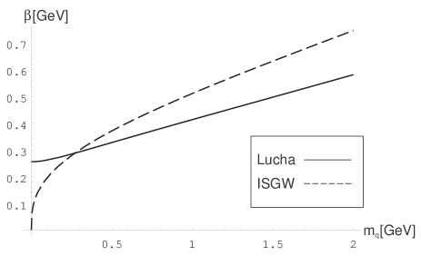
Figure 2: ISGW[20] and Lucha[23] model $\beta$’s for pseudoscalar $|q\bar{q}\rangle$

In the relativistic approach one finds sizable $\beta$ values (comparable with nonrealtivistic ones), for small quark masses also. For $q\bar{q}$ pairs the ratios among calculated masses are for example $m_{NR}(u\bar{d})/m_{R}(u\bar{d})\cong 0.7$, $m_{NR}(u\bar{s})/m_{R}(u\bar{s})\cong 0.8$.

The scalar meson masses can be connected with (A7) by

$$M_{0}=\frac{\sum_{f}C_{f}^{2}(f(\beta,m_{q})+h(\beta,m_{q}))}{\sum_{f}C_{f}^{2}\ g(\beta,m_{q})}$$ (A8)

$$f(\beta,m_{q})=\int_{0}^{\infty}4\pi p^{2}\,dp\frac{2p^{2}\phi_{f}^{2}}{p^{2}+m_{f}^{2}}2\epsilon_{f}$$ (A9)

$$h(\beta,m_{q})=\int_{0}^{\infty}4\pi p^{2}\,dp\frac{2p^{2}\phi_{f}^{2}}{p^{2}+m_{f}^{2}}V(p)$$ (A10)

$$g(\beta,m_{q})=\int_{0}^{\infty}4\pi p^{2}\,dp\frac{2p^{2}\phi_{f}^{2}}{p^{2}+m_{f}^{2}}$$ (A11)

This is just the expression (A.4) in meson rest frame with (A7) included and $g$ is normalization. With the potential (A7)$(c=0,\alpha=0.63)$ one finds for example for $a_{0}(980):\beta=0.284$ and $M_{0}=977\ MeV$. It is useful to note that one obtains $h=0$ for $\beta=0.288$ and $\sum h/g\cong 0.011\ MeV$ for $\beta=0.284$. Thus the expressions (A.4) and (A.8) are numerically consistent for our range of parameters.

The model also satisfies a very general condition (2.9). Using

$$V^{\mu}(0)=\sum_{f}:\overline{\Psi}_{f}(0)\gamma^{\mu}\Psi_{f}(0):$$ (A12)

where

$$\Psi_{f}(0)=\sum_{s}\int\frac{d^{3}l}{(2\pi)^{3}}\frac{m_{f}}{E_{f}}[b_{f}(\vec{l},s)u_{f}(\vec{l},s)+d^{+}_{f}(\vec{l},s)v_{f}(\vec{l},s)]$$ (A13)

the condition (2.12) can be explicitly written as:

$$\langle 0|V^{\mu}(0)|f_{0}\rangle=\frac{1}{(2\pi)^{3/2}}I(\vec{p},\vec{q})\frac{m_{1}q^{\mu}-m_{2}p^{\mu}}{m_{1}m_{2}}$$ (A14)

The conserved vector current requires equal quark masses, i.e $m_{1}=m_{2}$. In the rest frame $E=M,\ \vec{P}=0$, $\vec{p}=-\vec{q}$, $\epsilon=e$. For the time component of (A6) one obtains

$$\frac{m_{1}q^{0}-m_{2}p^{0}}{m_{1}m_{2}}=\frac{\epsilon-e}{m_{1}}=0.$$ (A15)

The spatial components $\mu=1,2,3$ vanish after the integration over $d^{3}p$ in $I(\vec{p},\vec{q})$ (3.7).

A more general scalar meson state than (2.1) can be constructed by replacing

$$\overline{u}_{f}v_{f}\rightarrow\overline{u}_{f}(a+b\frac{\not\!P}{M})v_{f}$$ (A16)

and by adjusting the normalization accordingly. It can be shown that the term proportional to $b$ neither influences the normalization, nor contributes to the decay width (3.15) within conventions, such as for example (2.4), which were used here. Therefore the simpler form (2.1) was used.

References

• [1] R. M. Barnett et al., Phys. Rev. D 54, 1 (1996).
• [2] D. Morgan and M. R. Pennington, Phys. Rev. D 48, 5422 (1993).
• [3] B. S. Zou and D. V. Bug, Phys. Rev. D 48, 3948 (1993).
• [4] G. Jansen et al., Phys. Rev. D 52, 2690 (1995).
• [5] J. Wienstein and N. Isgur, Phys. Rev. D 41, 2236 (1990).
• [6] F. E. Close et al., Phys. Lett. B 319, 291 (1993).
• [7] N. A. TΓΆrnquist, Z. Phys. C 68, 647 (1995).
• [8] A. Bramon and S. Narison, Mod. Phys. Lett. A 4, 1113 (1989).
• [9] M. Genovese, Nuovo Cim. A 107, 1249 (1994).
• [10] A. S. Deakin et al., Mod. Phys. Lett. A 9, 2381 (1994).
• [11] J. Babckock and J. L. Rosner, Phys. Rev. D 14, 1286 (1976).
• [12] A. Bramon, Phys. Lett. B 333, 153 (1994).
• [13] J. Lanik, Phys. Lett. B 306, 139( 1993).
• [14] S. Fajfer, Z. Phys. C 68, 81 (1995).
• [15] N. N. Achasov et al., Phys. Lett. B 108, 134 (1982).
• [16] N. N. Achasov, hep-ph/9803292;
M. N. Achasov et al., Phys. Lett. B 481, 441 (1998).
• [17] M. Boglione and M. R. Pennington, hep-ph/9812258.
• [18] D. TadiΔ‡ and S. Ε½ganec, Phys. Rev. D 52, 6466 (1995).
• [19] D. TadiΔ‡ and S. Ε½ganec, in Hadron 1995, eds. M.C. Birse, G.D. Laferty and J.A.McGovern (World Scientific, Singapore, 1996).
• [20] N. Isgur, D. Scora, B. Grinstein, and M.B. Wise, Phys. Rev. D 39, 799 (1989);
D. Scora and N. Isgur, Phys. Rev. D 52, 2783 (1995).
• [21] N. Brambilla and A. Vairo, Phys. Rev. D 55, 3974 (1997).
• [22] G. S. Bali, K. Schilling and A. Wachter, Phys. Rev. D 56, 2566 (1997).
• [23] W. Lucha, H. Rupprecht and F.F. SchΓΆberl, Phys. Rev. D 44, 242 (1991).