Abstract

Data from HERA, LEP and the Tevatron, as well as from low energy experiments are used to constrain the scale of possible electron-quark contact interactions. Different models are considered, including the most general one, in which all new couplings can vary independently. Limits on couplings and mass scales are extracted and upper limits on possible effects to be observed in future HERA, LEP and Tevatron running are estimated. Total hadronic cross-section at LEP and $e^{-}p$ scattering cross-section at HERA are strongly constrained by existing data, whereas large cross-section deviations are still possible for Drell-Yan lepton pair production at the Tevatron.

1 Introduction

Search for ”new physics” has always been one of the most exciting subjects in the field of particle physics. The results presented in 1997 by the H1 [1] and ZEUS [2] experiments at HERA electrified the physics community. Both experiments reported an excess of events in positron-proton Neutral Current Deep Inelastic Scattering (NC DIS) at very high momentum transfer scales $Q^{2}$, as compared with the predictions of the Standard Model. Unfortunately, in spite of the significant increase in the integrated data luminosity, these results have not been confirmed nor contradicted[3, 4]. The effect can be just due to a statistical fluctuation, but can also be a first sign of some ”new physics”.

In 1998 HERA experiments started again to collect electron-proton data aiming for integrated luminosity comparable with that of the positron-proton data. The first results are expected soon. The aim of the presented analysis is to review experimental and theoretical constraints on possible signals of ”new physics” at HERA and extract limits on a new effects to be seen in the new HERA $e^{-}p$ data. Limits corresponding to other present and future high-energy experiments are also considered. The contact interaction models, used as the general framework for this analysis are described in section 2. In section 3 the relevant data from HERA, LEP, the Tevatron and other experiments are briefly described. Methods used to compare data with contact interaction model predictions are discussed in section 4. The results of analysis within different contact interaction models, including extracted limits on the mass scale of new interactions, are presented in section 5. Predictions for the future discovery potential at HERA, as well as at LEP and the Tevatron are discussed in section 6.

The analysis presented here is based on the approach suggested in [5]. Significant work has been done to improve the treatment of experimental data, including a proper interpretation of statistical and systematic errors as well as acceptance cuts and smearing.

2 Contact Interactions

Four-fermion contact interactions are an effective theory, which allows us to describe, in the most general way, possible low energy effects coming from ”new physics” at much higher energy scales. This includes the possible existence of second generation heavy weak bosons, leptoquarks as well as electron and quark compositeness [6, 7]. Contact interactions can be represented as additional terms in the Standard Model Lagrangian [7]:

$$L_{CI} = \eta_{s}(\bar{e}_{L}e_{R})(\bar{q}_{L}q_{R})+\eta_{s}^{\prime}(\bar{e}_{L}e_{R})(\bar{q}_{R}q_{L})+h.c.\hskip 71.13188pt\rm scalar$$

$$+ \sum_{i,j=L,R}\eta_{ij}(\bar{e}_{i}\gamma^{\mu}e_{i})(\bar{q}_{j}\gamma_{\mu}q_{j})\hskip 145.10922pt\rm vector$$

$$+ \eta_{T}(\bar{e}_{L}\sigma^{\mu\nu}e_{R})(\bar{q}_{L}\sigma_{\mu\nu}q_{R})+h.c.\hskip 125.19194pt\rm tensor$$

where subsequent lines describe the scalar, vector and tensor contact interaction terms respectively. As very strong limits have been already placed on both scalar and tensor terms [7] this paper considers vector terms only.

The influence of the vector contact interactions on the $ep$ NC DIS cross-section can be described as an additional term in the tree level $eq\rightarrow eq$ scattering amplitude [5]:

$$M^{e_{i}q_{j}\rightarrow e_{i}q_{j}}(t) = -\frac{4\pi\alpha_{em}e_{q}}{t}\;+\;\frac{4\pi\alpha_{em}}{sin^{2}\theta_{W}\cdot cos^{2}\theta_{W}}\cdot\frac{g^{e}_{i}g^{q}_{j}}{t-M_{Z}^{2}}\;+\;\eta^{eq}_{ij}$$ (2)

where $t=-Q^{2}$ is the Mandelstam variable describing the four-momentum transfer between the electron and the quark, $e_{q}$ is the electric charge of the quark in units of the elementary charge and the subscripts $i$ and $j$ label the chiralities of the initial lepton and quark respectively: $i,j=L,R$. $g^{e}_{i}$ and $g^{q}_{j}$ are electroweak couplings of the electron and the quark

$$g^{f}_{L} = I_{3f}-e_{f}\sin^{2}\theta_{W}$$ (3)

$$g^{f}_{R} = \;\;\;\;\;-e_{f}\sin^{2}\theta_{W}$$

where $I_{3f}$ is the third component of the SU(2) isospin for the fermion $f$: $f=e,q$.

For processes such as $e^{+}e^{-}\rightarrow hadrons$ or $p\bar{p}\rightarrow l^{+}l^{-}X$, a corresponding formula can be written for the $e^{+}e^{-}\rightarrow q\bar{q}$ tree level amplitude:

$$M^{e_{i}\bar{e}_{j}\rightarrow q_{i}\bar{q}_{j}}(s) = -\frac{4\pi\alpha_{em}e_{q}}{s}\;+\;\frac{4\pi\alpha_{em}}{sin^{2}\theta_{W}\cdot cos^{2}\theta_{W}}\cdot\frac{g^{e}_{i}g^{q}_{j}}{s-M_{Z}^{2}+is\frac{\Gamma_{Z}}{M_{Z}}}\;+\;\eta^{eq}_{ij}$$ (4)

where $s$ is the center-of-mass energy squared of the four-fermion reaction. The sign of the contact interaction contribution to the $s$-channel amplitude (4) is the same as for the $t$-channel amplitude (2). However, the Standard Model amplitude changes its sign due to the opposite signs of $s$ and $t$ variables. It is therefore important to notice that the resulting sign of the interference terms in the cross-section for $e^{\pm}p$ scattering is different from that in $e^{+}e^{-}$ or $p\bar{p}$ scattering.

The contact interaction coupling strength $\eta$ can be related to the mass scale ${\cal M}$ of new physics through the formula:

$$\eta = \pm\frac{g_{CI}^{2}}{{\cal M}^{2}}$$

where $g_{CI}$ is the unknown coupling strength of new interactions. As the contact interaction contribution always depends on the $g_{CI}$ to ${\cal M}$ ratio, it is convenient to consider the effective mass scale $\Lambda$ defined through the formula:

$$\eta = \pm\frac{4\pi}{\Lambda^{2}}$$

which corresponds to the choice $g^{2}_{CI}=4\pi$.

2.1 General Model

In the most general case, vector contact interactions are described by 4 independent couplings for every lepton-quark pair. With only 2 lepton ($e$ and $\mu$) and 5 quark flavours (i.e. neglecting $t$ quark contribution), we still have 40 independent couplings. It would be very difficult, if not impossible, to consider the model with 40 free parameters. However, some of these parameters (couplings) are weakly constrained by existing experimental data. To reduce the number of the free model parameters, weakly constrained couplings can be either neglected or additionally constrained by relating them to some other couplings.

Most of existing experimental data is sensitive predominantly to electron-up and electron-down quark couplings. Therefore, the first model considered in this analysis is the one assuming that these 8 couplings ($\eta^{ed}_{LL}$, $\eta^{ed}_{LR}$, $\eta^{ed}_{RL}$, $\eta^{ed}_{RR}$, $\eta^{eu}_{LL}$, $\eta^{eu}_{LR}$, $\eta^{eu}_{RL}$, $\eta^{eu}_{RR}$) can vary independently, whereas other couplings (for $s$, $c$, $b$, $t$ quarks and/or $\mu$, $\tau$ leptons) are assumed to vanish. This case will be referred to as the general model.

The other possibility is to impose additional relations between couplings. The common choice is to assume lepton universality:

$$\eta^{eq}_{ij} =\eta^{\mu q}_{ij} =\eta^{\tau q}_{ij}$$ (5)

and quark family universality:

$$\eta^{eu}_{ij} =\eta^{ec}_{ij} =\eta^{et}_{ij}$$ (6)

$$\eta^{ed}_{ij} =\eta^{es}_{ij} =\eta^{eb}_{ij}$$

Lepton universality allows us to include data on muon pair production at the Tevatron (see section 3.2), whereas assuming quark family universality significantly improves the constraints which we can obtain from LEP2 measurements (see section 3.3). As a result, experimental constraints on contact interactions can be significantly improved without increasing the number of free model parameters. The model assuming relations (5) and (6) will be referred to as the model with family universality.

2.2 $SU(2)_{L}\times U(1)_{Y}$ Universality

Another commonly used assumption about lepton-quark contact interactions is that they satisfy the $SU(2)_{L}\times U(1)_{Y}$ gauge invariance of the Standard Model. Assuming that left-handed electrons and quarks belong to $SU(2)_{L}$ doublets and that the contact interaction Lagrangian (2) respects the $SU(2)_{L}$ symmetry implies a relation between contact terms involving left-handed $u$ and $d$ quarks [5]:

$$\eta^{eu}_{RL} = \eta^{ed}_{RL}$$

which reduces the number of free model parameters from 8 to 7. The $SU(2)_{L}\times U(1)_{Y}$ also relates $eeqq$ contact interaction couplings with those of $\nu\nu qq$ interactions

$$\eta^{\nu u}_{LL} = \eta^{ed}_{LL}$$ (7)

$$\eta^{\nu d}_{LL} = \eta^{eu}_{LL}$$

$$\eta^{\nu u}_{LR} = \eta^{eu}_{LR}$$

$$\eta^{\nu d}_{LR} = \eta^{ed}_{LR}$$

This allows us to use, in the study of $eeqq$ contact interactions, additional data on NC neutrino scattering (see section 3.4).

Moreover, assuming the $SU(2)_{L}\times U(1)_{Y}$ universality introduces a related contact interaction term in the Charged Current process $eq\rightarrow\nu q^{\prime}$. The coupling constant for the induced Charged Current contact interaction is

$$\eta^{CC}\equiv\eta^{eu\nu d} = \eta^{ed}_{LL}-\eta^{eu}_{LL}$$ (8)

This relation allows us to use, in the study of Neutral Current contact interaction, also data from Charged Current processes (see section 3.1 and 3.4).

The model assuming the $SU(2)_{L}\times U(1)_{Y}$ universality will be referred to as the SU(2) model. In order to reduce the number of models, the SU(2) models considered in this analysis always assume lepton and quark family universality.

2.3 One-parameter models

Using data from a single experiment it is mostly not possible to put significant constraints on contact interaction scales in the general case. Therefore it is a common practise to consider particular models, which assume fixed relations between the separate couplings, reducing the number of free parameters to one. For example, the so called vector-vector model assumes that all couplings are equal:

$$\eta^{ed}_{LL}=\eta^{ed}_{LR}=\eta^{ed}_{RL}=\eta^{ed}_{RR}=\eta^{eu}_{LL}=\eta^{eu}_{LR}=\eta^{eu}_{RL}=\eta^{eu}_{RR} \equiv \eta_{VV}$$

Mass scale limits obtained in one-parameter models are, artificially, much stronger than in the general model. They will be considered in this analysis to allow comparison with other results. The relations between couplings assumed for different models are listed in Table 1[11]. It should be noticed that all one-parameter models considered assume

$$\eta^{eq}_{LL}+\eta^{eq}_{LR}-\eta^{eq}_{RL}-\eta^{eq}_{RR} = 0$$

for $q=u,d$, to avoid strong limits coming from atomic parity violation measurements (see section 3.4). For all one-parameter models quark and lepton family universality is assumed. The results obtained both with and without imposing the $SU(2)_{L}\times U(1)_{Y}$ universality are presented, except for the U2, U4 and U6 models, which violate it explicitly ($\eta^{eu}_{RL}\neq\eta^{ed}_{RL}$).

Model	$\eta^{ed}_{LL}$	$\eta^{ed}_{LR}$	$\eta^{ed}_{RL}$	$\eta^{ed}_{RR}$	$\eta^{eu}_{LL}$	$\eta^{eu}_{LR}$	$\eta^{eu}_{RL}$	$\eta^{eu}_{RR}$
VV	$+\eta$	$+\eta$	$+\eta$	$+\eta$	$+\eta$	$+\eta$	$+\eta$	$+\eta$
AA	$+\eta$	$-\eta$	$-\eta$	$+\eta$	$+\eta$	$-\eta$	$-\eta$	$+\eta$
VA	$+\eta$	$-\eta$	$+\eta$	$-\eta$	$+\eta$	$-\eta$	$+\eta$	$-\eta$
X1	$+\eta$	$-\eta$			$+\eta$	$-\eta$
X2	$+\eta$		$+\eta$		$+\eta$		$+\eta$
X3	$+\eta$			$+\eta$	$+\eta$			$+\eta$
X4		$+\eta$	$+\eta$			$+\eta$	$+\eta$
X5		$+\eta$		$+\eta$		$+\eta$		$+\eta$
X6			$+\eta$	$-\eta$			$+\eta$	$-\eta$
U1					$+\eta$	$-\eta$
U2					$+\eta$		$+\eta$
U3					$+\eta$			$+\eta$
U4						$+\eta$	$+\eta$
U5						$+\eta$		$+\eta$
U6							$+\eta$	$-\eta$

Table 1: Relations between couplings for the one-parameter models considered in this paper.

3 Experimental Data

In this section the data used to constrain contact interaction model are presented. For each measurement, the formula describing the possible influence of the new couplings on the measured quantities is given. Description of the statistical methods used to interpret the data will be presented in the section 4.

3.1 High-$Q^{2}$ DIS at HERA

Used in this analysis are the latest data on high-$Q^{2}$ $e^{+}p$ NC DIS from both H1 [3] and ZEUS [4], corresponding to integrated data luminosities of 37 and 47$pb^{-1}$, respectively. Older results from $e^{-}p$ NC DIS scattering [8, 9] are also used, although the influence of these data is marginal. For models with the $SU(2)_{L}\times U(1)_{Y}$ universality, as mentioned in section 2, data on $e^{+}p$ CC DIS [3, 10] are also included in the fit.

HERA experiments quote their high-$Q^{2}$ DIS results in terms of numbers of events and/or cross-sections measured in bins of $Q^{2}$. For simplicity let us consider a single $Q^{2}$ bin ranging from $Q^{2}_{min}$ to $Q^{2}_{max}$. Assume that $n_{SM}$ events are expected from the Standard Model.

The leading order doubly-differential cross-section for positron-proton NC DIS ($e^{+}p\rightarrow e^{+}X$) can be written as [5]

$$\frac{d^{2}\sigma^{LO}}{dxdQ^{2}} = \frac{1}{16\pi}\sum_{q}q(x)\left\{|M^{eq}_{LR}|^{2}+|M^{eq}_{RL}|^{2}+(1-y)^{2}\left[|M^{eq}_{LL}|^{2}+|M^{eq}_{RR}|^{2}\right]\right\}\;+$$

$$~{}~{}~{}~{}~{}~{}~{}~{}~{}~{}\bar{q}(x)\left\{|M^{eq}_{LL}|^{2}+|M^{eq}_{RR}|^{2}+(1-y)^{2}\left[|M^{eq}_{LR}|^{2}+|M^{eq}_{RL}|^{2}\right]\right\}$$

where $x$ is the Bjorken variable, describing the fraction of proton momentum carried by a quark (antiquark), $q(x)$ and $\bar{q}(x)$ are the quark and antiquark momentum distribution functions in the proton and $M^{eq}_{ij}$ are the scattering amplitudes of equation (2), which can include contributions from contact interactions described by a set of couplings $\vec{\eta}$.

The cross-section (including the contribution from contact interactions), integrated over the $x$ and $Q^{2}$ range of an experimental $Q^{2}$ bin is

$$\sigma^{LO}(\vec{\eta}) = \displaystyle\int\limits_{Q^{2}_{min}}^{Q^{2}_{max}}dQ^{2}\displaystyle\int\limits_{\frac{Q^{2}}{s\cdot y_{max}}}^{1}dx\;\frac{d^{2}\sigma^{LO}(\vec{\eta})}{dxdQ^{2}}$$ (9)

where $y_{max}$ is the upper limit on reconstructed Bjorken variable $y$ imposed in the analysis. The number of events expected from the Standard Model with contact interaction contributions can now be calculated as:

$$n(\vec{\eta}) = n_{SM}\cdot\left(\frac{\sigma^{LO}(\vec{\eta})}{\sigma^{LO}_{SM}}\right)$$ (10)

where $\sigma^{LO}_{SM}$ is the Standard Model cross-section calculated with formula (9) (setting $\vec{\eta}=\vec{0}$). Leading-order expectations of the contact interaction models are used to rescale the Standard Model prediction $n_{SM}$ coming from detailed experiment simulation. This accounts not only for different experimental effects, but also for higher order QCD and electroweak corrections. Validity of this approach is discussed in section 4.

3.2 Drell-Yan lepton pair production at the Tevatron

Used in this analysis are data on Drell-Yan lepton pair production from the CDF [12] and D0 [13] experiments. Both experiments present numbers of measured high-mass electron pairs ($p\bar{p}\rightarrow e^{+}e^{-}\;X$). CDF also presents results on muon pair production ($p\bar{p}\rightarrow\mu^{+}\mu^{-}\;X$), which are used in the case of models with family universality (see section 2).

The leading order cross-section for lepton pair production in $p\bar{p}$ collisions is

$$\frac{d^{2}\sigma^{LO}}{dM_{ll}dY} = \frac{M_{ll}^{3}}{72\pi s}\sum_{q}q(x_{1})q(x_{2})\sum_{i,j=L,R}|M^{eq}_{ij}|^{2}$$

where $M_{ll}$ is the invariant mass of lepton pair, $Y$ is the rapidity of the lepton pair center-of-mass frame, $x_{1}$ and $x_{2}$ are the fractions of proton and antiproton momenta carried by the annihilating quarks. The scattering amplitudes $M^{eq}_{ij}$ and the parton density functions are calculated for scale

$$\hat{s} = x_{1}x_{2}s$$

where $s$ is the total proton-antiproton center of mass energy squared.

The cross-section corresponding to the $M_{ll}$ range from $M_{min}$ to $M_{max}$ is calculated as

$$\sigma^{LO}(\vec{\eta}) = \displaystyle\int\limits_{M_{min}}^{M_{max}}dM_{ll}\displaystyle\int\limits_{-Y_{max}}^{Y_{max}}dY\;A_{ll}(Y)\cdot\frac{d^{2}\sigma(\vec{\eta})}{dM_{ll}dY}$$ (11)

where $Y_{max}$ is the upper limit on the rapidity of the produced lepton pair:

$$Y_{max} = \ln\frac{\sqrt{s}}{M_{ll}}\;,$$

and $A_{ll}(Y)$ is the acceptance function, resulting from the integration over the lepton pair production angle in the center of mass system, with angular detector coverage taken into account. The cross-section calculated with equation (11) is used to calculate the number of events expected from the Standard Model with contact interaction contributions using formula (10).

3.3 Measurements from LEP

Many measurements at LEP are sensitive to different kinds of ”new physics”. The $eeqq$ contact interactions can be directly tested in the measurement of the total cross-section for $e^{+}e^{-}\rightarrow q\bar{q}$. Using flavour tagging techniques, additional constraints can be obtained from the measurement of the heavy quark decay fractions $R_{b}$ and $R_{c}$, and of the forward-backward asymmetries $A^{q}_{FB}$ of $q\bar{q}$ events.

The leading order formula for the total quark pair production cross-section $e^{+}e^{-}\rightarrow q\bar{q}$, at the total electron-positron center of mass energy squared $s$, is

$$\sigma^{LO}(s) = \frac{s}{16\pi}\sum_{q}\sum_{i,j=L,R}|M^{eq}_{ij}|^{2}$$ (12)

where $M^{eq}_{ij}$ are the scattering amplitudes described by equation (4), including contributions from contact interaction couplings $\vec{\eta}$. For comparison with measured experimental values, the leading order contact interaction cross-sections are rescaled using the expected Standard Model cross-section $\sigma^{SM}(s)$ quoted by experiments:

$$\sigma(s,\vec{\eta}) = \sigma^{SM}(s)\cdot\left(\frac{\sigma^{LO}(s,\vec{\eta})}{\sigma^{LO}(s,0)}\right)$$ (13)

where $\sigma^{LO}(s,0)$ is the leading-order Standard Model cross-section ($\vec{\eta}=\vec{0}$), calculated with equation (12). This takes into account possible experimental effects and higher order QCD and electroweak corrections (for discussion see section 4). All four LEP experiments have recently presented data on $\sigma_{had}$ for center-of-mass energies up to 189 GeV [14, 15, 16, 17, 18].

The sensitivity of the total hadronic cross-section to the contact interaction coupling strength $\vec{\eta}$ is limited by the fact that the interference terms in the quark-pair production cross-sections have opposite signs for up-type and down-type quarks. In the total cross-section, summed over all quark flavours, these terms tend to compensate each other. However, if this is the case, the fraction of events produced with the given quark-pair flavour turns out to be very sensitive to the contact interaction couplings.

Using different flavour tagging techniques, cross-sections for $b\bar{b}$ and $c\bar{c}$ pair production and the corresponding fractions $R_{b}$ and $R_{c}$ can be measured. Although the limited tagging efficiency and purity significantly affects the measurement, useful constraints on contact interaction couplings can be extracted. Used in this analysis are results on $R_{b}$ coming from Aleph[14, 19], Delphi [15] and Opal [20] as well as Delphi results on $R_{c}$ [15].

The contact interaction contribution to the scattering amplitude affects also the observed forward-backward asymmetry of $q\bar{q}$ events. In the leading order the forward-backward asymmetry can be calculated as

$$A^{q}_{FB}(s) = \frac{3}{4}\cdot\frac{|M^{eq}_{LL}|^{2}-|M^{eq}_{LR}|^{2}-|M^{eq}_{RL}|^{2}+|M^{eq}_{RR}|^{2}}{|M^{eq}_{LL}|^{2}+|M^{eq}_{LR}|^{2}+|M^{eq}_{RL}|^{2}+|M^{eq}_{RR}|^{2}}$$

where the factor $\frac{3}{4}$ corresponds to the integration over the full angular range.

Constraints upon the forward-backward asymmetries $A^{q}_{FB}$ are obtained using a jet charge technique. After clustering all the events into two jets, the jet charge $Q_{jet}$ of each jet can be determined from the momentum weighted sum over all charged tracks in the jet. The sign of $Q_{jet}$ coincides with the charge of produced quark in about 70% of events. The forward-backward asymmetry for the selected sample of events (e.g. $b$-tagged events) can be extracted in two ways. The method used by Aleph is based on the measurement of the mean charge difference between the forward and backward jets $\langle Q_{FB}\rangle=\langle Q^{F}_{jet}\rangle-\langle Q^{B}_{jet}\rangle$. Delphi and Opal extract $A^{q}_{FB}$ from the angular distribution of jets with well defined sign. In both cases, the measured asymmetry depends on the parton-level asymmetries $A^{q}_{FB}$ and on the quark content of the selected sample. As the up-type and down-type quarks have charges of opposite signs, the measured asymmetry is very sensitive to the relative contribution of different quark flavours. Even if we measure the asymmetry for the flavour-tagged sample, the selected sample of events is always contaminated by other quark flavours (e.g. a $b$-tagged sample always contains a fraction of $c\bar{c}$ events) and the measured value depends strongly on the quark production fractions (e.g. $R_{b}$ and $R_{c}$). This is the reason why the measurement of the forward-backward asymmetry is very sensitive to the contact interaction couplings. Used in this analysis are the measurements of forward-backward asymmetry for the $b$-tagged events [14, 15, 20], $c$-tagged events [15] and anti-tagged events [14, 15].

3.4 Data from low energy experiments

The low energy data are included in the present analysis in the manner which follows closely the approach presented in [5, 21]. Therefore only basic assumptions are listed here and technical details are omitted.

In case of the general contact interaction model the following constraints from low energy experiments are considered:

• Atomic Parity Violation (APV)
  The Standard Model predicts parity non-conservation in atoms caused (in lowest order) by the $Z^{\circ}$ exchange between electrons and quarks in the nucleus. Experimental results on parity violation in atoms are given in terms of the weak charge $Q_{W}$ of the nuclei. A very precise determination of $Q_{W}$ for Cesium atoms was recently reported [22]. The experimental result differs from the Standard Model prediction [23, 24] by:

  $$\Delta Q_{W}^{Cs}\equiv Q_{W}^{meas}-Q_{W}^{SM} = 0.71\pm 0.84$$

  Corresponding results have also been obtained for thallium [25, 24]:

  $$\Delta Q_{W}^{Tl} = 1.9\pm 3.6\;.$$

  These measurements are used to place limits on contact interaction contributions to $Q_{W}$:

  $$\Delta Q_{W}(\vec{\eta}) = \frac{2Z+N}{\sqrt{2}G_{F}}\left(\eta^{eu}_{LL}+\eta^{eu}_{LR}-\eta^{eu}_{RL}-\eta^{eu}_{RR}\right)$$

  $$+ \frac{Z+2N}{\sqrt{2}G_{F}}\left(\eta^{ed}_{LL}+\eta^{ed}_{LR}-\eta^{ed}_{RL}-\eta^{ed}_{RR}\right)$$

• electron-nucleus scattering
  The limits on possible contact interaction contributions to electron-nucleus scattering at low energies can be extracted from the polarisation asymmetry measurement

  $$A = \frac{d\sigma_{R}-d\sigma_{L}}{d\sigma_{R}+d\sigma_{L}}$$

  where $d\sigma_{L(R)}$ denotes the differential cross-section of left- (right-) handed electron scattering. Polarisation asymmetry directly measures the parity violation resulting from the interference between the weak ($Z^{\circ}$ exchange) and the electro-magnetic ($\gamma$ exchange) scattering amplitudes. For isoscalar targets, taking into account valence quark contributions only, the polarisation asymmetry for elastic electron scattering is

  $$A_{el} = -\frac{3\sqrt{2}G_{F}Q^{2}}{20\pi\alpha_{em}}\left[2\left(g^{u}_{L}+g^{u}_{R}\right)-\left(g^{d}_{L}+g^{d}_{R}\right)\right]$$

  where $Q^{2}$ is the four-momentum transfer and $g^{q}_{i}$ are quark electroweak couplings, as introduced in equation (3). Contact interactions modify the effective quark electroweak coupling

  $$\left.{g^{q}_{i}}\right|_{ef\!f} = g^{q}_{i}-\frac{\eta^{eq}_{Li}}{2\sqrt{2}G_{F}}$$ (14)

  The constraints used in this analysis come from the SLAC $e$D experiment [26], the Bates $e$C experiment [27] and the Mainz experiment on $e$Be scattering [28]. In case of models with family universality also data from the $\mu^{\pm}$C experiment at CERN[29] are included.

In case of the SU(2) models additional constraints come from:

• neutrino-nucleus scattering
  Constraints on the couplings of quarks to the $Z^{\circ}$ and/ or additional $\nu\nu qq$ contact interactions (related to $eeqq$ CI, as described in section 2.2) can also be derived from the precise measurement of the ratio of Neutral Current to Charged Current neutrino-nucleon scattering cross sections

  $$R^{\nu} = \frac{\sigma^{\nu N}_{{}_{NC}}}{\sigma^{\nu N}_{{}_{CC}}}\;.$$

  However, when using constraints on $g^{q}_{i}$ resulting from measurement of $R^{\nu}$, one also has to take into account that possible contact interaction contribution affects not only the Neutral Current but also the Charged Current scattering cross-section (see section 2.2). Therefore the quark electroweak coupling extracted from $R^{\nu}$ measurements should be expressed as

  $$\left.{g^{q}_{i}}\right|_{meas} = \frac{g^{q}_{i}-\frac{\eta^{\nu q}_{Li}}{2\sqrt{2}G_{F}}}{1-\frac{\eta^{CC}}{4\sqrt{2}G_{F}}}$$

  It is important to notice that $\eta^{eq}_{Li}$ entering formula (14) has been replaced here by $\eta^{\nu q}_{Li}$. This is because the effective $g^{u}_{L}$ and $g^{d}_{L}$ couplings measured in neutrino scattering are sensitive to “flavour crossed” contact interaction couplings $\eta^{ed}_{LL}$ and $\eta^{eu}_{LL}$ respectively, which results from relations (7). Experimental constraints on $R^{\nu}$ come mainly from muon-neutrino experiments. Assuming lepton and quark family universality, the following measurements of $g^{q}_{i}$ from $\nu_{\mu}N$ scattering are used: the results compiled by Fogi and Haidt [30] and the recent constraints from CCFR[31] and NuTeV[32].

• lepton-hadron universality of weak Charged Currents
  Charged Current contact interactions which are induced by $SU(2)_{L}\times U(1)_{Y}$ universality (see equation (8)) would also affect the measurement of $V_{ud}$ element of the Cabibbo-Kobayashi-Maskawa (CKM) matrix, leading to the effective violation of unitarity [33, 34]. The current experimental constraint is [24]

  $$|V_{ud}|^{2}+|V_{us}|^{2}+|V_{ub}|^{2} = 0.9969\pm 0.0022$$

  whereas the expected contribution from the contact interaction is

  $$\left.{V_{ud}}\right|_{meas} = V_{ud}^{SM}\cdot\left(1-\frac{\eta^{CC}}{4\sqrt{2}G_{F}}\right)$$

• electron-muon universality
  In the similar way Charged Current contact interactions would also lead to effective violation of $e$-$\mu$ universality in charged pion decay [33]. The current experimental value of $R=\Gamma(\pi^{-}\rightarrow e\bar{\nu})/\Gamma(\pi^{-}\rightarrow\mu\bar{\nu})$ is [35]

  $$\frac{R_{meas}}{R_{SM}} = 0.9966\pm 0.030$$

  whereas the expected contribution from the contact interaction is

  $$\left.{R}\right|_{meas} = R_{SM}\cdot\left(1-\frac{\eta^{CC}}{4\sqrt{2}G_{F}}\right)^{2}$$

It is interesting to notice, that data in Charged Current sector may point to a slight violations of the unitarity of the CKM matrix and of the $e$-$\mu$ universality. Both measurements are consistent with the presence of CC contact interactions with a mass scale of the order of 10 TeV. The combined significance of these two results is about 1.8$\sigma$, but it has a considerable influence on global analysis results for the SU(2) model.

4 Analysis method

The aim of this study is to find the allowed ranges for contact interaction couplings within the different models considered. To do so, the probability function in the coupling space,

$${\cal P}(\vec{\eta}) \sim \prod_{i}P_{i}(\vec{\eta}),$$ (15)

is calculated. In (15), the product runs over all experimental data $i$ and $\vec{\eta}$ represents the set of free parameters for a given model (one or many). This section describes how the probability function is defined and which corrections are included to take into account experimental conditions.

4.1 Statistical errors

All experimental data used in this analysis can be divided into two classes.

1. For experiments in which a result can be presented as a single number with an error which is considered to reflect a Gaussian probability distribution, the constraints on the contact interaction couplings can be usually expressed using the equation

   $$F(\vec{\eta}) = \Delta A\;\pm\;\sigma_{A}$$

   where $\Delta A$ is the difference between the measured value and the Standard Model prediction, and $F(\vec{\eta})$ is the expected contact interaction contribution to the measured value of A. The resulting probability function can be written as

   $$P_{i}(\vec{\eta}) \sim exp\left(-\frac{1}{2}\frac{(F(\vec{\eta})-\Delta A)^{2}}{\sigma_{A}^{2}}\right)$$ (16)

   reflecting the definition of the Gaussian error $\sigma_{A}$. This approach is used for all low energy data as well as for the LEP hadronic cross-section measurements.

2. On the other hand, when the experimentally measured quantity is the number of events of a particular kind (e.g. HERA high-$Q^{2}$ events or Drell-Yan lepton pairs at the Tevatron), and especially when this number is small, the probability is better described by the Poisson distribution

   $$P_{i}(\vec{\eta}) \sim \frac{n(\vec{\eta})^{N}\cdot exp(-n(\vec{\eta}))}{N!}$$ (17)

   where $N$ and $n(\vec{\eta})$ are the measured and expected number of events in a given experiment, respectively, and $n(\vec{\eta})$ takes into account a possible contact interaction contribution. This approach has been used for HERA and the Tevatron data.

4.2 Systematic errors

For low energy data the total measurement error can be used in formula (16) taking into account both statistical and systematic errors. For collider data, formula (16) or (17) is used to take into account the statistical error of the measurement only. As for the systematic errors, it is assumed that within a given data set (e.g. $e^{+}p$ NC DIS data from ZEUS ) they are correlated to 100%. This seems to be a much better approximation of the experimental conditions than assuming that systematic errors are uncorrelated. In fact most of the contributing systematic uncertainties at HERA are highly correlated between different $Q^{2}$ bins, as for example energy scale uncertainty or the luminosity measurement.

For each data set, a common systematic shift parameter $\delta$ has been introduced to describe the possible variation of event numbers expected at HERA or the Tevatron, or cross-sections predicted at LEP, due to systematic error:

$$n_{SM} = \bar{n}_{SM}\;+\;\delta\cdot\sigma_{n}^{sys}$$

$${\rm or}\;\;\;\;\;\;\;\;\;\sigma^{SM} = \bar{\sigma}_{SM}\;+\;\delta\cdot\sigma_{\sigma}^{sys}$$

where $\bar{n}_{SM}$ ($\bar{\sigma}_{SM}$) is the nominal expectation from the Standard Model and $\sigma_{n}^{sys}$ ($\sigma_{\sigma}^{sys}$) is the total systematic uncertainty attributed to this number. Parameters $\delta$ can been treated as additional free parameters when maximising the overall model probability ${\cal P}(\vec{\eta})$. When doing so, normal probability distributions for parameters $\delta$ are included in the definition (15) of the probability function.

4.3 Migration corrections

Equation (10) introduced in section 3 takes into account experimental conditions at HERA and the Tevatron. The number of events expected with contact interaction contribution is calculated by rescaling the Standard Model prediction $n_{SM}$ coming from the detailed experiment simulation. However, this is only an approximation based on the assumption that the acceptance for contact interaction events is the same as for standard NC DIS events. Although the detection efficiency for given ($x$,$Q^{2}$) or ($M_{ll}$,$Y$) is always the same (as we have the same final state), the distribution of events in the kinematic plane in the presence of the contact interactions can differ significantly. This can affect the measurement due to the finite $Q^{2}$ or $M_{ll}$ resolution. To take this effect into account a dedicated migration correction is introduced. The DIS cross-section in the $Q^{2}$ bin from $Q^{2}_{min}$ to $Q^{2}_{max}$ is calculated by the following extension of eq. (9):

$$\sigma^{LO}_{DIS}(\vec{\eta}) = \displaystyle\int\limits_{0}^{s}dQ^{2}\cdot S(Q^{2};Q^{2}_{min},Q^{2}_{max},\sigma_{Q^{2}})\;\displaystyle\int\limits_{\frac{Q^{2}}{s\cdot y_{max}}}^{1}dx\frac{d^{2}\sigma(\vec{\eta})}{dxdQ^{2}}$$

where $\sigma_{Q^{2}}$ is the $Q^{2}$ resolution, as quoted by experiments, assumed to be constant within the bin. The Drell-Yan cross-section is calculated by the similar extension of eq. (11):

$$\sigma^{LO}_{DY}(\vec{\eta}) = \displaystyle\int\limits_{0}^{\sqrt{s}}dM_{ll}\cdot S(M_{ll};M_{min},M_{max},\sigma_{M})\;\displaystyle\int\limits_{-Y_{max}}^{Y_{max}}dY\;A_{ll}(Y)\cdot\frac{d^{2}\sigma(\vec{\eta})}{dM_{ll}dY}$$

where $\sigma_{M}$ is the $M_{ll}$ resolution. The mass resolution has been estimated from the quoted calorimeter energy resolution (for electrons) or tracking momentum resolution (for muon pairs). The acceptance function used in both formula

$$S(x;a,b,\sigma) = \displaystyle\int\limits_{-\infty}^{x}dy\;\frac{1}{\sqrt{2\pi}\sigma}\left[exp\left(-\frac{1}{2}\frac{(y-a)^{2}}{\sigma^{2}}\right)\;-\;exp\left(-\frac{1}{2}\frac{(y-b)^{2}}{\sigma^{2}}\right)\right]$$

describes the probability that the true value $x$ measured with resolution $\sigma$ will be reconstructed between $a$ and $b$. The migration corrections are important for the muon-pair production results from the Tevatron and for the CC DIS results from HERA. For electron-pair production or for NC DIS results, when the corresponding mass and Q² resolutions are much better, the effects of the migration corrections are very small.

The influence of the systematic errors and the introduced $Q^{2}$ smearing on the model probability function ${\cal P}(\vec{\eta})$ has been studied for the ZEUS $e^{+}p$ NC DIS data [4]. The results, in terms of the log-likelihood function, -$\log{\cal P}$, for four chosen one-parameter models, are shown in Figure 1. The applied corrections (mainly the systematic error correction) can have sizable influence on the model probability distribution. Taking into account statistical errors only leads to much narrower probability distribution and gives much stronger constraints. The most prominent effect is observed for the VV model. A narrow probability maximum (minimum of -$\log{\cal P}$ function) observed when only statistical errors are included, becomes wider with a “shoulder” on one side when the systematic errors are taken into account.

Figure 1: Log-likelihood function -$\log{\cal P}(\eta)$ for ZEUS $e^{+}p$ NC DIS data, for four chosen one-parameter models, as indicated on the plot. The functions are calculated with statistical errors only (dashed line) and with migration and systematic error corrections (solid line).

The results from this analysis have been compared with the ZEUS results based on full detector simulation [11]. The comparison for the same four one-parameter models is presented in Figure 2. For some models very good agreement is observed between this analysis and ZEUS results, as can be seen for AA and X1 models. However, for models such as VV or U2, the constraints given by ZEUS are stronger (probability distribution narrower) than the constraints resulting from this analysis. This is due to the fact that the ZEUS analysis takes into account the two-dimensional event distribution in the $(x,y)$ plane, whereas this analysis uses the one-dimensional $Q^{2}$ distribution only.

Figure 2: Log-likelihood function -$\log{\cal P}(\eta)$ for ZEUS $e^{+}p$ NC DIS data, for four chosen one-parameter models, as indicated on the plot. The results from this analysis (solid line) are compared with the ZEUS results obtained with full detector simulation (dashed line).

4.4 Radiative corrections

For high-energy data from HERA, LEP and the Tevatron, Standard Model predictions given by experiments are used to rescale leading-order expectations of the contact interaction models (see formula (10) and (13)). This accounts not only for different experimental effects, but also for higher order QCD and electroweak corrections, including radiative corrections. This approach is reasonable as long as the difference between the corrections for the Standard Model and for the model including contact interactions is negligible. It is natural to assume that this difference should be much smaller than the correction itself.

The contribution of radiative corrections to high-Q² DIS at HERA is of the order of 10%. For high-mass Drell-Yan lepton pair production at the Tevatron it is only about 6%. Therefore, the possible variation of the radiative corrections for both HERA and Tevatron data have been neglected. The only data where radiative corrections could be significant is the hadronic cross-section measurement at LEP.

Most of the events observed at LEP2 are radiative events. This is due to the ”radiative escape” to the $Z^{\circ}$ peak. Radiation probability is significantly enhanced as the $e^{+}e^{-}$ annihilation cross-section at $\sqrt{s}=M_{Z}$ is several orders of magnitude higher than at nominal $\sqrt{s}$. The leading order cross-section (12) is corrected for radiation effects using the formula [36]

$$\sigma_{rad}(s,\vec{\eta}) = \displaystyle\int\limits_{s^{\prime}_{min}}^{s}\frac{ds^{\prime}}{s}\;\;\;G(\frac{s^{\prime}}{s})\cdot\sigma^{LO}(s^{\prime},\vec{\eta})$$

where integration runs over the center-of-mass energy squared $s^{\prime}$ of the produced quark pair, and $s^{\prime}_{min}$ is the minimum value of $s^{\prime}$ required by the event selection cuts. G(z) is the ”radiator function” encapsulating the results of QED virtual and real corrections. Used in this analysis is the approximate formula (based on [36, 37] )

$$G(z) = f_{r}\cdot\beta(1-z)^{\beta-1}\;+\;(1-f_{r})\cdot\delta(1-z)$$

$${\rm where}\;\;\;\;\;\;\;\;\beta = 2\;\frac{\alpha_{em}}{\pi}\;\left(log\frac{s}{m_{e}^{2}}-1\right)$$

The parameter $f_{r}$ is chosen to reproduce the cross-section ratio for radiative and non-radiative events.

It turned out that the effect of radiative corrections on the probability function ${\cal P}(\vec{\eta})$ is very small. The resulting limits on contact interaction mass parameters decrease by at most 3%.

4.5 Probability functions

The probability function ${\cal P}(\vec{\eta})$ summarises our current experimental knowledge about possible $eeqq$ contact interactions. It will be used to set limits on contact interaction mass scale parameters and to extract predictions concerning possible future discoveries. It is therefore very important to understand the precise meaning of ${\cal P}(\vec{\eta})$.

${\cal P}(\vec{\eta})$ is not a probability distribution of $\vec{\eta}$. A probability distribution should describe the probability of finding a given value of variable. Our situation is different. Function ${\cal P}(\vec{\eta})$ describes the probability that our data come from the model described by the set of couplings $\vec{\eta}$ (see section 4.1). It is our data set, which is a variable, and $\vec{\eta}$ is a set of model parameters: they are unknown, but they are fixed. This simple observation has very important implications for this analysis, not only for the limit setting procedure (see next subsection) but also for calculation of model predictions.

To set limits on possible deviations from the Standard Model predictions (eg. for NC DIS cross-section at very high-Q² at HERA or for hadronic cross-section at next $e^{+}e^{-}$ collider), we have to consider the probability function $P(r)$, where the cross-section deviation $r$ is defined as

$$r = \frac{\sigma(\vec{\eta})}{\sigma_{SM}}\;=\;R(\vec{\eta})$$

If ${\cal P}(\vec{\eta})$ is taken as probability distribution, then the probability distribution for $r$ should be calculated as

$$P(r) = \int d^{N}\vec{\eta}\;\;\;{\cal P}(\vec{\eta})\;\delta(r-R(\vec{\eta}))$$ (18)

where integration is performed over N-dimensional coupling space. This however leads to completely false results, as is demonstrated in appendix A. Instead of calculating the probability distribution for $r$ (which is not well defined), we should rather try to find out what is the probability that our data come from the model predicting deviation $r$. This leads to the formula:

$$P(r) = \left.{\left<{\cal P}(\vec{\eta})\right>}\right|_{R(\vec{\eta})=r}$$

where averaging is necessary, if we want to reduce number of parameters of the probability function (for multi-parameter models). The commonly used assumption in that case, is that $\vec{\eta}$ has flat underlying (prior) distribution. The formula for $P(r)$ can be then expressed as

$$P(r) = \frac{\displaystyle\int d^{N}\vec{\eta}\;{\cal P}^{2}(\vec{\eta})\;\delta(r-R(\vec{\eta}))}{\displaystyle\int d^{N}\vec{\eta}\;{\cal P}(\vec{\eta})\;\delta(r-R(\vec{\eta}))}$$ (19)

The formula applies for any variable which can be used as a parameter of the probability function. In this analysis it will also be used to calculate probability functions and to set limits on mass scale parameters corresponding to single couplings in multi-parameter models.

As ${\cal P}(\vec{\eta})$ is not the probability distribution it does not satisfy any normalisation condition. Instead it is convenient to rescale the probability function in such a way that its global maximum has the value of 1:

$$\max_{\vec{\eta}}{\cal P}(\vec{\eta}) = 1.$$ (20)

4.6 Extracting limits

After imposing condition (20), the lower and upper limits on the value of the model parameter $r$ are defined as minimum ($r^{-}$) and maximum ($r^{+}$ ) values satisfying relation

$$P(r^{-}) = 0.05$$

$${\rm and}\;\;\;\;\;P(r^{+}) = 0.05\;.$$

For any model described by the parameter $r<r^{-}$ or $r>r^{+}$, the probability that our data results from this model is less than 5% of the maximum probability. This is taken as the definition of the 95% confidence level (CL) limits.

For one-parameter contact interaction models this approach is slightly modified. As models with negative and positive values of $\eta$ are usually considered as independent scenarios (differing by the signs of the interference terms in the cross-section), the upper and lower limits on $\eta$ are calculated using restricted $\eta$ range:

$$P(\eta^{-}) = 0.05\cdot\max_{\eta<0}P(\eta)$$

$${\rm and}\;\;\;\;\;P(\eta^{+}) = 0.05\cdot\max_{\eta>0}P(\eta)\;.$$ (21)

For one-parameter contact interaction models, or for probability functions related to single couplings in multi-parameter models, the limits on coupling values $\eta^{-}$ and $\eta^{+}$ can be translated into the limits on contact interaction mass scales

$$\Lambda^{-} = \sqrt{\frac{4\pi}{-\eta^{-}}}$$

$$\Lambda^{+} = \sqrt{\frac{4\pi}{\eta^{+}}}$$

Mass limits commonly used in literature are based on $\eta$ limits defined in a slightly different way. In this paper they will be denoted as $\eta^{--}$ and $\eta^{++}$. Their definition follows from the equations:

$$\displaystyle\int\limits_{\eta^{--}}^{0}d\eta\;P(\eta) = 0.95\cdot\displaystyle\int\limits_{-\infty}^{0}d\eta\;P(\eta)$$

$$\displaystyle\int\limits_{0}^{\eta^{++}}d\eta\;P(\eta) = 0.95\cdot\displaystyle\int\limits_{0}^{\infty}d\eta\;P(\eta)$$ (22)

This approach is based on the assumption that $\eta$ has a flat underlying (prior) distribution. In such a case $P(\eta)$ can be treated as the probability distribution for $\eta$. The mass scale limits corresponding to $\eta^{--}$ and $\eta^{++}$ will be denoted as $\Lambda^{--}$ and $\Lambda^{++}$. Although the definition resulting from equation (21) is considered to be more appropriate for this analysis than definition (22), the results for both definitions are presented to allow comparison with other results.

As definitions (21) and (22) correspond to the different interpretation of the probability function, they are not expected to give similar results. In fact, the allowed range for parameter $\eta$, calculated with equation (21) is usually about 25% wider than the one calculated with equation (22). As a result, corresponding mass scale limits $\Lambda^{-}$ and $\Lambda^{+}$ are usually 10 to 15% smaller than $\Lambda^{--}$ and $\Lambda^{++}$.

5 Results

For one-parameter models the analysis has been performed both without and with the additional $SU(2)_{L}\times U(1)_{Y}$ universality assumption (see section 2). In the latter case data coming from neutrino-nucleus scattering experiments and from different Charged Current processes ( refer section 3) have been also used to constraint contact interaction couplings. In the following, the models assuming $SU(2)_{L}\times U(1)_{Y}$ symmetry are referred to as SU(2) models. One-parameter models without $SU(2)_{L}\times U(1)_{Y}$ symmetry will be referred to as simple models, to avoid possible confusion. For all one-parameter models quark and lepton family universality is assumed.

Using the overall model probability ${\cal P}(\vec{\eta})$, as defined by equation (15), the ”best” values of contact interaction couplings (i.e. corresponding to the maximum probability) were found using the MINUIT package [38]. The results for one-parameter simple and SU(2) models are presented in Tables 2 and 3, respectively. The errors attributed to $\eta$ values correspond to the decrease in the model probability ${\cal P}(\eta)$ by the factor of $\sqrt{e}$. In case of asymmetric errors the arithmetic mean is given.

Model	$\eta$		Mass scale limits [TeV]
	[TeV-2]		$\Lambda^{-}$	$\Lambda^{+}$	$\Lambda^{--}$	$\Lambda^{++}$
VV	-0.015 $\pm$	0.049	9.8	10.7	11.0	11.8
AA	0.007 $\pm$	0.048	10.5	10.1	11.7	11.3
VA	0.049 $\pm$	0.143	6.6	6.2	7.3	6.9
X1	0.014 $\pm$	0.073	8.7	8.1	9.6	9.2
X2	-0.011 $\pm$	0.075	8.2	8.4	9.2	9.4
X3	-0.003 $\pm$	0.051	9.9	10.2	11.1	11.4
X4	-0.113 $\pm$	0.138	5.7	5.2	6.4	5.3
X5	-0.079 $\pm$	0.132	5.9	6.4	6.6	7.0
X6	-0.013 $\pm$	0.147	6.2	5.8	7.0	6.4
U1	-0.059 $\pm$	0.104	6.4	7.7	7.3	8.4
U2	-0.065 $\pm$	0.082	6.9	9.1	7.8	9.9
U3	-0.044 $\pm$	0.053	8.5	11.7	9.6	12.7
U4	-0.136 $\pm$	0.166	5.1	5.5	5.7	5.8
U5	-0.093 $\pm$	0.092	6.4	8.8	7.2	9.5
U6	0.115 $\pm$	0.128	7.0	5.6	7.4	6.3

Table 2: Coupling values and 95% CL mass scale limits resulting from fits of one-parameter models without $SU(2)_{L}\times U(1)_{Y}$ universality. The errors attributed to $\eta$ values correspond to the decrease in the model probability ${\cal P}(\eta)$ by the factor of $\sqrt{e}$. See text for explanation of the symbols.

For all simple one-parameter models considered couplings are found to be consistent with the Standard Model within $1\sigma$. The same is true for most SU(2) models. However, for the SU(2) models U1 and U3 the “best” coupling values are more than $2\sigma$ from the Standard Model. These are the only two models which allow for $\eta^{CC}\neq 0$ (i.e. $\eta^{eu}_{LL}\neq\eta^{ed}_{LL}$). The observed deviation from the Standard Model predictions is directly related to $\eta^{CC}$ bounds coming from the unitarity of the CKM matrix and the $e$-$\mu$ universality, as described in section 3. However, it has to be noticed that other data also do support this effect: the discrepancy observed for the combined data is more significant than for the Charged Current sector only. Although the effect is interesting, the data are still in acceptable agreement with the Standard Model. The probability that our data result from the Standard Model equals 5.7% and 7.0% for the U1 and U3 SU(2) models respectively. Assuming that there is no direct evidence for $eeqq$ contact interactions, the limits on single couplings can be calculated. The results on mass scale limits $\Lambda^{-}$, $\Lambda^{+}$, $\Lambda^{--}$ and $\Lambda^{++}$ obtained from fitting one-parameter models are summarised in Tables 2 and 3. For simple models mass limits range from 5.1 TeV ($\Lambda^{-}$ for the U4 model) to 11.7 TeV ($\Lambda^{+}$ for the U3 model). Similar limits are obtained for most of the SU(2) models. Only for the U1 and U3 SU(2) models much higher $\Lambda^{+}$ limits of 17.0 and 18.2 TeV are obtained. The probability functions ${\cal P}(\eta)$ for four selected SU(2) models are shown in Figure 3.

Model	$\eta$		Mass scale limits [TeV]
	[TeV-2]		$\Lambda^{-}$	$\Lambda^{+}$	$\Lambda^{--}$	$\Lambda^{++}$
VV	-0.024 $\pm$	0.047	9.6	11.4	10.8	12.5
AA	-0.010 $\pm$	0.047	9.9	11.1	11.1	12.3
VA	-0.078 $\pm$	0.108	6.3	8.0	7.1	8.7
X1	-0.025 $\pm$	0.067	8.1	9.5	9.2	10.5
X2	-0.041 $\pm$	0.069	7.8	9.6	8.8	10.5
X3	-0.019 $\pm$	0.049	9.5	11.1	10.7	12.2
X4	-0.066 $\pm$	0.144	6.0	5.4	6.7	5.8
X5	-0.040 $\pm$	0.131	6.2	6.4	7.0	7.0
X6	-0.013 $\pm$	0.147	6.2	5.8	7.0	6.4
U1	-0.100 $\pm$	0.042	7.9	17.0	8.6	17.8
U3	-0.083 $\pm$	0.036	8.6	18.2	9.4	19.1
U5	-0.050 $\pm$	0.082	7.1	8.8	8.0	9.6

Table 3: Coupling values and mass scale limits resulting from fits of one-parameter models with $SU(2)_{L}\times U(1)_{Y}$ universality. The errors attributed to $\eta$ values correspond to the decrease in the model probability ${\cal P}(\eta)$ by the factor of $\sqrt{e}$. See text for explanation of the symbols.

Figure 3: Probability functions ${\cal P}(\eta)$ for chosen one-parameter models with $SU(2)_{L}\times U(1)_{Y}$ universality, as indicated on the plot.

Contribution of different data sets to the mass scale limits presented in Tables 2 and 3 can be estimated using the probability function. Mass scale limits $\Lambda^{-}$ and $\Lambda^{+}$, derived from coupling limits $\eta^{-}$ and $\eta^{+}$, correspond to the decrease of the global probability ${\cal P}(\eta)$ to 0.05 of its maximum value (see equation (21)). This decrease can be presented as a product of contributions from all data samples. Table 4 presents the relative probability changes, calculated separately for different data sets, corresponding to mass scale limits $\Lambda^{-}$ and $\Lambda^{+}$, for different one-parameter SU(2) models. The product of numbers in every row is equal to the factor 0.05 defining the 95% CL. Numbers close to 1.0 demonstrate that given data set has negligible influence on the considered mass scale limit. The smaller the number, the more sensitive are the data to a given CI model. Numbers greater than 1.0 indicate that the model with mass scale $\Lambda^{-}$ or $\Lambda^{+}$ gives better description of given data set than the “best” coupling value resulting from the combined fit.

The results presented in Table 4 show that in most models the strongest constraints on contact interaction couplings come from LEP data on forward-backward asymmetries $A^{q}_{FB}$ and on quark production ratios $R_{q}$. However, for particular models a significant contribution can result from LEP hadronic cross-section measurements, neutrino-nucleus scattering data, HERA NC DIS data or from data on Charged Current interactions.

	Mass	Relative change in model probability
Model	scale	HERA	Tevatron	LEP			Low energy NC		CC
	limit	$e^{\pm}p$ NC	Drell-Yan	$\sigma_{had}$	$R_{q}$	$A^{q}_{FB}$	$l^{\pm}N$	$\nu N$	data
VV	$\Lambda^{-}$	0.697	0.887	1.344	1.665	0.028	1.000	1.300
	$\Lambda^{+}$	1.107	0.632	0.751	0.205	0.841	1.000	0.553
AA	$\Lambda^{-}$	1.240	1.021	0.536	1.867	0.020	0.984	1.961
	$\Lambda^{+}$	0.774	0.835	1.451	0.208	0.722	1.013	0.350
VA	$\Lambda^{-}$	1.264	0.710	1.281	1.092	0.033	0.916	1.316
	$\Lambda^{+}$	1.008	0.928	1.370	0.811	0.504	1.059	0.090
X1	$\Lambda^{-}$	1.214	1.013	0.694	1.746	0.017	0.962	2.060
	$\Lambda^{+}$	0.830	0.885	1.395	0.344	0.634	1.031	0.217
X2	$\Lambda^{-}$	0.842	0.931	1.323	1.659	0.017	0.973	1.773
	$\Lambda^{+}$	1.079	0.748	0.878	0.327	0.660	1.021	0.320
X3	$\Lambda^{-}$	1.016	1.005	0.993	1.734	0.017	0.992	1.720
	$\Lambda^{+}$	0.977	0.710	1.137	0.192	0.738	1.007	0.444
X4	$\Lambda^{-}$	0.331	0.762	0.318	1.021	1.414	1.018	0.424
	$\Lambda^{+}$	0.814	0.666	0.218	0.779	0.690	0.969	0.813
X5	$\Lambda^{-}$	0.617	0.650	1.178	1.749	0.133	1.043	0.435
	$\Lambda^{+}$	1.142	0.516	0.884	0.064	1.411	0.949	1.114
X6	$\Lambda^{-}$	0.771	0.786	1.127	0.077	0.984	0.965
	$\Lambda^{+}$	1.367	0.731	0.789	1.976	0.031	1.025
U1	$\Lambda^{-}$	1.141	0.963	0.895	1.207	0.361	0.925	0.443	0.285
	$\Lambda^{+}$	0.933	0.954	0.753	0.903	1.174	1.028	0.323	0.212
U3	$\Lambda^{-}$	1.056	0.855	0.254	1.289	0.243	0.987	1.157	0.611
	$\Lambda^{+}$	0.963	0.885	0.502	0.804	1.212	1.005	0.449	0.266
U5	$\Lambda^{-}$	0.724	0.849	0.447	1.535	0.561	1.084	0.195
	$\Lambda^{+}$	1.004	0.671	0.109	0.570	1.267	0.910	1.036

Table 4: Relative changes in model probabilities calculated for separate data sets (as indicated in the table) corresponding to the decrease in the global probability at mass scale limit ($\Lambda^{-}$ or $\Lambda^{+}$) to 0.05 of its maximum value (for negative or positive couplings respectively). Considered are one-parameter models with family and $SU(2)_{L}\times U(1)_{Y}$ universality.

Figure 4: Probability functions $P(\eta)$ for single contact interaction couplings (as indicated on the plot) obtained within the general contact interaction model.

The probability functions for single couplings obtained for the general model are presented in Figure 4. All couplings are consistent with the Standard Model predictions. Results for single couplings obtained for the general model, the model with family universality and the SU(2) model with family universality are summarised in Table 5. It has to be stressed that all limits for single couplings are derived without any assumptions concerning the remaining couplings, which corresponds to the definition (19) of a probability function. For this reason most calculated limits are weaker than in case of one-parameter models. The mass limits obtained for the general model range from 2.1 TeV ($\Lambda^{ed\;+}_{RL}$) to 5.1 TeV ($\Lambda^{eu\;-}_{LL}$). For the SU(2) model with family universality, the corresponding numbers are 3.5 and 7.8 TeV for $\Lambda^{ed\;-}_{RR}$ and $\Lambda^{eu\;+}_{LL}$, respectively.

	Mass scale limits [TeV]
					Model with				SU(2) model with
Coupling	General model				family universality				family universality
	$\Lambda^{-}$	$\Lambda^{+}$	$\Lambda^{--}$	$\Lambda^{++}$	$\Lambda^{-}$	$\Lambda^{+}$	$\Lambda^{--}$	$\Lambda^{++}$	$\Lambda^{-}$	$\Lambda^{+}$	$\Lambda^{--}$	$\Lambda^{++}$
$\eta^{ed}_{LL}$	3.1	3.6	3.4	4.0	4.3	5.4	4.8	6.0	7.5	6.1	8.1	6.8
$\eta^{ed}_{LR}$	2.4	2.2	2.6	2.5	2.8	3.2	3.0	3.6	3.6	3.7	4.0	4.1
$\eta^{ed}_{RL}$	2.6	2.1	2.8	2.4	3.9	2.8	4.4	3.1	4.5	3.9	5.0	4.4
$\eta^{ed}_{RR}$	2.8	2.8	3.0	3.1	3.3	3.5	3.7	3.9	3.5	5.1	3.8	5.7
$\eta^{eu}_{LL}$	5.1	3.9	5.6	4.3	5.3	4.1	5.9	4.5	6.5	7.8	7.3	8.5
$\eta^{eu}_{LR}$	4.1	3.3	4.3	3.7	3.7	3.5	4.1	3.9	4.9	4.7	5.4	5.3
$\eta^{eu}_{RL}$	3.1	3.5	3.5	3.9	3.1	3.5	3.4	3.9	4.5	3.9	5.0	4.4
$\eta^{eu}_{RR}$	3.7	3.7	4.1	4.1	3.8	4.2	4.3	4.6	4.8	4.4	5.4	4.8

Table 5: 95% CL mass scale limits for single couplings, obtained within different models, as indicated in the table. See text for mass scale limits definition.

Single couplings can either increase or decrease cross-section for a given process, as compared with the Standard Model expectations. It is therefore also possible that the influence of the two different couplings compensate each other. Because of that, the limits on mass scales obtained for single couplings does not exclude contact interactions with smaller mass scales. To obtain the most general limit, the eigenvectors of the correlation matrix (obtained from MINUIT from the functional form of ${\cal P}(\vec{\eta})$ in the vicinity of the maximum probability) are considered. In case of the general model the two least constrained linear coupling combinations are

$$\eta_{1} = -0.26\eta^{ed}_{LL}+0.84\eta^{ed}_{LR}+0.15\eta^{ed}_{RL}+0.33\eta^{ed}_{RR}$$

$$-0.06\eta^{eu}_{LL}+0.11\eta^{eu}_{LR}-0.10\eta^{eu}_{RL}+0.27\eta^{eu}_{RR}$$

$${\rm and}\;\;\;\;\;\;\;\eta_{2} = +0.20\eta^{ed}_{LL}+0.17\eta^{ed}_{LR}+0.81\eta^{ed}_{RL}-0.48\eta^{ed}_{RR}$$

$$+0.10\eta^{eu}_{LL}-0.14\eta^{eu}_{LR}+0.10\eta^{eu}_{RL}-0.09\eta^{eu}_{RR}$$

This is in agreement with the observation that the least constrained single couplings are $\eta^{ed}_{LR}$ and $\eta^{ed}_{RL}$, which can also be seen from Table 5. The probability functions for $\eta_{1}$ and $\eta_{2}$ are shown in Figure 5. The mass scale limit corresponding to $\eta_{1}$ is

$$\Lambda_{1} = 2.1\;\rm TeV$$

This limit should be considered to be the most general one, as it is valid for any combination of couplings. This means that any contact interaction with a mass scale below 2.1 TeV is excluded on 95% CL. On the other hand it also shows that the existing data do not exclude mass scales of the order of 3 TeV. The limits on the mass scale associated with $\eta_{1}$ are summarised in Table 6.

	Mass scale limits [TeV]
					Model with				SU(2) model with
Coupling	General model				family universality				family universality
	$\Lambda^{-}$	$\Lambda^{+}$	$\Lambda^{--}$	$\Lambda^{++}$	$\Lambda^{-}$	$\Lambda^{+}$	$\Lambda^{--}$	$\Lambda^{++}$	$\Lambda^{-}$	$\Lambda^{+}$	$\Lambda^{--}$	$\Lambda^{++}$
$\eta_{1}$	2.1		2.3		2.7		3.0		3.1		3.5
$\eta_{APV}$	9.8	6.0	10.4	6.6	9.7	6.1	10.3	6.7	10.9	7.5	11.7	8.4
$\eta^{ed}_{LL}-\eta^{eu}_{LL}$	2.8	3.5	3.1	3.9	3.4	4.3	3.8	4.8	14.4	7.2	15.1	7.9

Table 6: 95% CL mass-scale limits corresponding to the least constrained coupling combination $\eta_{1}$, atomic parity violating coupling combination $\eta_{APV}$ and $\eta^{ed}_{LL}-\eta^{eu}_{LL}$ combination corresponding to Charged Current contact interaction coupling $\eta^{CC}$ of SU(2) model. As the sign of $\eta_{1}$ is arbitrary, only one value is given.

Figure 5: Probability functions, calculated within the general contact interaction model, for the two least constrained coupling combinations $\eta_{1}$ and $\eta_{2}$ (upper plots), the atomic parity violating combination $\eta_{APV}$ (lower left) and the CC contact interaction coupling $\eta^{CC}$ induced in the SU(2) model (lower right plot). Note different horizontal scales between upper and lower plots.

Shown in the same table are mass limits corresponding to the atomic parity violating combination of couplings,

$$\eta_{APV} \equiv \eta^{ed}_{LL}+\eta^{ed}_{LR}-\eta^{ed}_{RL}-\eta^{ed}_{RR}$$

$$+ \eta^{eu}_{LL}+\eta^{eu}_{LR}-\eta^{eu}_{RL}-\eta^{eu}_{RR}$$

$\eta_{APV}$ is close to the most strongly constrained coupling combination (the eigenvector with the highest eigenvalue). Mass scale limits up to about 11 TeV are obtained. The probability function for $\eta_{APV}$ in the case of the general model is included in Figure 5.

Also shown in Figure 5 is the probability function for the Charged Current contact interaction coupling $\eta^{CC}$ induced in the SU(2) model. The discrepancy between the data and the Standard Model has decreased slightly, as compared with the U1 and U3 SU(2) models. The most probable value of $\eta^{CC}$ is about $2\sigma$ from the Standard Model value, which corresponds to the probability of about 10%. This discrepancy is observed for the SU(2) model only. When $SU(2)_{L}\times U(1)_{Y}$ universality is not assumed (i.e. in case of the general model and the model with family universality) the corresponding coupling combination is no longer related to the Charged Current sector and is in good agreement with the Standard Model. The corresponding mass scale limits are included in Table 6.

6 Predictions

All presented results are in good agreement with the Standard Model. Nevertheless, an interesting question is whether ”new physics” in terms of contact interactions can be expected to show up in high-energy experiments in the near future.

The cross-sections corresponding to the ”best fit” of the general model (the set of coupling values resulting in the best description of all data, i.e. corresponding to the maximum probability) are compared in Figure 6 with the HERA, LEP and Tevatron data. In the case of LEP data, the best fit of the general model agrees very well with the Standard Model. The Contact Interaction contribution to the measured cross-section does not exceed 3% for $\sqrt{s}$ up to 200 GeV. On the other hand, the same model predicts for both HERA and the Tevatron an increase in the cross-section by almost a factor of 2 at the highest $Q^{2}$/$M_{ll}$. In order to verify the significance of these predictions it is unavoidable to consider the statistical uncertainty of these predictions.

Figure 6: Cross-section deviations from the Standard Model resulting from the general contact interaction model fit (thick solid line) compared with HERA, LEP and the Tevatron data.

Employing the Monte Carlo techniques, the probability function for the contact interaction couplings, ${\cal P}(\vec{\eta})$, is translated into the probability function for relevant cross-section deviations, as described in section 4.5. Considered in this analysis are possible deviations from the Standard Model predictions for high-$Q^{2}$ $e^{-}p$ and $e^{+}p$ scattering at HERA (see section 3.1), for the total quark pair production cross-section at LEP (or Next Linear Collider, NLC; see section 3.3) and for the Drell-Yan lepton pair production at the Tevatron (see section 3.2). The probability functions calculated for these processes at selected energy scales are presented in Figure 7.

Figure 7: Probability functions for possible deviations from the Standard Model predictions for: $e^{+}p$ and $e^{-}p$ NC DIS cross-section at HERA, at $Q^{2}$ = 30,000 GeV² (upper plots), $e^{+}e^{-}$ total hadronic cross-section at $\sqrt{s}$ = 400 GeV (lower left plot) and Drell-Yan lepton pair production cross-section at the Tevatron, at $M_{ll}$ = 500 GeV (lower right plot).

The results for HERA, in terms of the 95% confidence limit bands on the ratio of predicted and the Standard Model cross-sections as a function of Q², are shown in Figures 8 and 9 for the general model and the SU(2) model with family universality, respectively.

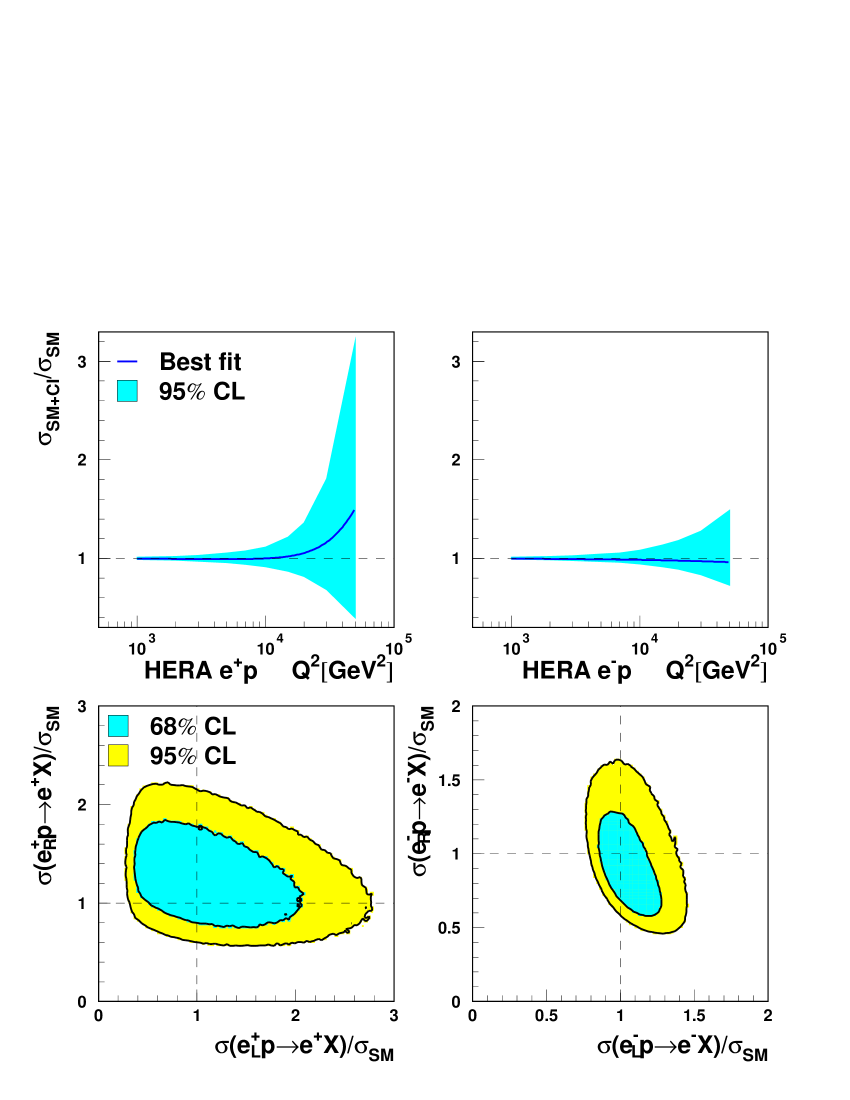
Figure 8: The 95% CL limit band on the ratio of predicted to the Standard Model cross-section for $e^{+}p$ and $e^{-}p$ NC DIS scattering at HERA (upper plots) and the 68% and 95% CL contours for the possible deviations for scattering of right- and left-handed electrons and positrons at $Q^{2}=$30,000 GeV² (lower plots). The limits are calculated using the general contact interaction model.

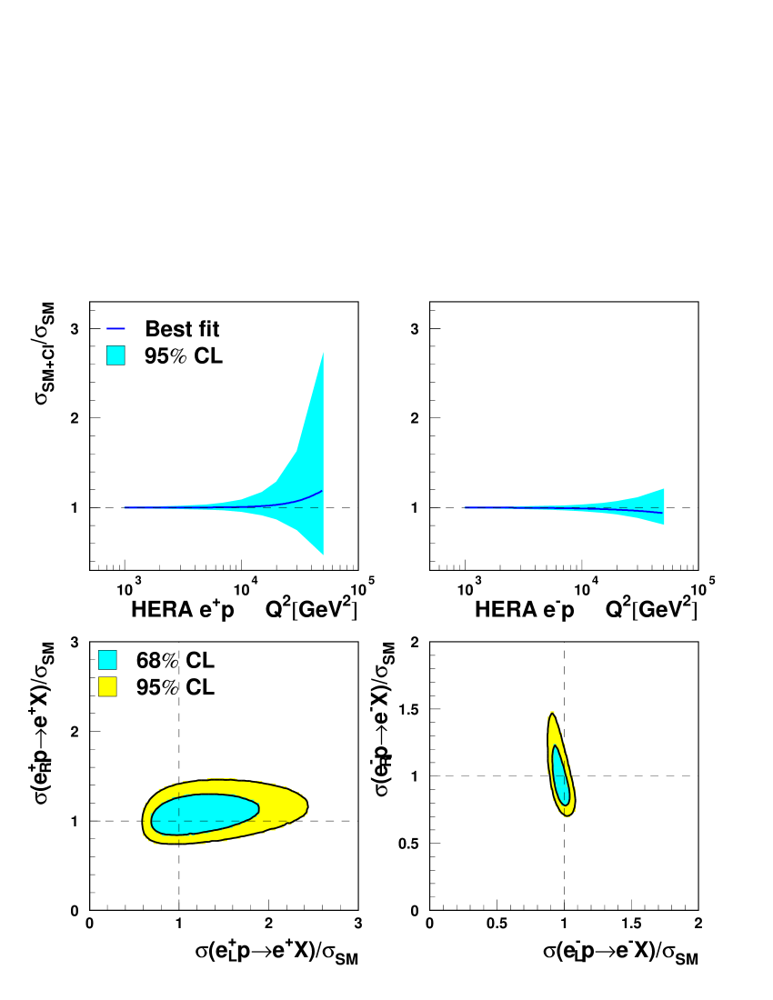
Figure 9: The 95% CL limit band on the ratio of predicted to the Standard Model cross-section for $e^{+}p$ and $e^{-}p$ NC DIS scattering at HERA (upper plots) and the 68% and 95% CL contours for the possible deviations for scattering of right- and left-handed electrons and positrons at $Q^{2}=$30,000 GeV² (lower plots). The limits are calculated using the SU(2) contact interaction model with family universality.

For the $e^{+}p$ NC DIS the uncertainty of these predictions is very big, although the nominal predictions of both models are above the Standard Model. The Standard Model prediction is well within the 95% confidence level band. For the general model, the increase in the $e^{+}p$ NC DIS cross-section at HERA by up to about 80% at $Q^{2}$ of 30,000 GeV² would still be consistent with current experimental data. For the SU(2) model the corresponding limit is 63%. It turns out that the best statistical sensitivity (in single measurement) to possible contact interaction effects is obtained when considering the number of events measured for $Q^{2}\;>$ 15,000 GeV². The allowed increase in the integrated $e^{+}p$ NC DIS cross-section is about 40% for the general model and about 30% for the SU(2) model. In order to reach the level of statistical precision, which would allow them to confirm possible discrepancy of this size, HERA experiments would have to collect $e^{+}p$ luminosities of the order of 100-200 pb^-1 (depending on the model). This will be possible after the HERA upgrade planned for year 2000.

Constraints on the possible deviations from the Standard Model predictions are much stronger in case of $e^{-}p$ NC DIS. This is because the Standard Model cross-section itself is higher, and also because different contact interaction coupling combinations contribute. It is interesting to notice that the possible cross-section increase for $e^{+}p$ NC DIS, which is suggested by global fit results, corresponds to decrease in the NC DIS cross-section for $e^{-}p$. For the general model, deviations larger than about 20% are excluded for $Q^{2}>$15,000 GeV², whereas for the SU(2) model with family universality the limit goes down to about 7%. When compared with the predicted statistical precision of the future HERA data, this indicates that it will be very hard to detect contact interactions in the future HERA $e^{-}p$ running. For the general model the required luminosity is of the order of 400 pb^-1.

However, the HERA ”discovery window” can be visibly enlarged if we consider scattering of polarised electrons and/or positrons. The 68% and 95% CL contours for the allowed deviations for scattering of right- and left-handed electrons or positrons are included in Figures 8 (for general model) and 9 (for SU(2) model), at $Q^{2}=$30,000 GeV². In both cases, the cross-section deviations for $e^{+}_{L}p$ and $e^{-}_{R}p$ scattering are less constrained than in case of $e^{+}_{R}p$ and $e^{-}_{L}p$, respectively. For the general model possible deviations for both left- and right-handed projectiles are significantly higher than in the unpolarised case. However, for the SU(2) model, constraints significantly weaker than in the unpolarised case are obtained only for $e^{+}_{L}p$ and $e^{-}_{R}p$ scattering. In both models deviations of up to about 50% are still allowed for $e^{+}_{L}p$ scattering at $Q^{2}>$15,000 GeV², assuming 60% polarisation of the positron beam. To observe effects of this size it would be enough to collect luminosity of the order of 70-80 pb^-1. For $e^{-}_{R}p$ scattering maximum allowed deviations are 28% and 19%, for the general and SU(2) models respectively. It means that with 60% longitudinal $e^{-}_{R}$ polarisation it would be possible to observe significant deviations from Standard Model predictions already for luminosities of the order of 120 pb^-1 (for the general model). Unfortunately, polarisation can result in significantly higher systematic uncertainties of the Standard Model predictions, which was not considered here.

Since the only visible inconsistency between data and the Standard Model is observed in the Charged Current sector (for models assuming $SU(2)_{L}\times U(1)_{Y}$ universality), the interesting question is whether any effect can be observed in high $Q^{2}$ CC DIS at HERA. It turns out that the possible effect is far beyond the HERA sensitivity. The “best” $\eta^{CC}$ value (resulting from the SU(2) model fit) corresponds to a decrease in the CC DIS cross-section at HERA not greater than 2% within the accessible $Q^{2}$ range, and a decrease exceeding 5% is excluded at 95% CL. At the same confidence level, any increase in the cross-section by a similar amount is excluded.

Model predictions for both the total hadronic cross-section at electron-positron collider (LEP or NLC) and Drell-Yan lepton pair production cross-section at the Tevatron are shown in Figures 10 and 11, for the general contact interaction model and the SU(2) model, respectively. For $e^{-}e^{+}\rightarrow q\bar{q}$ at $\sqrt{s}$ above about 300 GeV upper cross-section limits obtained from both contact interaction models increase rapidly. Cross-section deviations up to a factor of 3 are allowed for $\sqrt{s}\sim$500 GeV. Unfortunately, this energy range will be accessible only in the Next Linear Collider experiment(s). LEP will not go beyond $\sqrt{s}\sim$200 GeV: at this energy the possible deviations from the Standard Model are only about 8%, which makes possible discovery very difficult.

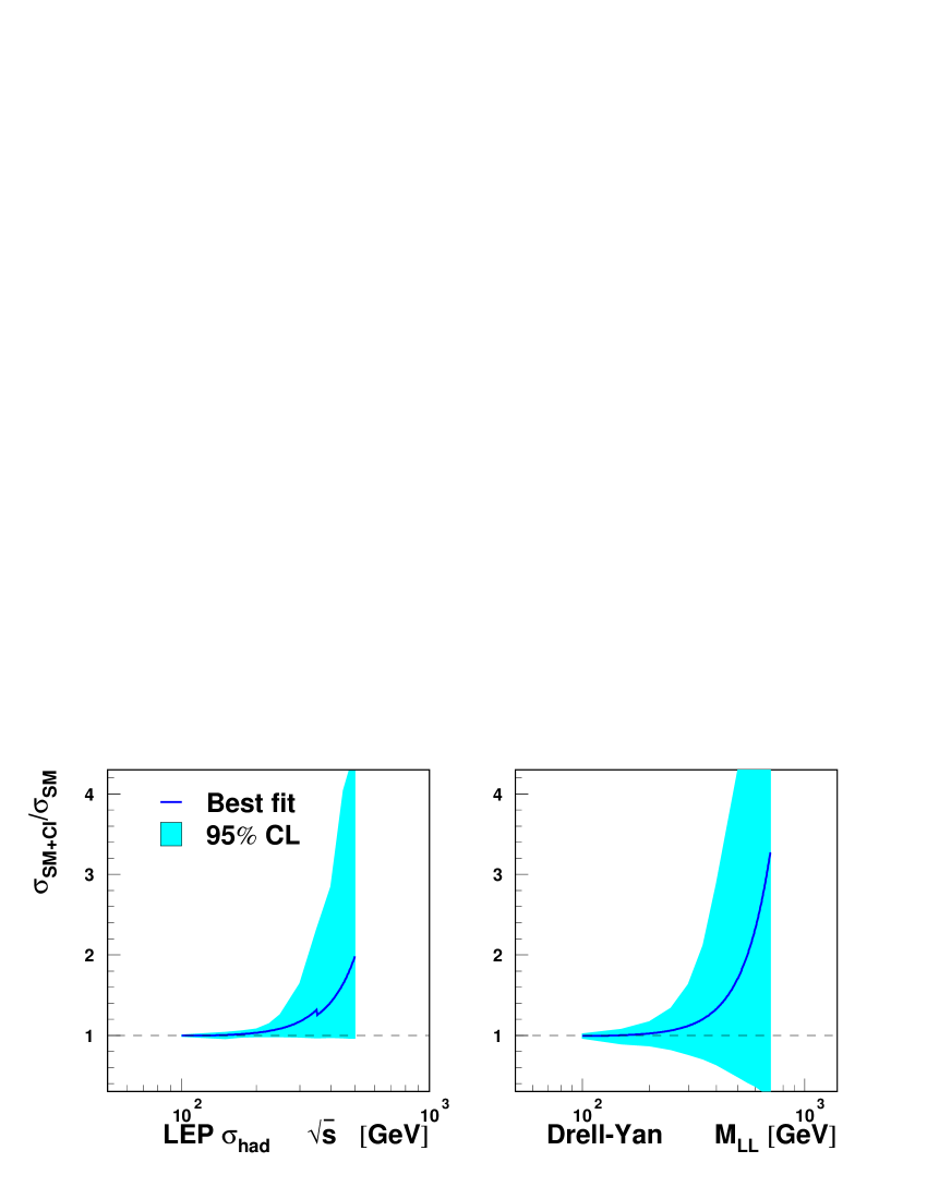
Figure 10: Left: the 95% CL limit band on the ratio $\sigma_{SM+CI}/\sigma_{SM}$, where $\sigma_{SM}$ is the Standard Model total hadronic cross-section at LEP/NLC and $\sigma_{SM+CI}$ is the cross-section calculated in the general contact interaction model; Right: the same ratio for the Drell-Yan lepton pair production at the Tevatron.

	SM	Allowed range on 95% C.L.
	Value	General		Model with		SU(2) model
	(LO)	model		family univ.		w. fam. univ.
$R_{b}$	0.159	0.147 -	0.161	0.137 -	0.180	0.139 -	0.179
$R_{c}$	0.262	0.242 -	0.266	0.230 -	0.294	0.232 -	0.291
$A^{b}_{FB}$	0.601	-		0.345 -	0.750	0.431 -	0.732
$A^{c}_{FB}$	0.668	-		0.469 -	0.750	0.551 -	0.738

Table 7: Leading order Standard Model prediction and the allowed range (on 95% CL) for the heavy quark production ratios and forward-backward asymmetries, for $e^{+}e^{-}$ annihilation at $\sqrt{s}$=200 GeV, in different contact interaction models.

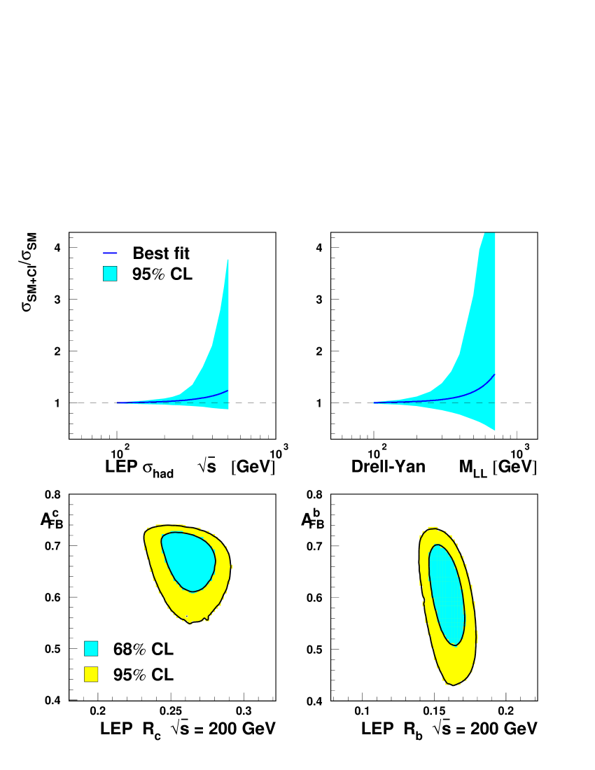
Figure 11: Upper left: the 95% CL limit band on the ratio $\sigma_{SM+CI}/\sigma_{SM}$, where $\sigma_{SM}$ is the Standard Model total hadronic cross-section at LEP/NLC and $\sigma_{SM+CI}$ is the cross-section calculated in the SU(2) contact interaction model; Upper right: the same ratio for the Drell-Yan lepton pair production at the Tevatron; Below: the 68% and 95% CL contours for the allowed values of the forward-backward asymmetries and the quark production fractions for $c$ and $b$ quark production at LEP, at $\sqrt{s}$=200 GeV.

However, significant deviations from Standard Model predictions are still possible for heavy quark production ratios $R_{c}$ and $R_{b}$, and for the forward-backward asymmetries $A^{c}_{FB}$ and $A^{b}_{FB}$. The 68% and 95% CL contours for the values of the forward-backward asymmetry versus the quark production fraction, allowed within the SU(2) model for $c$ and $b$ quark production at $\sqrt{s}$=200 GeV are included in Figure 11. Allowed ranges for $R_{c}$, $R_{b}$, $A^{c}_{FB}$ and $A^{b}_{FB}$ at $\sqrt{s}$=200 GeV, for different contact interaction models considered, are summarised in Table 7. For the general model, in which contact interactions are limited to the first quark generation only, variations of $R_{b}$ and $R_{c}$ are still possible, due to the possible changes in $u\bar{u}$ and $d\bar{d}$ production cross-sections. However, parton level forward-backward asymmetries $A^{c}_{FB}$ and $A^{b}_{FB}$ do not depend on contact interaction couplings in this model. Therefore limits for $A^{c}_{FB}$ and $A^{b}_{FB}$ are not reported for the general model. Heavy quark observables considered here are least constrained for the model with family universality. Large effects are still possible in this model for both production fractions and asymmetries. Deviations up to about 13% are possible for $R_{b}$ and $R_{c}$. Least constrained by the existing experimental data is the forward-backward asymmetry for the $b\bar{b}$ production $A^{b}_{FB}$, where deviations from the Standard Model prediction by up to 40% are still possible. Note that for the general model $R_{b}$ and $R_{c}$ are 100% correlated, whereas for models with the family universality they are 100% anti-correlated.

It seems that the best place to study contact interactions in the nearest future is the Tevatron, which should run again after being upgraded in the year 2000. If there is any ”new physics” corresponding to the contact interaction model it is very likely to show up in Drell-Yan lepton pair production for masses above 200-300 GeV. Moreover, upper limits on possible deviations from the Standard Model predictions are much higher than in case of HERA and LEP/NLC. For $M_{ll}=$500 GeV, which should be easily accessible with increased luminosity, cross-section deviations up to a factor of 5 are still not excluded.

Upper limits on the cross-section deviations from the Standard Model predictions, derived on 95% confidence level in different contact interaction models are summarised in Table 8.

		Limits on $\Delta\sigma/\sigma_{SM}$ [%]
Reaction	Energy	General	Model with	SU(2) model
	scale	model	family univ.	w. family univ.
$e^{+}p$ NC DIS	$Q^{2}$=10000 GeV2	11	10	9
$\sqrt{s}=$318 GeV	$Q^{2}$=20000 GeV2	36	30	28
	$Q^{2}$=30000 GeV2	81	65	63
	$Q^{2}$=50000 GeV2	220	180	170
$e^{-}p$ NC DIS	$Q^{2}$=10000 GeV2	8	4	3
$\sqrt{s}=$318 GeV	$Q^{2}$=20000 GeV2	18	8	7
	$Q^{2}$=30000 GeV2	28	13	11
	$Q^{2}$=50000 GeV2	49	26	21
$e^{-}e^{+}\rightarrow q\bar{q}$	$\sqrt{s}$=175 GeV	5	5	6
	$\sqrt{s}$=200 GeV	8	8	8
	$\sqrt{s}$=225 GeV	14	13	11
	$\sqrt{s}$=250 GeV	26	24	16
	$\sqrt{s}$=300 GeV	65	61	35
	$\sqrt{s}$=400 GeV	185	185	110
$p\bar{p}\rightarrow l^{+}l^{-}X$	$M_{ll}$=200 GeV	17	12	12
$\sqrt{s}=$ 1800 GeV	$M_{ll}$=300 GeV	64	55	38
	$M_{ll}$=400 GeV	190	185	95
	$M_{ll}$=500 GeV	440	450	210

Table 8: Upper limits (on 95% CL) on cross-section deviations from the Standard Model predictions in different contact interaction models. Considered are $e^{+}p$ and $e^{-}p$ scattering at HERA, total hadronic cross-section at LEP/NLC and Drell-Yan lepton pair production at the Tevatron, as indicated in the table.

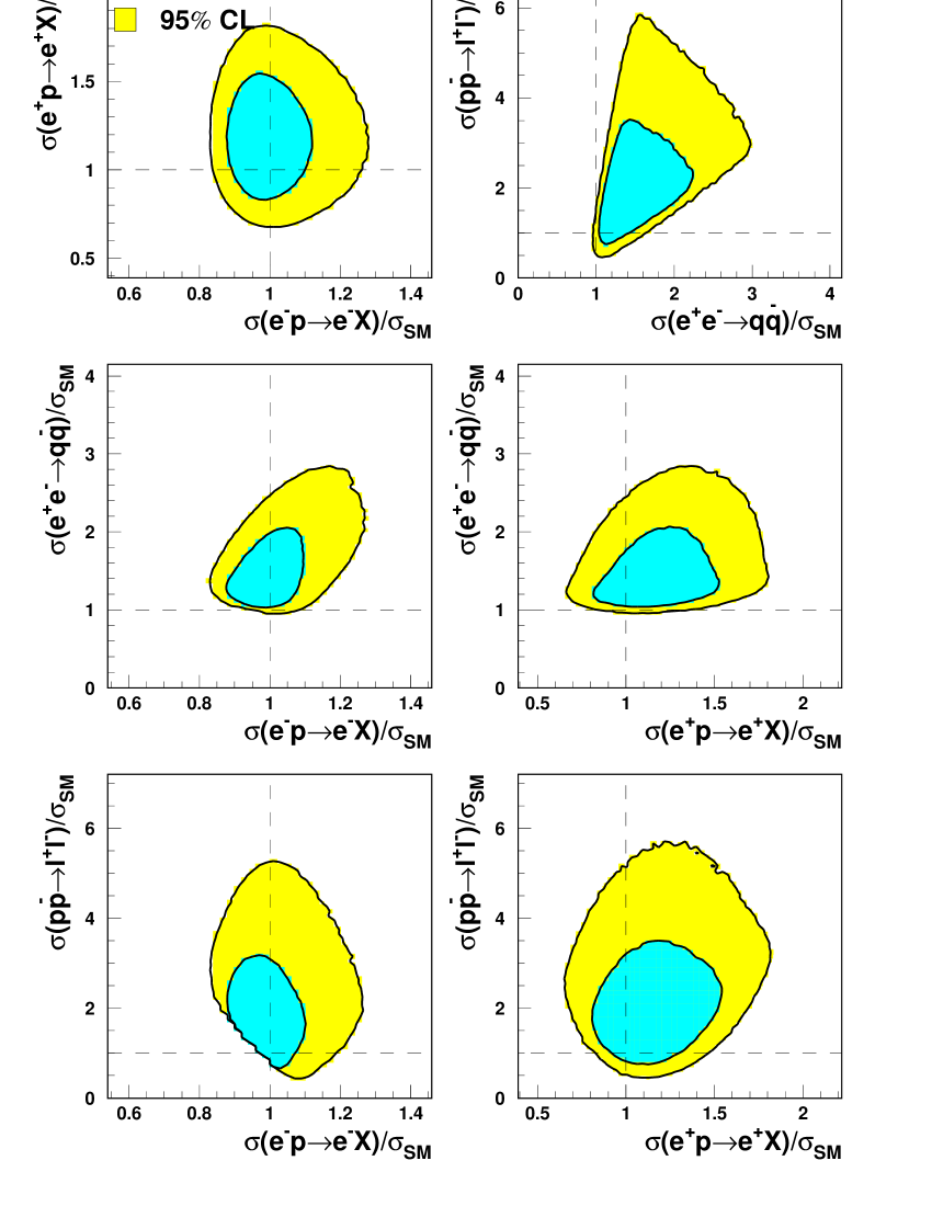
Figure 12: The 68% and 95% CL contours for the possible deviation from the Standard Model predictions, for different combinations of measurements. Considered are: $e^{+}p$ and $e^{-}p$ NC DIS cross-section at HERA, at $Q^{2}$ = 30,000 GeV², total $e^{+}e^{-}\rightarrow q\bar{q}$ cross-section at $\sqrt{s}$ = 400 GeV and Drell-Yan lepton pair production cross-section at the Tevatron, at $M_{ll}$ = 500 GeV, as indicated on the plot. The limits are calculated using the general contact interaction model.

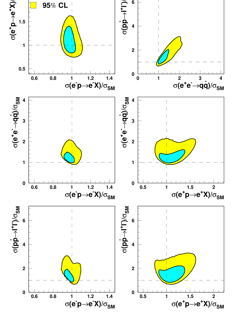
Figure 13: The 68% and 95% CL contours for the possible deviation from the Standard Model predictions, for different combinations of measurements. Considered are: $e^{+}p$ and $e^{-}p$ NC DIS cross-section at HERA, at $Q^{2}$ = 30,000 GeV², total $e^{+}e^{-}\rightarrow q\bar{q}$ cross-section at $\sqrt{s}$ = 400 GeV and Drell-Yan lepton pair production cross-section at the Tevatron, at $M_{ll}$ = 500 GeV, as indicated on the plot. The limits are calculated using the SU(2) contact interaction model with family universality.

When considering possible future discoveries at high-energy experiments, it is also interesting to study the relation between effects observed at different experiments. The 68% and 95% CL contours for the sizes of the allowed deviation from the Standard Model predictions, for different measurement combinations, are shown in Figures 12 and 13, for the general contact interaction model and for the SU(2) model with family universality, respectively. In both cases, clear correlation is observed between the Drell-Yan cross-section deviation at the Tevatron and the hadronic $e^{+}e^{-}$ cross-section at LEP/NLC. Possible cross-section increase at the Tevatron has to be accompanied by the increase in the hadronic cross-section at LEP/NLC. Similar correlation is observed between the hadronic $e^{+}e^{-}$ cross-section at LEP/NLC and $e^{+}p$ NC DIS cross-section at HERA for SU(2) model. Another interesting observation is that the possible decrease in the $e^{-}p$ NC DIS cross-section at HERA should be related to the increase in both Tevatron and LEP/NLC cross-section. In other cases correlations between different measurements are weak. This shows that contact interaction searches at LEP, the Tevatron and HERA are, to large extent, independent. Data from all types of experiments are necessary to constraint contact interaction model in general case.

7 Summary

Data from HERA, LEP, the Tevatron and low energy experiments were used to constrain electron-quark contact interactions. The contact interaction mass scale limits obtained for different one-parameter models range from 5.1 to about 18 TeV. Using the most general approach, in which all couplings to are allowed to vary independently, any contact interactions with mass scale below 2.1 TeV are excluded at 95% CL. This limit can be raised to 3.1 TeV by assuming $SU(2)_{L}\times U(1)_{Y}$ and quark/lepton family universality. There is a slight hint on possible “new physics” in the Charged Current sector (related to Neutral Current contact interactions by $SU(2)_{L}\times U(1)_{Y}$ universality), where the discrepancy between data and the Standard Model is at the $2\sigma$ level. The mass scale of new Charged Current interactions suggested by the data is of the order of 10 TeV. However, this effect - if real - would have negligible impact on predictions for future collider results.

The limits on possible effects to be observed in future HERA, LEP and Tevatron running are estimated. Possible deviations from the Standard-Model predictions for total hadronic cross-section at LEP and $e^{-}p$ scattering cross-section at HERA, are already strongly limited by existing data. However, improved experimental sensitivity to new interactions should result from the measurement of heavy quark production ratios and asymmetries at LEP, as well as from polarised electron scattering at HERA. Sizable effects are still not excluded for $e^{+}p$ NC DIS at HERA and the required statistical precision of the data should be accessible after HERA upgrade. The best ”discovery potential” seems to come from future Tevatron running, where significant deviations from the Standard Model predictions are still allowed. For Drell-Yan lepton pair production cross-section deviations at $M_{ll}$=500 GeV up to a factor of 5 are still not excluded. However, all experiments should continue to analyse their data in terms of possible new electron-quark interactions, as constraints resulting from different experiments are, to large extent, complementary.

Appendix A Interpretation of the probability function

In this appendix a simple ”toy model” is used to demonstrate that the probability function, as introduced in section 4, should not be treated as the probability distribution for $\vec{\eta}$.

Let us consider a model with N independent couplings. Assume that all data considered in the analysis are in perfect agreement with the Standard Model and that the resulting probability function is

$${\cal P}(\vec{\eta}) = \frac{1}{(\sqrt{2\pi}\sigma)^{N}}\cdot\exp\left(-\frac{\vec{\eta}^{\;2}}{2\sigma^{2}}\right)$$

where $\vec{\eta}^{\;2}=\eta_{1}^{2}+...+\eta_{N}^{2}$ and the distribution width $\sigma$ is taken to be the same for all couplings. The Standard Model gives the best description of the data, corresponding to the maximum value of ${\cal P}(\vec{\eta})$.

Consider the cross-section deviation from the Standard Model prediction, which is of the form

$$r(\vec{\eta}) = \frac{\sigma(\vec{\eta})}{\sigma_{SM}}\;=\;(1+\vec{\eta}^{\;2})$$

If ${\cal P}(\vec{\eta})$ is taken as a probability distribution, then the probability distribution for $r$ should be calculated from equation (18). After integrating over the coupling space we obtain:

$$P(r) = \frac{(r-1)^{\frac{N}{2}-1}}{2^{\frac{N}{2}}\sigma^{N}\Gamma(\frac{N}{2})}\cdot\exp\left(-\frac{r-1}{2\sigma^{2}}\right)$$

The shape of $P(r)$ corresponds to that of the $\chi^{2}$ distribution for N degrees of freedom. For $N\leq 2$, $P(r)$ has a maximum for $r=1$, i.e. for the Standard Model expectation. However, for models with $N\geq 3$ parameters, the maximum of $P(r)$ is shifted towards $r>1$ and the probability of the Standard Model solution $P(r=1)=0$. This results is incompatible with our initial assumption that all data are in perfect agreement with the Standard Model.

The above calculation, based on the formula (18), is not correct because it assumes that ${\cal P}(\vec{\eta})$ is the probability distribution for $\vec{\eta}$. We can treat ${\cal P}(\vec{\eta})$ as the probability distribution only if we assume that $\vec{\eta}$ has a flat prior distribution. This assumption justifies limit setting procedure described in section 4.6 (formula (22)). However, it does not justify variable transformation from $\vec{\eta}$ to $r$ (resulting from equation (18)), as the prior distribution for the new variable does not need to be flat. Instead, one should try to define $P(r)$ in the same way as ${\cal P}(\vec{\eta})$, i.e. as the probability that our data come from the model predicting deviation $r$. This approach results in formula (19). For our toy model the probability of observing deviations from the Standard Model predictions is

$$P(r) = \exp\left(-\frac{(r-1)}{2\sigma^{2}}\right)$$

where the normalisation condition (20) has been imposed. The result does not depend on the number of free model parameters and the most probable model is the one predicting no deviation from the Standard Model (taking into account that $r\geq 1$).

References

- [1] The H1 Collaboration, C.Adloff et al., Z. Phys. C74, (1997) 191.
- [2] The ZEUS Collaboration, J.Breitweg et al., Z. Phys. C74, (1997) 207.
- [3] The H1 Collaboration, ICHEP’98 paper #533.
- [4] The ZEUS Collaboration, J.Breitweg et al., DESY 99-056, submitted to Euro.Phys.J. C.
-
[5]
V. Barger, K. Cheung, K. Hagiwara, D. Zeppenfeld,
Phys. Rev. D57, (1998) 391.
D. Zeppenfeld, K.Cheung, MADPH-98-1081, hep-ph/9810277. -
[6]
R.Rückl, Phys. Lett. B129, (1983) 363.
E.Eichten, K.Lane, M.Peskin, Phys. Rev. Lett. 50, (1983) 811. - [7] P.Haberl, F.Schrempp, H.-U.Martyn, Proc. Workshop Physics at HERA (ed. W. Buchmüller, G.Ingelman, Hamburg 1991) Vol. 2, pg. 1133.
- [8] The H1 Collaboration, S. Aid et al., Phys. Lett. B353, (1995) 578.
- [9] The ZEUS Collaboration, ICHEP’96 paper pa04-036.
- [10] The ZEUS Collaboration, ICHEP’98 paper #751.
- [11] The ZEUS Collaboration, J.Breitweg et al., DESY-99-058, submitted to Euro.Phys.J. C.
-
[12]
The CDF Collaboration, F.Abe et al.,
Phys. Rev. Lett 79, (1997) 2198.
The CDF Collaboration, F.Abe et al., Phys. Rev. D59, (1999) 052002. -
[13]
The D0 Collaboration, Fermilab-CONF-98-273-E.
The D0 Collaboration, Fermilab-PUB-98-391-E. -
[14]
The ALEPH Collaboration, CERN-EP/99-042.
The ALEPH Collaboration, ALEPH-99-018. - [15] The DELPHI Collaboration, ICHEP’98 paper #439.
-
[16]
The DELPHI Collaboration, ICHEP’98 paper #441.
The DELPHI Collaboration, ICHEP’98 paper #643. -
[17]
The L3 Collaboration, Phys. Lett. B370, (1996) 195.
The L3 Collaboration, Phys. Lett. B407, (1997) 361.
The L3 Collaboration, L3-Note-2227, ICHEP’98 paper #484.
The L3 Collaboration, L3-Note-2304, ICHEP’98 paper #510. -
[18]
The OPAL Collaboration, Euro. Phys. J. C2, (1999) 441.
The OPAL Collaboration, Euro. Phys. J. C6, (1999) 1.
The OPAL Collaboration, OPAL-PN-372 (1999). - [19] Ian Tomalin, private communication.
-
[20]
The OPAL Collaboration, OPAL-PN-348, ICHEP’98 paper #268.
The OPAL Collaboration, OPAL-PN-380 (1999). - [21] Gi-Chol Cho, K. Hagiwara, S. Matsumoto, Euro. Phys. J. C5, (1998) 155.
- [22] C.S. Wood et al., Science 275, (1997) 1759.
- [23] S.A. Blundell, J. Sapirstein, W.R. Johnson, Phys. Rev D45, (1992) 1602.
- [24] Review of Part. Phys., Euro. Phys. J. C3 (1998).
-
[25]
P.A. Vetter et al., Phys. Rev. Lett. 74, (1995) 2658.
N.H. Edwards et al., Phys. Rev. Lett. 74, (1995) 2654. -
[26]
Y. Prescott et al., Phys. Lett. B84, (1979) 524.
K. Hagiwara, D. Haidt, C.S. Kim, S. Matsumoto, Z. Phys. C64, (1994) 559.
K. Hagiwara, D. Haidt, C.S. Kim, S. Matsumoto, Z. Phys. C68, (1995) 352(E). - [27] P.A. Souder et al., Phys. Rev. Lett. 65, (1990) 694.
- [28] W. Heil et al., Nucl. Phys. B327, (1989) 1.
- [29] A. Argento et al., Phys. Lett. B120, (1983) 245.
- [30] G.L. Fogli, D. Haidt, Z. Phys. C40, (1988) 379.
- [31] K. McFarland et al., Euro. Phys. J. C1, (1998) 509.
- [32] K. McFarland et al., hep-ex/9806013.
- [33] G. Altarelli, G.F. Giudice, M.L. Mangano, Nucl. Phys. B506, (1997) 29.
- [34] K. Hagiwara, S. Matsumoto, Phys. Lett. B424, (1998) 362.
-
[35]
W.J.Marciano, A.Sirlin, Phys. Rev. Lett. 71, (1993) 3629.
M.Finkemeier, Phys. Lett. B387, (1996) 391. - [36] Physics at LEP2 (ed. G.Altarelli, T.Sjöstrand, F.Zwirner, CERN 96-01) Vol. 1, pg. 207.
- [37] F.A.Berends, W.L.van Neerven, G.J.H.Burgers, Nucl. Phys. B297, (1988) 429.
- [38] CERN Program Library entry D506.