QUARK CONFINEMENT AND THE HADRON SPECTRUM

Abstract

These lectures contain an introduction to the following topics:

• Phenomenology of the hadron spectrum.

• The static Wilson loop in perturbative and in lattice QCD. Confinement and the flux tube formation.

• Non static properties: effective field theories and relativistic corrections to the quarkonium potential.

• The QCD vacuum: minimal area law, Abelian projection and dual Meissner effect, stochastic vacuum.

Dedicated to the 60th birthday of Dieter Gromes

1 Introduction

Quarks appear to be confined in nature. This means that free quarks have not been detected so far but only hadrons, their bound states. Therefore, predictions of the hadron spectrum are an explicit and direct test of our understanding of the confinement mechanism as a result of the low energy dynamics of QCD. In these lectures we will focus on heavy quark bound states and for simplicity we will only treat the quark-antiquark case i.e. the mesons. Indeed, also in order to extract the Cabibbo–Kobayashi–Maskawa matrix elements and to study CP violation from the experimental decay rate of heavy mesons, hadronic matrix elements are needed. It is reasonable to expect that to this aim the somewhat simpler matching of the theoretical prediction for the spectrum to experiment has to be previously established. Moreover, we need to achieve some understanding of the bound state dynamics in QCD in order to make reliable identifications of the gluonic degrees of freedom in the spectrum (hybrids, glueballs). All this is relevant to the programme of most of the accelerators machines, Godfrey et al. (1998). From a more general point of view, the issue about the consequences of a nontrivial vacuum structure and the nonperturbative definition of a field theory are questions that overlap with the domain of supersymmetric and string theories.

These lectures are quite pedagogical and introductory and contain several illustrative exercises. The interested reader is referred for details to the quoted references.

The plan of the lectures is the following one. In Secs. 2 and 3 we give a brief overview on the hadron spectrum and on the phenomenological models devised to explain it. The nonperturbative phenomenological parameter $\sigma$ is introduced and connected to the Regge trajectories as well as to the string models. In Sec. 4 we evaluate perturbatively and nonperturbatively (via lattice simulations) the static Wilson loop. We discuss the area law behaviour and the flux tube formation as signals of confinement. In Sec. 5 we summarize some existing model independent results on the heavy quark interaction. QCD effective field theories are introduced. In Sec. 6 we connect confinement to the structure of the QCD vacuum. We study with some detail the Minimal Area Law model. We discuss the Abelian Higgs model and the Dual Meissner effect and introduce the idea of ’t Hooft Abelian projection. We list some of the results obtained on the lattice with partial gauge fixing. Finally we briefly review two models of the QCD vacuum: Dual QCD and the Stochastic Vacuum Model. Each section is supplemented with some exercises. We tried to be as self-contained as possible reporting all the relevant definitions and the basic concepts.

2 The Hadron Spectrum

The meson and the baryon resonances together with an introduction to the quark model have been discussed at this school by Jim Napolitano. Since these lectures are mainly concerned with the quark confinement mechanism, they contain only a general overview on the spectrum pointing out its relevant features.

b

Figure 1: The spectrum of the lightest mesons labeled by $({\rm spin})^{\rm parity}$.

Let us concentrate on the meson spectrum as given in Figs. 1-3. In principle, one should be able to explain and predict it only by means of the QCD Lagrangian

$$L=-{1\over 4}F^{(a)}_{\mu\nu}F^{(a)\mu\nu}+i\sum_{q=1}^{N_{f}}\bar{\psi}_{q}^{i}\gamma^{\mu}(D_{\mu})_{ij}\psi_{q}^{j}-\sum_{q=1}^{N_{f}}m_{q}\bar{\psi}_{q}^{i}\psi_{q}^{i}$$ (1)

where

$$F_{\mu\nu} \equiv\partial_{\mu}A_{\nu}-\partial_{\nu}A_{\mu}+ig[A_{\mu},A_{\nu}]$$

$$(D_{\mu})_{ij} \equiv\delta_{ij}\partial_{\mu}+ig{\lambda^{a}_{ij}\over 2}A^{a}_{\mu}\,;\quad\quad\qquad A_{\mu}\equiv A_{\mu}^{a}{\lambda_{a}\over 2}\quad a=1,\dots,8.$$ (2)

$\psi^{j}_{q}$ are the quark fields of flavour $q=1,\dots,6=N_{f}$ and colour $j=1,\dots,3$, $m_{q}$ the (current) quark masses and $\lambda^{a}$ the Gell-Mann matrices of $SU(3)$. However, if we proceed to calculate the spectrum from this Lagrangian using the familiar tool of a perturbative expansion in the coupling constant $g$, we get no match with the experimental data presented in Figs. 1-3. This is a consequence of the most relevant feature of the Lagrangian (1): asymptotic freedom (Gross and Wilczek (1973), Politzer (1973)). The coupling constant ($\alpha_{\rm s}\equiv g^{2}/4\pi$) vanishes in the infinitely high energy region and grows uncontrolled in the infrared energy region:

$${d\,\alpha_{\rm s}(\mu)\over d\log\mu^{2}}\equiv\beta(\alpha_{\rm s})=-\alpha_{\rm s}\left(\beta_{0}{\alpha_{\rm s}\over 4\pi}+\beta_{1}\left({\alpha_{\rm s}\over 4\pi}\right)^{2}+\cdots\right)$$ (3)

where $\beta_{0}=11-2/3N_{f}>0$. As a consequence, a perturbative treatment is expected to be reliable in QCD only when the energy $\mu$ is large compared to $\Lambda_{QCD}$, which is the infrared energy scale defined by Eq. (3). The point is that the relevant energies in a quark bound state are in most cases of the order of the naturally occurring scale of 1 fm ($\simeq\Lambda_{QCD}^{-1}$), the average hadron size. The only exception are the mesons made up with top quarks. Unfortunately, they have not enough time to exist!

b

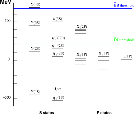
Figure 2: The experimental heavy meson spectrum ($b\bar{b}$ and $c\bar{c}$) relative to the spin-average of the $\chi_{b}(1P)$ and $\chi_{c}(1P)$ states.

The masses appearing in the Lagrangian are the so-called “current masses” and fall into two categories: light quark masses $m_{u}=1.5\div 5$ MeV, $m_{d}=3\div 9$ MeV, $m_{s}=60\div 170$ MeV ($m_{u}$, $m_{d}\ll\Lambda_{QCD}$ and $m_{s}\sim\Lambda_{QCD}$) and heavy quark masses $m_{c}=1.1\div 1.4$ GeV, $m_{b}=4.1\div 4.4$ GeV, $m_{t}=173.8\pm 5.2$ GeV ($m_{c},m_{b},m_{t}\gg\Lambda_{QCD}$). The spectrum should be obtained from the QCD Lagrangian with these values of the masses. However, in the light quark sector, spontaneous chiral symmetry breaking and non-linear strongly coupled effects cooperate in a highly non trivial way. Indeed, it is peculiar of QCD that, due to confinement, the quark masses are not physical, i.e. directly measurable quantities. Therefore, it turns out to be useful, in order to make phenomenological predictions, to introduce the so-called constituent quark masses, containing the current masses as well as mass corrections also due to confinement effects. These constituent masses can be defined, for example, using the additivity of the quark magnetic moments inside a hadron or using phenomenological potential models to fit the spectrum. For quarks heavier than $\Lambda_{QCD}$ the difference between current and constituent masses is not quite relevant.

In the framework of the constituent quark model the meson states are classified as follows. For equal masses the quark and the antiquark spins combine to give the total spin ${\bf S}={\bf S}_{1}+{\bf S}_{2}$ which combines with the orbital angular momentum ${\bf L}$ to give the total angular momentum ${\bf J}$. The resulting state is denoted by $n^{2S+1}L_{J}$ where $n-1$ is the number of radial nodes. As usual, to $L=0$ is given the name $S$, to $L=1$ the name $P$, to $L=2$ the name D and so on. The resonances are classified via the $J^{PC}$ quantum numbers, $P=(-1)^{L+1}$ being the parity number and $C=(-1)^{L+S}$ the C-parity.

b

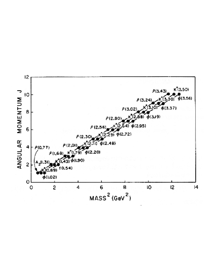
Figure 3: The Regge trajectories for the $\rho$, $K^{*}$ and $\phi$. From Godfrey et al. (1985).

Light mesons (as well as baryons) of a given internal symmetry quantum number but with different spins obey a simple spin ($J$)-mass ($M$) relation. They lie on a Regge trajectory

$$J(M^{2})=\alpha_{0}+\alpha^{\prime}M^{2}$$ (4)

with $\alpha^{\prime}\simeq 0.8-0.9\,{\rm GeV}^{-2}$, see Fig. 3. Up to now, free quarks have not been detected. The upper limit on the cosmic abundance of relic quarks, $n_{q}$, is $n_{q}/n_{p}<10^{-27}$, $n_{p}$ being the abundance of nucleons, while cosmological models predict $n_{q}/n_{p}<10^{-12}$ for unconfined quarks. The fact that no free quarks have been ever detected hints to the property of quark confinement. Hence, the interaction among quarks has to be so strong at large distances that a $q\bar{q}$ pair is always created when the quarks are widely separated. From the data it is reasonable to expect that a quark typically comes accompanied by an antiquark in a hadron of mass $1\,{\rm GeV}$ at a separation of 1 fm ($\simeq\Lambda_{QCD}^{-1}$). This suggests that between the quark and the antiquark there is a linear energy density (called string tension) of order

$$\sigma={\Delta E\over\Delta r}\simeq 1{{\rm GeV}\over{\rm fm}}\simeq 0.2\,{\rm GeV}^{2}.$$ (5)

The evidence for linear Regge trajectories (see Fig. 3) supports this picture. A theoretical framework is provided by the string model, Nambu (1974). In this model the hadron is represented as a rotating string with the two quarks at the ends. The string is formed by the chromoelectric field responsible for the flux tube configuration and for the quark confinement (see Fig. 4), Buchmüller (1982). Upon solution of the Exercise 2.1, the reader can verify that it is possible to establish the relation

$$\alpha^{\prime}={1\over 2\pi\sigma}$$ (6)

between the slope of the Regge trajectories and the string tension. The string tension $\sigma$ emerges as a key phenomenological parameter of the confinement physics.

b

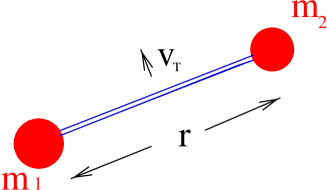
Figure 4: Picture of the quark-antiquark bound state in the string model.

From the light mesons spectrum of Fig. 1 it is evident that

• the separations between levels are considerably larger than the mesons masses $\Longrightarrow$ they are truly relativistic bound states;

• the splitting between the pseudoscalar $\pi$ and the vector $\rho$ mesons is so large to be anomalous $\Longrightarrow$ it is due to the Goldstone boson nature of the $\pi$.

Therefore, understanding the light meson spectrum means to solve a relativistic many-body bound state problem where confinement is strongly related with the spontaneous breaking of chiral symmetry. Since the target of these lectures is to gain some understanding of the confinement mechanism in relation to the spectrum, we will try to separate problems and to consider first the spectrum of mesons built by heavy valence quarks only. In this case we have still bound states of confined quarks, however, due to the large mass of the quarks involved, we can hope to treat relativistic and many-body (i.e. quark pair creation effects) contributions as corrections. The problem simplifies remarkably if we consider mesons made up by two valence heavy quarks ($b\bar{b}$, $c\bar{c}$, $b\bar{c}$, …) i.e. quarkonium.

2. Exercises

• Consider two massless and spinless quarks connected by a string of length $R$ rotating with the endpoints at the speed of light, so that each point at distance $r$ from the centre has the local velocity $v/c=2r/R$. Recalling that the string tension $\sigma$ is the linear energy density of the string between the quarks, calculate the total mass and the total angular momentum and demonstrate that they lie on a Regge trajectory with $\alpha^{\prime}=1/(2\pi\sigma)$.

• Consider the spin-independent Lagrangian

  $$L =-m_{1}\sqrt{1-{\bf v}^{2}_{1}}-m_{2}\sqrt{1-{\bf v}^{2}_{2}}-U_{0}(r)$$

  $$-{U_{+}(r)\over 4}({\bf v}_{1}-{\bf v}_{2})^{2}-{U_{-}(r)\over 4}({\bf v}_{1}+{\bf v}_{2})^{2}$$

  where ${\bf x}_{1},{\bf v}_{1}$ and ${\bf x}_{2},{\bf v}_{2}$ are the positions and velocities respectively, of the quark and the antiquark and ${\bf r}={\bf x}_{1}-{\bf x}_{2}$. $U_{0}$ is the static potential and $U_{+}$ and $U_{-}$ are the coefficients of the velocity dependent terms in the potential. Velocity dependent terms of this type are obtained in Baker et al. (1995), Brambilla et al. (1994). Making some simplifications (circular orbits, ${v}_{j}\equiv{\bf\omega}\times{\bf r}_{j}$ with ${\bf r}_{j}=(-1)^{j+1}r_{j}\hat{{\bf r}}$, $r_{1}+r_{2}=r$, $m_{1}=m_{2}$), calculate the energy $E$ and the angular momentum ${\bf J}$. Determine the moment of inertia of the colour field produced by the rotating quarks and establish the physical meaning of $U_{+}$. Then, obtain the slope of the Regge trajectories in the case in which $U_{0}=\sigma r$ and $U_{+}=-Ar$.

3 Quarkonium and Confining Phenomenological Potentials

The relevant features of the quarkonium spectrum are: the pattern of the levels, the spin separation between pseudoscalar mesons $n^{1}S_{0}(0^{-+})$ and vector mesons $n^{3}S_{1}(1^{--})$ (called hyperfine splitting), the spin separations between states within the same $L\neq 0$ and $S$ multiplets (e.g. the splitting in the $1^{3}P_{J}$ multiplet $\chi_{c}(1P)$ in charmonium cf. Fig. 2) (called fine splitting), and the transition and decay rates, see PDG. To separate the sub-structure from the radial and orbital splittings it is convenient to work in terms of spin-averaged splittings. Spin-averaged states are obtained summing over masses of given $L$ and $n$, and weighting by $2J+1$. The hyperfine spin splittings appear to scale roughly with a $1/m_{Q}$ dependence. We note that states below threshold are considerably narrow since they can decay only by annihilation.

The fact that all the splittings are considerably smaller than the masses implies that all the dynamical scales of the bound state, such as the kinetic energy or the momentum of the heavy quarks, are considerably smaller than the quark masses. Therefore, the quark velocities are nonrelativistic: $v\ll 1$. The energy scales in quarkonium are the typical scales of a nonrelativistic bound state: the momentum scale $m_{Q}v$ and the energy scale $m_{Q}v^{2}$. Being the time scale $T_{g}\sim 1/m_{Q}v$ associated with the binding gluons smaller than the time scale $T_{Q}\sim 1/m_{Q}v^{2}$ associated with the quark motion, the gluon interaction between heavy quarks appears “instantaneous”. Therefore, it can be modelled with a potential and the energy can be obtained solving the corresponding Schrödinger equation. In the extreme nonrelativistic limit of very heavy quarks the spin splittings vanish and the spin-averaged spectrum is described by a single static central potential.

b

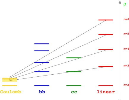
Figure 5: $\rho=(E_{n}-E_{1})/(E_{2}-E_{1})$, where $E_{n}$ is either the $n$th energy level of the physical system or the $n$th eigenvalue of the Schrödinger equation corresponding to the indicated potential.

A lot of work has been done to find the phenomenological form of the static potential (see the report of Gromes, Lucha and Schöberl (1991)). Lowest order perturbation theory for QCD gives a flavour-independent central potential based on the one-gluon exchange, which has a Coulomb-like form (see Exercise 3.1)

$$V_{0}(r)=-{4\over 3}{\alpha_{\rm s}\over r}$$ (7)

where $r$ is the distance between the two quarks and $\alpha_{\rm s}$ is the strong coupling constant . This cannot be the final answer since it does not confine quarks and gives a spectrum incompatible with the data (see Fig. 5). Nevertheless we can regard the one-gluon exchange formula to be valid for $r\simeq 0.1$ fm.

It was found that the addition of some positive power of $r$ to Eq. (7) rescues the phenomenology. The intuitive argument of a constant energy density (string tension), exposed in Sec. 2, led to the flavor-independent Cornell potential (Eichten et al. (1978))

$$V_{0}(r)=-{4\over 3}{\alpha_{\rm s}\over r}+\sigma r+{\rm const.}$$ (8)

Here, $\alpha_{\rm s}$ and $\sigma$ are regarded as free parameters to be fitted on the spectrum. The Schrödinger equation with the potential (8) and parameters $\alpha_{\rm s}=0.39$ and $\sigma=0.182$ GeV² gives quite a satisfactory agreement with the data. In Eichten et al. (1980), the coupling to charmed meson decay-channels was also taken into account. It was found that the mass shifts due to the coupled channel effects are indeed large also below threshold and yet they do not spoil the predictions of the naive potential model. Indeed these effects can essentially be absorbed into a redefinition of the effective parameters.

b

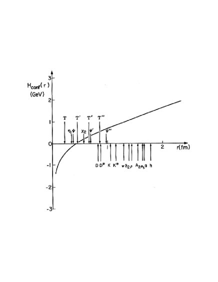
Figure 6: The rms $q\bar{q}$ separations in some representative mesons is shown with respect to the Cornell potential. All the phenomenological potentials agree in the range of $0.1-1$ fm which is the physical range for quarkonia. From Godfrey and Isgur (1985).

Since then several different phenomenological forms of the static potential have been exploited, e.g. the Richardson potential,

$${\displaystyle V_{0}(r)=\int{d^{3}{\bf Q}\over(2\pi)^{3}}\exp{\{i{\bf Q}\cdot{\bf r}\}}{{\rm const.}\over Q^{2}\log(1+Q^{2}/\Lambda^{2})}}$$

(Richardson (1979)), the logarithmic potential, $V_{0}(r)=A\log(r/r_{0})$ (Quigg and Rosner (1977)), the Martin potential, $V_{0}(r)=A(r/r_{0})^{\alpha}$ (Martin (1980)). By fitting the parameters, all these potentials can reproduce the spectrum. This is not surprising if we look at Fig. 6: the potentials essentially agree in the region $r\sim 0.1\div 0.8$ fm in which the $\sqrt{\langle r^{2}\rangle}$ for quarkonia sits (Buchmüller and Tye (1981)). On the other hand, it is a considerable limit of the potential approach that the connection with the true QCD parameters of Eq. (1) remains totally hidden and mysterious.

However, the existence of a spin substructure in the spectrum indicates that relativistic corrections to the static central potential $V_{0}$ have to be taken into account. From the radial level splitting (see Exercise 3.2) as well as from the fits with the phenomenological potential, we find for

$$c\quad{\rm in}\quad\psi, v^{2}\simeq 0.3$$

$$b\quad{\rm in}\quad\Upsilon, v^{2}\simeq 0.1\quad,$$ (9)

and therefore we expect relativistic corrections of order $20\div 30\%$ for the charmonium spectrum and up to $10\%$ for the bottomonium spectrum. This determination of the heavy quark velocity in the bound states is confirmed by lattice calculation, see Tab.1. Notice that relativistic corrections are of critical importance for the observables sensitive to the details of the wave functions (e.g. the radiative transitions ) (Mc Clary et al. (1983)).

$nL$	$\langle{v_{b}^{2}}\rangle$	$\langle{v_{c}^{2}}\rangle$	$\sqrt{\langle{r_{b}^{2}}\rangle}/$fm	$\sqrt{\langle{r_{c}^{2}}\rangle}/$fm
$1S$	0.080	0.27	0.24	0.43
$2S$	0.081	0.35	0.51	0.85
$3S$	0.096	0.44	0.73	1.18
$1P$	0.068	0.29	0.41	0.67
$2P$	0.085	0.39	0.65	1.04
$1D$	0.075	0.34	0.54	0.87

Table 1: From Bali et al. (1997). Notice that for a Coulombic system $v\sim\alpha/n$ and for a confined system $v$ grows with $n$.

The phenomenological potential model predictions of the relativistic corrections are calculated by means of a Breit–Fermi Hamiltonian of the type

$$H=\sum_{j=1,2}\left(m_{j}+{p_{j}^{2}\over 2m_{j}}-{p_{j}^{4}\over 8m_{j}^{3}}\right)+V_{0}+V_{\rm SD}+V_{\rm VD}.$$ (10)

The $1/m^{2}$ spin-dependent $V_{\rm SD}$ and velocity-dependent $V_{\rm VD}$ potentials are derived from the semirelativistic reduction of the Bethe–Salpeter (BS) equation for the quark-antiquark connected amputated Green function or, equivalently at this level, from the semirelativistic reduction of the quark-antiquark scattering amplitude with an effective exchange equal to the BS kernel. Several ambiguities are involved in this procedure, due on one hand to the fact that we do not know the relevant confining Bethe–Salpeter kernel, on the other hand due to the fact that we have to get rid of the temporal (or energy $Q_{0}$, $Q=p_{1}-p_{1}^{\prime}$ being the momentum transfer) dependence of the kernel to recover a potential (instantaneous) description. It turns out that, at the level of the approximation involved, the spin-independent relativistic corrections at the order $1/m^{2}$ depend on the way in which $Q_{0}$ is fixed together with the gauge choice of the kernel. The Lorentz structure of the kernel is also not known.

On a phenomenological basis, the following ansatz for the kernel was intensively studied

$$I(Q^{2})=(2\pi)^{3}\left[\gamma_{1}^{\mu}\gamma_{2}^{\nu}P_{\mu\nu}J_{v}(Q)+J_{s}(Q)\right]$$ (11)

in the instantaneous approximation $Q_{0}=0$. Notice that the effective kernel above was taken with a pure dependence on the momentum transfer $Q$. But, of course, the dependence on the quark and antiquark momenta could have been more complicated. The vector kernel $\gamma_{1}^{\mu}\gamma_{2}^{\nu}P_{\mu\nu}J_{v}(Q)$ corresponds to the one gluon exchange, and e.g. in the Coulomb gauge $P_{\mu\nu}$ has the structure $P_{\mu\nu}=g_{\mu\nu}+\displaystyle{J_{v}^{\prime}(-{\bf Q}^{2})\over J_{v}(-{\bf Q}^{2})}Q_{\mu}Q_{\nu}-\displaystyle{J_{v}^{\prime}(-{\bf Q}^{2})\over J_{v}(-{\bf Q}^{2})}Q_{0}(Q_{\mu}n_{\nu}+Q_{\nu}n_{\mu})$ where the prime indicates the derivative and $n_{\mu}$ is the unit vector in the time direction. The scalar kernel $J_{s}(Q)$ accounts for the nonperturbative interaction. The semirelativistic reduction of the kernel (11) (in the instantaneous approximation, with the Coulomb gauge fixed for the vectorial part, in the centre of mass frame ${\bf p}_{1}=-{\bf p}_{2}={\bf q},{\bf p}^{\prime}_{1}=-{\bf p}^{\prime}_{2}={\bf q}^{\prime},{\bf Q}\equiv{\bf q}-{\bf q}^{\prime}$ and in the equal mass case), gives

$$V_{0} = \tilde{J}_{s}(r)+\tilde{J}_{v}(r)$$ (12)

$$V_{\rm SD} = {3\over m^{2}}{1\over r}\left({d\tilde{J}_{v}\over dr}-{1\over 3}{d\tilde{J}_{s}\over dr}\right){\bf S}\cdot{\bf L}$$

$$+ {1\over m^{2}}\left({1\over r}{d\tilde{J}_{v}\over dr}-{d^{2}\tilde{J}_{v}\over dr^{2}}\right)S_{1}^{h}\left({r^{h}r^{k}\over r^{2}}-{\delta^{hk}\over 3}\right)S^{k}_{2}+{2\over 3m^{2}}\Delta\tilde{J}_{v}(r){\bf S}_{1}\cdot{\bf S}_{2}$$

$$V_{\rm VD} = {1\over 4m^{2}}\Delta(\tilde{J}_{s}+\tilde{J}_{v})-{1\over 4m^{2}}q^{h}\tilde{J}_{s}q^{h}+{1\over 2m^{2}}q^{h}\left(\delta^{hk}-{\partial_{h}\partial_{k}\over\partial^{2}}\tilde{J}_{v}\right)q^{k}$$ (14)

with $\tilde{J}_{v,s}({\bf r})\equiv\displaystyle\int{d^{3}{\bf Q}}\,e^{i{\bf Q}\cdot{\bf r}}J({\bf Q})_{v,s}$. Taking $J_{v}\!=\!\displaystyle-{1\over 2\pi^{2}}{4\over 3}{1\over{\bf Q}^{2}}$ and $J_{s}\!=\!\displaystyle-{\sigma\over\pi^{2}}{1\over{\bf Q}^{4}}$, $V_{0}$ reproduces the Cornell potential.

The confining part of the kernel is usually chosen to be a Lorentz scalar in order to match the data on the fine separation. Indeed, the ratio $\rho_{FS}$ of the fine structure splitting

$$\rho_{FS}={M(^{3}P_{2})-M(^{3}P_{1})\over M(^{3}P_{1})-M(^{3}P_{0})}$$ (15)

is $\rho_{FS}=0.8$ for a pure vector Coulomb exchange while the data give $\rho_{FS}\simeq 0.49,0.66,0.57$ for the $c\bar{c}(1P),b\bar{b}(1P)$ and $b\bar{b}(2P)$ respectively. Adding a scalar exchange gives a contribution to the spin orbit interaction that reduces the vector part and thus also the value of the ratio $\rho_{FS}$ (Schnitzer (1978)). Moreover, since the two terms, vectorial short range and scalar long range exchange, contribute with opposite signs, we expect that at high orbital excitations, where the $Q\bar{Q}$ pair probes large average distances (see Fig. 6), the triplet multiplet inverts with reference to the ordering of the low excitation multiplets (i.e. $M(^{3}L_{L+1})\geq M(^{3}L_{L})\geq M(^{3}L_{L-1})$ at low $L$ and the reverse at high $L$). The fine structure turns out to be a nice test for the form of the confining interaction (cf. e.g. Isgur (1998)).

We have presented a way to obtain phenomenologically the ${1/m^{2}}$ relativistic corrections. However, this is not really rewarding. In a confining interaction the average $\langle p^{2}\rangle$ increases with the excited states (see Tab. 1) and so the pattern of the excited levels is likely to be considerably distorted if the nonperturbative relativistic corrections are not the appropriate ones. Indeed, fits made with only the static potential turn out to be better than fits made with the interaction (12)-(14) (Brambilla et al. (1990)). Moreover, there are characteristics of the spectrum, like the hyperfine separation as well as the leptonic decays, that are due to processes taking place at very short scale. In this case it is important to add higher order perturbative corrections to the one gluon exchange as well as the running of $\alpha_{\rm s}$. In the phenomenological potential framework it is somehow ambiguous how to take into account the running of $\alpha_{\rm s}(\mu)$ as well as the scale $\mu$.

In this section we realized that the description of the heavy meson spectrum turns out to be a priori a quite complicate problem with an interplay of different relevant scales as well as of perturbative and nonperturbative effects. The conclusion is that we badly need, on one hand a framework in which relativistic as well as perturbative corrections to the quark-antiquark interaction can be evaluated unambiguously and systematically and, on the other hand a clear, well founded and eventually computable approach to the long range quark-antiquark interaction which is essentially nonperturbative. We need this both at a concrete level, in order to make quantitative predictions in which the size of the neglected terms can be estimated, and both at a fundamental level, in order to use the spectrum to get some insight into the confinement mechanism.

In the next section we address the problem of how to study quark confinement beyond phenomenological models i.e. in a QCD based framework and we give a criterium that decides whether a gauge theory is confined or not.

3. Exercises

• Consider the quark-antiquark scattering

  $$q_{i}(p_{1},\sigma_{1})+\bar{q}_{j}(p_{2},\sigma_{2})\to q_{k}(q_{1},\tau_{1})+\bar{q}_{l}(q_{2},\tau_{2})$$ (16)

  where $i,j,\cdots=1,2,3$ label the colour indices. Remembering that the quarks in the meson are in a colour-singlet state and introducing the meson colour wavefunctions $\delta_{ij}/\sqrt{3}$, calculate the $T$-matrix element, extract the first contribution in the nonrelativistic limit and obtain, via Fourier transform, the perturbative one gluon exchange potential of Eq. (7). Show that the contribution of the annihilation graph vanishes.

• Consider the average excitation energy in charmonium and bottomonium (e.g. $M_{\Upsilon}^{\prime}-M_{\Upsilon}$). This should be of the order of the average kinetic energy $E\simeq mv^{2}$. Taking $m$ to be roughly half of the ground state mass obtain the estimates (9) for the quark velocities.

• Consider the same scattering of (16) with the exchange given in Eq. (11). Obtain the result (12)-(14) by computing the scattering matrix element of this process, expanding up to the ${1/m^{2}}$ order and Fourier transforming.

• Consider the same scattering matrix of Exs. 3.1 and 3.3 but with a kernel of the type $\displaystyle I=\gamma^{1}_{5}\gamma^{2}_{5}V_{p}(Q)$. Show that there is no static potential in the nonrelativistic limit of the matrix element. Discuss the result in relation to the deuteron.

4 The Wilson Loop: Confinement and Flux Tube Formation

The most powerful technique in order to extract nonperturbative information from QCD is the lattice gauge theory approach. This has been undoubtedly successful and rewarding and has produced over the last years an impressive amount of results. Yet, in spite of almost two decades of intensive efforts the characteristics of QCD associated with colour confinement are still not understood. It is our belief that some insight in the mechanism of confinement cannot be obtained without developing, in strict connection with lattice QCD, also analytic methods. In this way information coming from the lattice can be inserted inside analytic models or vice versa lattice calculations can be used in order to interpret analytic models.

To this aim we need an unambiguous way of establishing a gauge invariant and systematic procedure to calculate the quark dynamics. In Sec. 5, we will show that this is feasible in the case of heavy quarks in which the whole dynamics can be reduced to few expectation values of chromoelectric and chromomagnetic fields that can be calculated analytically (once a model for the QCD vacuum is assumed) or numerically on the lattice. Then, the comparison between the two results supply us with hints about the mechanism of confinement.

The simplest manifestation of confinement in quenched QCD is the linear rising of the potential $V_{0}(r)$ between static colour sources in the fundamental representation. In this section we will show how this has been clearly proved and connected to the formation of a chromoelectric flux tube between the quarks. The question of the nature and the origin of these nonperturbative field configurations will be addressed in Sec. 6.

4.1 The QCD static potential and the Wilson loop

Let us consider a locally gauge invariant quark-antiquark singlet state

$$|\phi_{\alpha\beta}^{lj}\rangle\equiv{\delta_{lj}\over\sqrt{3}}\bar{\psi}^{i}_{\alpha}(x)U^{ik}(x,y,C)\psi^{k}_{\beta}(y)|0\rangle$$ (17)

where $i,j,k,l$ are colour indices (that will be suppressed in the following), $|0\rangle$ denotes the ground state and the Schwinger string line has the form

$$U(x,y;C)=P\exp\left\{ig\int_{y}^{x}A_{\mu}(z)\,dz^{\mu}\right\}\,,$$ (18)

where $A_{\mu}$ is the gauge potential of Eq. (2), $g$ the QCD coupling constant, and the integral is extended along the path $C$. The operator $P$ denotes the path-ordering prescription which is necessary due to the fact that $A_{\mu}$ are non-commuting matrices.

Remembering that under a $SU(3)$ gauge transformation ${\cal V}(\theta)$ $=$ $\exp({-i\theta})$ $\simeq 1-i\theta$, the gauge potential undergoes the transformation $A_{\mu}$ $\to$ $A_{\mu}$ $+$ $i[\theta,A_{\mu}]$ $+$ $g^{-1}\partial_{\mu}\theta$, we obtain the transformation law of the string

$$U^{\prime}(x,y;C)=\exp{\{i\theta(x)}\}U(x,y;C)\exp{\{-i\theta(y)\}}$$ (19)

and then it is clear that (17) is a gauge-invariant state. Actually, it is a colour singlet and we are interested only in colour singlet being the only existing initial and final states.

The quark-antiquark potential can be extracted from the quark-antiquark Green function. A simple example clarifies in which way. Let us consider the following two-particle Green function

$$G(T)=\langle\phi({\bf x},0)|\phi({\bf y},T)\rangle=\langle\phi({\bf x},0)|\exp{(-iHT)}|\phi({\bf y},0)\rangle.$$ (20)

Inserting a complete set of energy eigenstates $\psi_{n}$ with eigenvalues $E_{n}$ and making a Wick rotation we find

$$G(-iT) = \sum_{n}\langle\phi({\bf x},0)|\psi_{n}\rangle\langle\psi_{n}|\phi({\bf y},0)\rangle\exp{(-E_{n}T)}$$ (21)

$$\to \langle\phi({\bf x},0)|\psi_{0}\rangle\langle\psi_{0}|\phi({\bf y},0)\rangle\exp{(-E_{0}T)}\quad{\rm for}\quad T\to\infty$$

which gives the Feynman–Kac formula for the ground state energy

$$E_{0}=-\lim_{T\to\infty}{\log G(-iT)\over T}.$$ (22)

The only condition for the validity of Eq. (22) is that the $\phi$ states have a non-vanishing component over the ground state. The same is still true for finite $T$ if the overlap with the ground state is not too small. This is precisely the way in which hadron masses are computed on the lattice. Of course, many tricks are used in order to maximize the overlap with the ground state in consideration. If the $\phi$ state denotes a state of two exactly static particles interacting at a distance $r$, then the ground state energy is a function of the particle separation, $E_{0}\equiv E_{0}(r)$, and gives the potential of the first adiabatic surface. With this in mind, we will perform in the remaining of this section an explicit evaluation of the quark-antiquark Green function for infinitely heavy quarks ($m_{j}\to\infty$) and for large temporal intervals ($T\to\infty$).

In the following we will be working in the Euclidean space taking advantage of the usual relation between Euclidean position $x^{E}_{\mu}$, momentum $k^{E}_{\mu}$, field $A^{E}_{\mu}$, gamma matrices $\gamma^{E}$ and the corresponding quantities in Minkowski space

$$t^{E}=it^{M}\qquad\quad~{}x_{i}^{E}=x_{i}^{M}$$

$$k_{4}^{E}=-ik_{0}^{M}\qquad\>k_{i}^{E}=k_{i}$$

$$A_{4}^{E}=-iA_{0}^{M}\qquad\!A_{i}^{E}=A_{i}^{M}$$

$$\gamma_{4}^{E}=\gamma_{0}\qquad\qquad\!\gamma_{i}^{E}=-i\gamma^{i}.$$ (23)

Let us assume that at a time $t=0$ a quark and an antiquark are created and that they interact while propagating for a time $t=T$ at which they are annihilated. Then ($x_{j}=({\bf x}_{j},T),y_{j}=({\bf y}_{j},0)$)

$$G_{\beta_{1}\beta_{2}\alpha_{1}\alpha_{2}}(T)$$

$$=\langle 0|\bar{\psi}_{\beta_{2}}({\bf y}_{2},0)U(y_{2},y_{1})\psi_{\beta_{1}}({\bf y}_{1},0)\bar{\psi}_{\alpha_{1}}({\bf x}_{1},T)U(x_{1},x_{2})\psi_{\alpha_{2}}({\bf x}_{2},T)|0\rangle$$

$$={1\over Z}\int{\cal D}\psi{\cal D}\bar{\psi}{\cal D}A\,\bar{\psi}_{\beta_{2}}({\bf y}_{2},0)U(y_{2},y_{1})\psi_{\beta_{1}}({\bf y}_{1},0)$$

$$\qquad\qquad\times\bar{\psi}_{\alpha_{1}}({\bf x}_{1},T)U(x_{1},x_{2})\psi_{\alpha_{2}}({\bf x}_{2},T)e^{-\int L\,\,d^{4}x}$$ (24)

where $L$ is the Euclidean version of Eq. (1), $L=L_{YM}+L_{F}={1\over 4}F_{\mu\nu}F_{\mu\nu}+\bar{\psi}(\gamma_{\mu}D_{\mu}+m)\psi$. The indices $\alpha,\beta$ are spinor indices, while the detailed structure of the colour indices is not displayed. Since the action is quadratic in the quark fields, it is possible to perform the fermion integration

$$G_{\beta_{1}\beta_{2}\alpha_{1}\alpha_{2}}(T)$$

$$={1\over Z}\int{\cal D}A\,\big{(}{\rm Tr}\{S_{\alpha_{2}\beta_{2}}(x_{2},y_{2};A)U(y_{2},y_{1})S_{\beta_{1}\alpha_{1}}(y_{1},x_{1};A)U(x_{1},x_{2})\}$$

$$\qquad-{\rm Tr}\{S_{\beta_{1}\beta_{2}}(y_{1},y_{2};A)U(y_{2},y_{1})\}{\rm Tr}\{S_{\alpha_{2}\alpha_{1}}(x_{2},x_{1};A)U(x_{1},x_{2})\}\big{)}$$

$$\qquad\times\det{K(A)}e^{-\int L_{YM}d^{4}x}$$ (25)

where the trace is over the colour indices and $K$ is the fermionic determinant of the matrix $K_{\alpha x\beta y}(A)\equiv[\gamma_{\mu}D_{\mu}+m]_{\alpha\beta}\delta^{4}(x-y)$. In the following, we will assume the quenched approximation, $\det K=1$. The second term in Eq. (25) describes quark-antiquark annihilation and hence appears only for quarks of the same flavour. Since this effect is dominated by the perturbative two or three gluons exchange in the s channel we will not consider this term any more here. Then we obtain

$$G(T)\simeq{1\over Z}\int{\cal D}A\,{\rm Tr}\{S(x_{2},y_{2};A)U(y_{2},y_{1})S(y_{1},x_{1};A)U(x_{1},x_{2})\}e^{-\int L_{YM}d^{4}x}.$$ (26)

In Eq. (26) $S(x,y;A)$ denotes the quark propagator in the presence of the gluon field $A_{\mu}$. It obeys the equation

$$(\gamma_{\mu}D_{\mu}+m)S(x,y;A)=\delta^{4}(x-y).$$ (27)

This is in principle a system of coupled partial differential equations that cannot be solved in a closed form for an arbitrary $A_{\mu}$. However, we are interested in the limit $m\to\infty$. In this approximation (Wilson (1974), Brown and Weisberger (1979)) we can replace $S$ by the static solution $S_{0}$ obtained dropping the spatial part of the gauge-covariant derivative in (27) while maintaining the time component. This approximation maintains the manifest gauge invariance. Then we have

$$(\gamma_{4}D_{4}+m)S_{0}(x,y;A)=\delta^{4}(x-y)$$ (28)

which is an ordinary differential equation solvable in a closed form. Indeed, we can get rid of the $A_{4}$ in the equation making the ansatz

$$S_{0}(x,y;A)={\rm P}\exp{\left\{ig\int_{x_{4}}^{y_{4}}dtA_{4}({\bf x},t)\right\}}\hat{S}_{0}(x-y)$$ (29)

with $\hat{S}_{0}$ satisfying

$$(\gamma_{4}\partial_{4}+m)\hat{S}(x-y)=\delta^{4}(x-y).$$ (30)

Therefore the solution has the form

$$S_{0}(x,y;A) = \delta^{3}({\bf x}-{\bf y}){\rm P}e^{ig\int_{x_{4}}^{y_{4}}dtA_{4}({\bf x},t)}\left\{\theta(x_{4}-y_{4}){1+\gamma_{4}\over 2}e^{-m(x_{4}-y_{4})}\right.$$ (31)

$$\qquad\qquad\left.+\theta(y_{4}-x_{4}){1-\gamma_{4}\over 2}e^{-m(y_{4}-x_{4})}\right\}.$$

This expression shows that the time evolution of a (infinitely) heavy quark field consists purely in the accumulation of phase determined by $A_{4}$ and the quark mass (cf. Ex. 4.1.1). The spatial delta function says that the infinitely heavy quark cannot propagate in space.

b

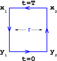
Figure 7: Static Wilson loop with contour $\Gamma_{0}$.

The quark-antiquark Green function is given by

$$G_{\beta_{1}\beta_{2}\alpha_{1}\alpha_{2}}(T) {\buildrel m_{j}\to\infty\over{\longrightarrow}} \,\delta^{3}({\bf x}_{1}-{\bf y}_{1})\delta^{3}({\bf x}_{2}-{\bf y}_{2})(P_{+})_{\beta_{1}\alpha_{1}}(P_{-})_{\alpha_{2}\beta_{2}}$$ (32)

$$\times e^{-(m_{1}+m_{2})T}\langle{\rm Tr}\,{\rm P}e^{ig\oint_{\Gamma_{0}}dz_{\mu}A_{\mu}(z)}\rangle$$

with $P_{\pm}\equiv(1\pm\gamma_{4})/2$. The integral in Eq. (32) extends over the circuit $\Gamma_{0}$ which is a closed rectangular path with spatial and temporal extension $r=|{\bf x}_{1}-{\bf x_{2}}|$ and $T$ respectively, and has been formed by the combination of the path-ordered exponentials along the horizontal (=time fixed) lines, coming from the Schwinger strings, and those along the vertical lines coming from the static propagators (see Fig. 7). The brackets in (32) denote the pure gauge vacuum expectation value. In Euclidean space

$$\langle f[A]\rangle\equiv{1\over Z}\int{\cal D}Af[A]e^{-\int d^{4}xL^{E}_{YM}}.$$ (33)

From Eq. (32) it is clear that the dynamics of the quark-antiquark interaction is contained in

$$W(\Gamma_{0})={\rm Tr\,P}e^{\displaystyle ig\oint_{\Gamma_{0}}dz_{\mu}A_{\mu}(z)}.$$ (34)

This is the famous (static) Wegner–Wilson loop (Wegner (1971) and Wilson (1974)). In the limit of infinite quark mass considered, the kinetic energies of the quarks drop out of the theory, the quark Hamiltonian becomes identical with the potential (see Ex. 4.1.1) while the full Hamiltonian contains also all types of gluonic excitations. According to the Feynman–Kac formula the limit $T\to\infty$ projects out the lowest state i.e. the one with the “glue” in the ground state. This has the role of the quark-antiquark potential for pure mesonic states. Now, comparing Eq. (32) with Eq. (21) and considering that the exponential factor $\exp{(-(m_{1}+m_{2})T)}$ just accounts for the the fact that the energy of the quark-antiquark system includes the rest mass of the pair, we obtain

$$V_{0}(r)\equiv E(r)=-\lim_{T\to\infty}{1\over T}\log\langle W(\Gamma_{0})\rangle.$$ (35)

The quark degrees of freedom have now completely disappeared and the expectation value in (35) has to be evaluated in the pure Yang–Mills theory ((Wilson (1974), Brown and Weisberger (1979)). Notice that the potential is given purely in terms of a gauge invariant quantity (the Wilson loop precisely). In this way we have reduced the calculation of the static potential to a well posed problem in field theory: to obtain the actual form of $V_{0}$ we need to calculate the QCD expectation value of the static Wilson loop.

We conclude this section pointing out that Eq. (35) is rigorously true for static sources. For (realistic) heavy quarks with finite mass, the static potential, interpreted as the static limit of the potential appearing in the Schrödinger equation, could in principle not coincide exactly with Eq. (35). Actually it does not. The reason is that in QCD quarks in the static limit can still change colour by emission of gluons. This introduces a new dynamical scale in the evaluation of the potential from Eq. (35) of the order of the kinetic energy which is finite if the quarks have finite mass. In perturbative QCD this new scale is given by the difference between the singlet and the octet potential. Contributions of the same order of the kinetic energy are not of potential type and have to be explicitly subtracted out from Eq. (35). In the next section we will give the leading effect of this subtraction on the static Wilson loop. For an extended analysis we refer to Brambilla et al. (1999).

4.1 Exercises

• Consider a particle of mass $m$ moving in a potential $V(x)$ in one space dimension. The propagator is given by $\displaystyle K(x^{\prime},t;x,0)=\langle x^{\prime}|\exp{(-iHt)}|x\rangle$ with $H=\displaystyle{p^{2}\over 2m}+V(x)$. Obtain the form of the propagator $K$ in the static limit $m\to\infty$ and compare it with Eq. (31).

• Consider quenched QED. Show that the functional generator for the QED Lagrangian with a source term added of the form $J_{\mu}(x)A_{\mu}(x)$ with $J_{\mu}(x)=e\delta_{\mu 4}(\delta^{3}({\bf x}-{\bf x}_{1})-\delta^{3}({\bf x}-{\bf x}_{2}))$, coincides with the vacuum expectation value of the static Wilson loop in the limit of infinite interaction time.

4.2 The Wilson loop in perturbative QCD

The Wegner–Wilson loop of contour $\Gamma$ is defined in QCD as

$$W(\Gamma)\equiv{\rm Tr\,P}\,e^{ig\displaystyle\oint_{\Gamma}dz_{\mu}A_{\mu}(z)}.$$ (36)

Due to the presence of the colour trace, it is a manifestly gauge invariant object. The field $A_{\mu}$ can be taken in any representation of $SU(3)$. When describing the quark-antiquark interaction, as in the present case, $A_{\mu}\equiv A_{\mu}^{a}\lambda^{a}/2$. The Wilson loop is called static when the integral is extended to a rectangular $\Gamma_{0}$ as in Fig. 7. Physically, in the static Wilson loop only the time component $A_{4}$ is relevant.

We know from the previous section that the vacuum expectation value of $W$ on the QCD measure gives the static potential. However, we are in trouble when we step in to calculate it. Indeed, if we want to describe the long range quark-antiquark interaction, we should be able to calculate the Wilson loop in the region in which the running coupling constant is no longer small and we should be able to sum up all the relevant diagrams. Unfortunately, we have no methods at hand to sum up such contributions. Worse enough, also usual semiclassical approaches are not doomed to work in this case. We do not know of any dominant and confining configurations in the QCD measure and in the path integral that can make the work! Hence, to obtain information on the behaviour of the Wilson loop in the nonperturbative region we have to resort either to strong coupling expansion and to lattice simulations, see Sec. 4.3 and Sec. 4.5, or to analytic models of the QCD vacuum, see Sec. 6.

However, in the weak coupling region the Wilson loop can be calculated perturbatively. Recently, the fully analytic calculation of the two-loop diagrams contributing to the static potential has been performed (Peter (1997), Schröder (1999)). We refer to the original papers for the details of the calculation. However, due to the high interest, we report here the final result ($\alpha_{\rm s}$ is in the $\overline{MS}$ scheme):

$$V_{0}(r)=-C_{F}{\alpha_{V}(r)\over r}$$ (37)

$$\alpha_{V}(r)=\alpha_{\rm s}(r)\left\{1+\left(a_{1}+{\gamma_{E}\beta_{0}\over 2}\right){\alpha_{\rm s}(r)\over\pi}\right.$$

$$+\left.\left[\gamma_{E}\left(a_{1}\beta_{0}+{\beta_{1}\over 8}\right)+\left({\pi^{2}\over 12}+\gamma_{E}^{2}\right){\beta_{0}^{2}\over 4}+b_{1}\right]{\alpha_{\rm s}^{2}(r)\over\pi^{2}}\right\},$$

where $\gamma_{E}$ is the Euler constant, $a_{0}=1$,

$$a_{1}=\frac{31}{9}C_{A}-\frac{20}{9}T_{F}N_{f}$$

and

$$a_{2} = \Big{(}\frac{4343}{162}+4\pi^{2}-\frac{\pi^{4}}{4}+\frac{22}{3}\zeta_{3}\Big{)}C_{A}^{2}-\Big{(}\frac{1798}{81}+\frac{56}{3}\zeta_{3}\Big{)}C_{A}T_{F}N_{f}$$

$$-\Big{(}\frac{55}{3}-16\zeta_{3}\Big{)}C_{F}T_{F}N_{f}+\Big{(}\frac{20}{9}T_{F}N_{f}\Big{)}^{2}.$$

$C_{F}=4/3$ and $C_{A}=3$ are the Casimir of the fundamental and of the adjoint representation respectively. Moreover in QCD we have $T_{F}=1/2$.

From this result we learn that: the two-loop contribution is nearly as large as the one-loop term, both make the potential more attractive and eventually the perturbative potential seems to be reliable up to a distance $r\Lambda_{QCD}<0.07$, which is considerably smaller than the average radius in quarkonia (see Fig. 6). For larger values a strong scale-dependence remains and the perturbation series breaks down above 0.1 fm. Hence, even the pure perturbative calculation indicates the need of a different long range approach.

We mention that the next perturbative correction to the static potential can be obtained only in an effective theory framework (pNRQCD, see Sec. 5). In that framework the leading log three-loop term has been very recently calculated in Brambilla et al. (1999). It amounts to a correction $C_{A}^{3}\alpha_{\rm s}^{4}(r)/12\pi\log{r\mu^{\prime}}$ to $\alpha_{V}$ in Eq. (37), $\mu^{\prime}$ being the scale of the matching. Notice that the potential comes to depend on the infrared scale $\mu^{\prime}$. This signals the appearance at three-loop of a nonpotential type of contribution to the static Wilson loop which has been subtracted out explicitly at $\mu^{\prime}$.

In QED in the quenched approximation (i.e. neglecting light fermions) the (non-static) Wilson loop can be calculated analytically in a closed form. We sketch here the derivation. We have (in Euclidean space)

$$\langle W(\Gamma)\rangle={\displaystyle\int{\cal D}A\,e^{\displaystyle{1\over 2}\displaystyle\int d^{4}xA_{\mu}\,M_{\mu\nu}A_{\nu}+ie\oint dz_{\mu}A_{\mu}}\over\displaystyle\int{\cal D}A\,e^{\displaystyle{1\over 2}\displaystyle\int d^{4}xA_{\mu}\,M_{\mu\nu}A_{\nu}}}$$ (38)

where $M_{\mu\nu}\equiv\delta_{\mu\nu}\partial^{2}-\partial_{\mu}\partial_{\nu}$ has been obtained by integrating by parts the original QED action. The integral over the $A$ field in Eq. (38) is Gaussian and therefore can be performed provided that a gauge condition is imposed. However, since the Wilson loop is a gauge-invariant quantity, the choice of the gauge is immaterial. We obtain

$$\langle W(\Gamma)\rangle=\exp\left\{{e^{2}\over 2}\oint_{\Gamma}dx_{\mu}\oint_{\Gamma}dx^{\prime}_{\nu}D_{\mu\nu}(x-x^{\prime})\right\}$$ (39)

where $D_{\mu\nu}(x-x^{\prime})\equiv\langle A_{\mu}(x)A_{\nu}(x^{\prime})\rangle$ is the photon propagator. E.g. in Feynman gauge we have $D_{\mu\nu}(x)=-\displaystyle{\delta_{\mu\nu}\over 4\pi^{2}}{1\over x^{2}}$. On a rectangular Wilson loop Eq. (39) becomes

$$\langle W(\Gamma_{0})\rangle=\exp\left\{{e^{2}\over 4\pi r}Tf(r,T)\right\}$$ (40)

with $f(T,r)=\displaystyle{2\over\pi}\left[{\rm arctan}{T\over r}-{r\over 2T}\log(1+{T^{2}\over r^{2}})\right]$, $f\to 1$ for $T\to\infty$ getting back the Coulomb potential.

b

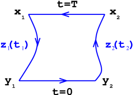
Figure 8: Generalized Wilson loop with contour $\Gamma$.

In the weak coupling region the vacuum expectation value of the (non-static) Wilson loop in QCD can be obtained by making a Gaussian approximation on the functional integral (i.e. by neglecting non-Abelian contributions). In this case, since the contribution coming from the Schwinger strings vanish in the limit $T\to\infty$ and taking advantage of the notation given in Fig. 8, we have

$$\langle W(\Gamma)\rangle\! = \!e^{\displaystyle{4\over 3}g^{2}\displaystyle\oint_{\Gamma}dz^{1}_{\mu}\oint_{\Gamma}dz^{2}_{\nu}D_{\mu\nu}(z_{1}-z_{2})}$$ (41)

$${\buildrel{T\to\infty}\over{\longrightarrow}} \!e^{\displaystyle{4\over 3}g^{2}\displaystyle\int_{t_{i}}^{t_{f}}dt_{1}\int_{t_{i}}^{t_{f}}dt_{2}\dot{z}_{\mu}^{1}(t_{1})\dot{z}_{\nu}^{2}(t_{2})D_{\mu\nu}(z_{1}(t_{1})-z_{2}(t_{2}))}\,,$$

$D_{\mu\nu}$ being the gluon propagator.

4.2. Exercises

• From Eqs. (35) and (41) obtain the QCD one gluon exchange contribution to the static QCD potential.

• Calculate Eq. (40) from Eq. (39).

• From the correspondent of Eq. (75) (Sec. 5) in Euclidean space, obtain the QCD $V_{0}$ and $V_{\rm VD}$ potentials using the weak coupling behaviour of the Wilson loop given in (41) with the gluon propagator first in the Coulomb gauge and then in the Feynman gauge. Demonstrate that, due to the gauge invariance of the Wilson loop, the two expression coincide. [Hint: perform the change of variables $t=(t_{1}+t_{2})/2;\tau=t_{1}-t_{2}$ in the integrals in (41), expand ${\bf z}_{j}$ around $t$ and integrate over $\tau^{+\infty}_{-\infty}$.]

4.3 Lattice formulation, strong coupling expansion and area law

Equation (35) is particularly useful on the lattice where the dynamical variables are unitary matrices associated with the links. We do not want to give here an introduction to lattice QCD (for this we refer the reader to Rothe (1992) and Montvay and Munster (1994)). However, in order to illustrate some interesting results, we recall the basic definitions and concepts.

b

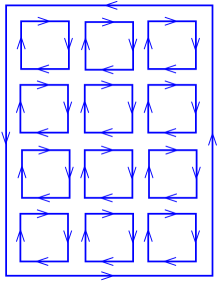
Figure 9: Elementary plaquette on the lattice and tiling of the Wilson loop in strong coupling.

Let us consider QCD in the pure gauge sector on a four-dimensional Euclidean discretized space-time, the “lattice” of step $a$. Lattice sites are denoted by $n$ and lattice directions are denoted by $\mu,\nu$. We define the group element associated with a link, from the lattice site $n$ to $n+\hat{\mu}$ ($\hat{\mu}$ being a unit vector along the axis $\mu$) as

$$U_{\mu}(n)\equiv U(n,n+\hat{\mu})\simeq e^{igaA_{\mu}(n+{\hat{\mu}\over 2})}\quad\quad U^{\dagger}_{\mu}(n)\equiv U(n+\hat{\mu},n).$$ (42)

These are the dynamical variables, the gluonic colour fields that relate the colour coordinate system at different space-time points. From (42) we see that they are represented as a $3\times 3$ colour matrix that can be interpreted as the path-ordered exponential of the continuum colour fields $A_{\mu}(x)$. The gauge transformation on the lattice, ${\cal V}(x_{n})$, acts directly on the link elements

$$U_{\mu}(n)\to{\cal V}^{\dagger}(n+\hat{\mu})U_{\mu}(n){\cal V}(n).$$ (43)

The Yang–Mills action is

$$S=-{\beta\over 3}\sum_{\mu>\nu}\sum_{n}\,{\rm Re}\,{\rm Tr}\,U_{\mu\nu}$$ (44)

with $\beta=6/g^{2}$. The elementary plaquette is the trace of the path-ordered product of links around a unit square (see Fig. 9)

$$U_{\mu\nu}(n)\equiv U_{\mu}(n)U_{\nu}(n+\hat{\mu})U^{\dagger}_{\mu}(n+\hat{\nu})U^{\dagger}_{\nu}(n);\quad\quad U_{P}\equiv{1\over 3}{\rm Re}\,{\rm Tr}\,U_{\mu\nu}.$$ (45)

In the continuum limit ($a\to 0$) expression (44) reduces to the usual Yang–Mills action. The corresponding partition function is

$$Z=\int\prod_{n,\mu}{\cal D}Ue^{-{\beta}\sum_{P}U_{P}}$$ (46)

where the integral is over the group manifold of colour $SU(3)$ for each link matrix $U$.

The Wilson loop is simply the trace of the product of the matrices $U(n,\mu)$ along the contour $\Gamma$ which here is a rectangle. Then

$$\langle W(\Gamma)\rangle=\langle{\rm Tr}\,\prod_{l\in\Gamma}U(l,\mu_{l})\rangle={1\over Z}\int\prod_{n,\mu}DU(n,n+\hat{\mu}){\rm Tr}\,\prod_{l\in\Gamma}U(l,\mu_{l})e^{-{\beta}\sum_{P}U_{P}}.$$ (47)

Of particular interest is the strong coupling expansion on the lattice, which means to expand for large $g$ (small $\beta$). This bears a relation to the string picture that, as we explained, characterizes the long range quark-antiquark interaction. In the strong coupling, we can expand the exponential of the action in (47)

$$\langle W(\Gamma)\rangle={1\over Z}\int\prod_{n,\mu}DU(n,n+\hat{\mu}){\rm Tr}\,\prod_{l\in\Gamma}U(l,\mu_{l})$$

$$\quad\times\left[1-{\beta}\sum_{P}{\rm Tr}\,U_{P}+{1\over 2}{\beta}^{2}\sum_{P}\sum_{P^{\prime}}{\rm Tr}\,U_{P}\,{\rm Tr}\,U_{P^{\prime}}+\cdots\right].$$ (48)

Since each plaquette in the expansion costs a factor $\beta$, the leading contribution in the limit $\beta\to 0$ is obtained by paving the inside of the Wilson loop with the smallest number of elementary plaquettes yielding a non-vanishing value for the integral. Using the orthogonality relations supplied in Exercise 4.3.1, it is possible to show that the relevant configuration is the one presented in Fig. 9 and that

$$\langle W(\Gamma)\rangle\simeq\left({1\over g^{2}}\right)^{N_{P}}\,,$$ (49)

$N_{P}$ being the minimal number of plaquettes required to cover the area enclosed by the path $\Gamma$ (for more details see Creutz (1983)). This corresponds to the area law (Wilson (1974)) since the area enclosed by the path $\Gamma$ is given by $A(\Gamma)=a^{2}N_{P}$. Furthermore, it is possible to demonstrate that the strong coupling expansion (48) has a finite radius of convergence. Hence, for $g^{2}$ large enough, the vacuum expectation value of the Wilson loop has the behaviour

$$\langle W(\Gamma)\rangle\simeq(g^{2})^{-A(\Gamma)/a^{2}}=e^{-\displaystyle{r\,T\log g^{2}\over a^{2}}}$$ (50)

where the last equality holds for a rectangular path $r\times T$. The behaviour of the Wilson loop given by Eq. (50) leads to a linear static potential with

$$\sigma\simeq{\log g^{2}\over a^{2}}.$$ (51)

The layer of plaquettes giving this area contribution corresponds to a constant (chromo)electric field along the string connecting the quark and the antiquark. This suggests once again the relevance of a flux tube description of the nonperturbative interaction and is at the origin of the formulation of the flux tube model of Isgur et al. (1983).

However, we have to keep in mind that the continuum limit of lattice QCD is reached in the weak coupling limit, $\beta\to\infty$. Therefore it is impossible to extrapolate the strong coupling results directly to the continuum physics. Still, we can argue that a rather coarse lattice with large lattice spacing should already give some indicative results for a theory without phase transition. To such a lattice corresponds a large bare coupling $g$ and hence the strong coupling result (50) should give the correct qualitative picture. Our philosophy is to take the behaviour (50) as a reliable suggestion to be used in the continuum physics.

The leading order strong coupling expansion of the Wilson loop in QED is identical to Eq. (50) and therefore produces a linear potential too. However, in the case of QED on the lattice a phase transition is clearly seen (Kogut et al. (1981)) when going from strong coupling to weak coupling. In QCD the analytic proof that there cannot be such a phase transition together with the finite radius of convergence of the strong coupling expansion would be equivalent to a proof of confinement. Such a proof does not exist up to now. However, the numerical lattice simulations present no hint of such a transition in the intermediate coupling region. On the contrary, the strong coupled behaviour $g^{2}(a)\sim e^{\sigma a^{2}}$ continuously goes into the weak coupling $g^{2}(a)\sim 1/\log{a^{-1}}$ as $a\to 0$. Moreover, within the coupling regions accessible to present day computers, there are already overlaps between lattice results and weak coupling expansion, the most impressive being the result of the alpha collaboration, see Capitani et al. (1998).

These results hint to the fact that QCD possesses both the property of asymptotic freedom and colour confinement. In other words the Wilson loop in QCD displays a perimeter law in weak coupling and an area law in strong coupling.

4.3 Exercises

• The orthogonality properties of the group integral in $SU(3)$ are given by

  $$\int dU(n,n+\hat{\mu})[U(n,n+\hat{\mu})]_{ij}=0$$

  $$\int dU(n,n+\hat{\mu})[U(n,n+\hat{\mu})]_{ij}[U^{\dagger}(n,n+\hat{\mu})]_{kl}={1\over 3}\delta_{il}\delta_{jk}$$

  $$\int dU(n,n+\hat{\mu})[U(n,n+\hat{\mu})]_{ij}[U(n,n+\hat{\mu})]_{kl}=0$$

  Using these relations justify the result (49).

4.4 Area law as a criterium for confinement,
duality and the Wilson loop as an order parameter

To see whether QCD shows confinement, one can study the energy of a system composed of a quark and an antiquark along the lines exposed in Sec. 4.1. Then Eq. (35) tells us that it is the Wilson loop and its behaviour that determines the confinement property of the theory. In the previous section we have seen that in QCD in strong coupling expansion the Wilson loop in the fundamental representation obeys an area law behaviour and this in turn via Eq. (35) confirms the property of quark confinement.

For very large loops $\log\langle W(\Gamma)\rangle$ generally exhibits these two types of behaviour: it decreases either as the perimeter or as the area of $\Gamma$. In the first case, expansive loops are allowed and quark and antiquark can be far apart from each other. In the second case quark and antiquark propagate as a bound state. This is the Wilson criterion for confinement of electric charges (Wilson (1974))

$$\langle W(\Gamma)\rangle \sim e^{-KL(\Gamma)}\quad\quad~{}{\rm no}\>{\rm confinement}$$ (52)

$$\langle W(\Gamma)\rangle \sim e^{-K^{\prime}A(\Gamma)}\quad\quad{\rm confinement}$$ (53)

with $L(\Gamma)$ the perimeter of $\Gamma$, $A(\Gamma)$ the minimal area enclosed by $\Gamma$, and $K$ and $K^{\prime}$ dimensionful constants. These are statements about the response of the pure gauge vacuum to external perturbations.

This criterion inspires physical pictures of the QCD vacuum (see Sec. 6). In particular it was suggested by ’t Hooft (see e.g. ’t Hooft (1994)) that a pure non-Abelian gauge theory could display quite a complicate pattern of vacuum phases: 1) The Higgs mode. Only colour magnetic charges are confined. 2) The Coulomb mode, featuring ordinary massless “photons” and no superconductivity or confinement. 3) The confinement mode or “magnetic superconductor”. Quarks (i.e. electric charges) are permanently confined. The properties of these phases are then expressed in terms of operators that create vortices of electric flux (Wilson loops $W_{A}(\Gamma)$, evaluated on the gauge fields $A_{\mu}$) and operators that create vortices of magnetic flux (’t Hooft operators $W_{C}(\Gamma)$, evaluated on the dual potentials $C_{\mu}$). Using the definition of $W_{C}(\Gamma)$ via its commutation relation with $W_{A}(\Gamma)$, ’t Hooft (1979) showed that if $W_{A}(\Gamma)$ obeys an area law, then $W_{C}(\Gamma)$ necessarily satisfies a perimeter law. The phase in which the ’t Hooft operator obeys an area law is the Higgs phase, while that one in which the Wilson loop obeys an area law is the confinement phase. ’t Hooft result is a precise way of saying that the vacuum of a confining theory has the properties of a magnetic superconductor. The key ideas are the fact that a non-Abelian gauge theory can be viewed as an Abelian gauge theory enriched with Dirac magnetic monopoles and the concept of electric-magnetic duality. For QCD this implies that the vacuum behaves as a dual superconductor and confinement is explained through the monopole condensation, see Sec. 6. However, if in an Abelian theory it is possible to introduce dual field strengths and electric potentials $C^{\mu}$ dual to the ordinary (magnetic) potentials $A^{\mu}$ in a straightforward manner, in a non-Abelian theory it is not possible to express the dual potentials explicitly in terms of ordinary potentials. The explicit form of the exact Yang–Mills Lagrangian as a function of the $C^{a}_{\mu}$ fields is unknown. The construction of the long distance limit of the Lagrangian is based on the fact that the dual potentials are weakly coupled since the dual Wilson loop obeys a perimeter law. The quadratic part of the dual Lagrangian is thereby determined. The minimal extension can be constructed under requisite of dual gauge invariance. For a concrete construction of a QCD dual Lagrangian see Baker et al. (1985)-(1995); Maedan et al. (1989) and Sec. 6.

These ideas have originated a quite intensive research activity in the “nonperturbative” physics community in the last few years (in QCD mainly on the lattice while in supersymmetric field theories very promising analytic results are obtained just now, see e.g. Alvarez-Gaumé et al. (1997)). We will come back to this point in Sec. 6.2. Here we refer the reader to the historical papers of Nambu (1974), Mandelstam (1979) and ’t Hooft (1982) and references therein.

4.5 Lattice simulations and lattice results

With the action of Eq. (44), using periodic boundary conditions in space and time and taking a lattice of finite volume and finite spacing, the system has a finite number of degrees of freedom: the gluon fields on the link and (if we add them) the quark fields at the lattice sites. The functional integral over the gauge fields is converted to a multiple integral with a positive definite integrand (in Euclidean space): Eq. (46). Unlike in continuum perturbation theory the calculation of averaged values of gauge invariant observables is done without any gauge-fixing.

For a lattice of $L^{4}$ sites with colour group $SU(3)$ the integral in (46) would be a $8\times 4\times L^{4}$ dimensional integral: the standard approach is to use a Monte Carlo approximation to the integrand. Precisely, a stochastic estimate of the integral is made from a finite number of samples (the “configurations”) of equal weight. For more details see Rothe (1992). Here we are interested only in explaining that in this way we have at our disposal a set of samples of the vacuum, then, it is possible to evaluate the average of fields over these samples and obtain a nonperturbative evaluation of Green functions as well as of any field vacuum correlator.

In this section we present some lattice results on the calculation of the Wilson loop expectation value, the static potential, the flux tube configuration and the determination of the string tension $\sigma$. However, before, we comment briefly on the validity of the lattice results and give few concepts to enable the “reading” of those results.

The lattice is not the real world so that before extracting the physics we have to be sure that: 1) the Green functions have been extracted without contamination (the ground state mass should not be contaminated by pieces coming from the excited states); 2) the lattice size is big enough, we mean that the relevant physical distance should fit in! (finite size error); 3) the statistical errors of the calculation is under control (statistical error); 4) the lattice spacing is small enough, since we have to approach the continuum limit (discretization error). On the other hand the lattice spacing supplies an explicit ultraviolet cut-off.

The last condition is the most subtle one. Let us just sketch the idea. In order to extract the continuum limit from the lattice, it has to be shown that the results do not change if the lattice spacing is decreased further. However, the lattice spacing in physical units is not known directly. Actually it is measured. The lattice simulations are performed at a fixed value of $\beta$ (cf. Eq. (44)). We recall that $\beta=6/g^{2}$ and therefore a large $\beta$ corresponds to a small $g^{2}$. Ensembles at different values of $a$ are obtained by using different bare coupling constants $g$ in the action. However, the value of $a$ for a given value of $g$ is not known a priori but has to be obtained calculating a dimensionful parameter and comparing it to an experiment.

As an example let us consider the string tension $\sigma$. Measured in lattice units it is only a function of the bare coupling: $\hat{\sigma}(g)$, the $\hat{}$ denoting a dimensionless quantity. In physical units, however, it has the dimension of a (mass)², so that the physical string tension is given by

$$\sigma=\lim_{a\to 0}{1\over a^{2}}\hat{\sigma}(g(a)).$$ (54)

It approaches a finite limit for $a\to 0$, if $g$ is tuned with $a$ in an appropriate way. By requiring that in this limit

$$a{\partial\over\partial a}\sigma=0$$ (55)

we obtain

$$\sqrt{\sigma} = c_{\sigma}\Lambda_{L}$$

$$\Lambda_{L} = a^{-1}e^{-1\over 2\beta_{0}g^{2}}(\beta_{0}g^{2})^{-\beta_{1}\over 2\beta_{0}^{2}}(1+O(g^{2}))$$ (56)

where we have used the usual lattice convention for the beta function: $\beta(g)$ $=$ $-\beta_{0}g^{3}$ $-\beta_{1}g^{5}$ $+O(g^{7})$ (which differs for a factor $1/(4\pi)^{2}$ from Eq. (3)) and $\Lambda_{L}$ is independent of $a$ and fixes the mass scale of the theory. This equation tells us again that a perturbative calculation of $\sigma$ is a priori impossible due to the non-analytic behaviour in $g$ of Eq. (56). It is possible to show that all dimensionful physical quantities can be expressed in the form

$$\theta_{phys}=\lim_{a\to 0}{1\over a^{d_{\theta}}}\hat{\theta}(g(a),a)=c_{\theta}(\Lambda_{L})^{d_{\theta}}$$ (57)

$d_{\theta}$ being the naive dimension. Then, for small lattice spacing we can determine the universal function $g=g(a)$ by fixing the l.h.s. of (56) at the physical value of the string tension. This gives $g$ as a function of $a\sqrt{\sigma}$

$$g^{2}(a)=-{1\over 2\beta_{0}\log(a\Lambda_{L})}$$ (58)

(where $\Lambda_{L}$ is now determined by the physical condition imposed) which ensures the finiteness of any observable and allows us to convert them to physical units.

The continuum limit has to be taken at a constant physical volume $L^{4}$. As $a$ is decreased the number of lattice points $\hat{L}={L/a}$ increases. Therefore, a finite computer limits the lattice spacing to $a\geq a_{\rm min}>0$. In practice one is looking for scaling of the results within this window or at least checking that the results follow the expected leading order $a$ dependence in order to safely extrapolate them to $a=0$. A typical value for lattice simulations of QCD is $\beta\simeq 6$ and hence the bare coupling constant is $\alpha_{\rm s}=g^{2}/(4\pi)\simeq 0.08$. In the early years of lattice QCD it was widely assumed that at least for $\beta\simeq 6$, two-loop perturbation theory can be applied to $a(g)$. Therefore, after having determined $a$ at a coupling $g$, the $\Lambda$ parameter was extracted and $a(g\prime)$ for $g\prime\neq g$ computed via perturbation theory. Nowadays, the lattice spacing is determined separately for each simulation point $\beta$ by inputting one experimental value. In doing so, $a(g)$ is obtained as a function of the bare lattice $g$. One finds big deviations from perturbation theory (asymptotic scaling) that are related to the importance of the so called tadpole diagrams in lattice perturbation theory (see e.g. Michael (1997), Davies (1997) and Lepage et al. (1993) for these developments).

The actual methods of simulating lattice QCD and extracting physical information have reached quite a high level of sophistication and we refer the interested reader to the reviews (e.g. Rothe (1992), Davies (1997), Montvay and Munster (1994)). The above discussion should be sufficient to make clear that: 1) lattice simulations are performed at a fixed value of $\beta$, 2) the value of $\beta$ is connected with the lattice spacing $a$, 3) results relevant for continuum physics are effectively independent of $a$ (scaling) 4) the extraction of the physical results requires to fix $a$ and in the quenched approximation it may be dependent on the experimental quantity chosen to fix it. It is, therefore, important to know what quantity was chosen when looking at the lattice data.

b

Figure 10: Static potential at $\beta=6.0$ and $\beta=6.2$ in the quenched approximation. The solid line is a fit of the form of Eq. (61). Bali et al. (1997).

Now let us come to some results. First, we discuss the lattice measure of $\sigma$. The lattice counterpart of Eq. (35) is

$$\hat{V}(\hat{r})=-\lim_{\hat{T}\to\infty}{1\over\hat{T}}\log W(\hat{r},\hat{T})$$ (59)

where $W(\hat{r},\hat{T})$ denotes the expectation value of a Wilson loop with spatial and temporal extension $\hat{r}$ and $\hat{T}$ respectively. Assuming that $W(\hat{r},\hat{T})=\exp\{\hat{\sigma}\hat{r}\hat{T}-\hat{\delta}(\hat{r}+\hat{T})+\hat{\gamma}\}$, the famous Creutz ratio

$$\chi(\hat{r},\hat{T})=-\log\left({W(\hat{r},\hat{T})W({\hat{r}}-1,{\hat{T}}-1)\over W(\hat{r},{\hat{T}}-1)W({\hat{r}}-1,\hat{T})}\right)$$ (60)

coincides with the string tension, since the parameters $\hat{\delta}$ and $\hat{\gamma}$ drop out. The original calculation (Creutz et al. (1982)) was performed on a $6^{4}$ lattice and the asymptotic scaling seemed to show up for values of $\beta$ slightly below 6.0. This measurement of a string tension different from zero from the strong coupling region to the asymptotic scale region, without any indication of a phase transition in the intermediate region, constituted the first evidence of quark confinement in QCD.

In Fig. 10 we show the most recent lattice measurement of the quenched static potential from Eq. (59) on a hypercubic lattice $V=16^{4}$ at $\beta=6.0$ and $V=32^{4}$ at $\beta=6.2$. These values correspond to inverse lattice spacings $a^{-1}\simeq 2.1$ GeV and $a^{-1}\simeq 2.9$ GeV respectively. The scale is adjusted to optimally reproduce the bottomonium level splittings (Bali et al. (1997)). The fit curve corresponds to the parameterization

$$V_{0}(r)=-{e\over r}+\sigma r+{f\over r^{2}}$$ (61)

which clearly confirms the Cornell potential (8) (the $1/r^{2}$ correction, that accounts for the running of the coupling, is not meant to be physical but has been introduced to effectively parameterize the data within the given range of $r$). The parameters take the value: $e=0.321$ and $\sigma=(468$ MeV$)^{2}$. The coefficient of the Coulomb term is quite far from the effective value for $\alpha_{\rm s}$ coming from the potential models. Notice that the lattice potential becomes clearly linear around $0.2$ fm. Similar lattice measurements exist for the unquenched static potential (see e.g. Bali (1998)): the string is found to break down around a quark-antiquark distance of about 1.2 fm.

The static potential in Fig. 10 has been extracted as the ground state energy of the quark-antiquark configuration (cf. Eq. (22)), which in turn corresponds to the lowest energy configuration of the “glue” between the quarks. Yet, also the excited gluonic modes have been measured on the lattice and the corresponding potentials have been adiabatically extracted. This should corresponds to the potential of heavy hybrids. For further details of this confirmation of the excited structure of the flux tube we refer the reader to Michael (1997), Morningstar et al. (1998).

b

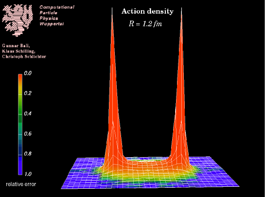
Figure 11: Action density distribution between two static quarks in $SU(2)$ measured on a lattice $V=32^{4}$ at $\beta=2.5$. The physical quark-antiquark distance is 1.2 fm. Bali et al. (1995).

Lattice studies have been undertaken to probe the energy momentum tensor of the colour fields. The probe used is the gauge-invariant insertion of a plaquette in the presence of a static Wilson loop. Depending on the Lorentz orientation of the plaquette, this corresponds to the average of a (chromo)electric or a (chromo)magnetic field in the presence of quark sources. Lattice sum rules can be used to normalize these distributions and to relate them to the $\beta$ function. For separations $r>0.7$ fm, a string-like spatial distribution is found with a transverse rms width increasing very slowly with $r$ and reaching a rather constant value between 1 and 2 fm. The physical value for this constant ranges between 0.5 and 0.75 fm. The averages of the squared components of the colour fields (which are gauge invariant quantities) are found to be roughly equal (i.e. $\langle E^{2}_{i}\rangle\sim\langle B^{2}_{j}\rangle$ in the presence of the Wilson loop, for $i,j=1,2,3$). This implies that the energy density is much smaller than the action density (in Euclidean space). (See Sec. 6.3 for a discussion.) The result for the action density is presented in Fig. 11 and is quite impressive! The formation of the interquark flux tube is evident. The interpretation of this phenomenon is the following. When the distance between the quarks becomes larger than some critical value (connected to $\Lambda_{QCD}$) the branching of the gluons, due to the non-Abelian nature of QCD, becomes so intensive that it makes no sense to speak about individual gluons. A coherent effect develops with the subsequent formation of the flux tube. It is conjectured that a specific organization of the QCD vacuum makes this kind of configuration energetically favorable (see Sec. 6).

However, lattice QCD seems more suitable to ask “what” and not “why”. Here, we have shown some model independent results on the quark interaction that provide evidence of quark confinement but do not explain why quarks are confined. Eventually, to get some insight in the quark confinement mechanism, it is necessary to build up and use some analytic models. The role of the lattice measurements will then be to validate these models. The combination of analytic and lattice techniques will give us some information on the nature of the nonperturbative quark interaction.

Finally, we mention that there are a lot of measurements of hadron masses performed in lattice QCD as well as in lattice nonrelativistic QCD (NRQCD). However, since in these lectures we are more interested in the mechanism of confinement as well as in developing analytic approaches to it, we refer the reader to the literature (see e.g. Davies (1997)).

5 The Heavy Quark Interaction

In this part of the lectures we summarize some nonperturbative analytic results on the heavy quark interaction. With nonperturbative we mean the fact that they do not rely necessarily on a perturbative expansion in $g$. An analytic result of this type was already obtained for the static potential in Sec. 4 with Eq. (35). Here, we want to establish a systematic procedure to obtain relativistic corrections. In order to take full advantage from lattice calculations, our analytic approach will be manifestly gauge-invariant. In the next sections we present some model independent results: 1) the effective theories of QCD that enable the performing of a systematic expansion of the heavy quarks dynamics in some small parameters which are nonperturbative and 2) the exact and physically transparent expression for the quark-antiquark interaction at order $1/m^{2}$.

However, at the very moment we want to calculate the quark dynamics we have to resort to lattice evaluations or to models of the QCD vacuum (see Sec. 6). Nevertheless, the present approach allows us to gain something with respect to the standard lattice formulation. In fact, here the lattice simulations come in at an intermediate step for the evaluation of some definite expectation values of fields inserted in the static Wilson loop. These can be directly tested with the analytic (model dependent) results. From this comparison, in a process of model validation, we gain a deeper understanding of the confinement physics.

A remark: we have performed all the calculations of the last section in Euclidean space since lattice simulations (as all numerical evaluations) are done in Euclidean space. We no longer have this restriction in the next sections where we come back to the Minkowski space. We use the following notation for the vacuum expectation value (to be compared with Eq. (33))

$$\langle f[A]\rangle\equiv{1\over Z}\int{\cal D}Af[A]e^{i\int d^{4}xL_{YM}}.$$ (62)

In most of the cases it will be straightforward to switch from Euclidean to Minkowski space by simply using the relations (23).

5.1 Effective theories for heavy quarks

We have seen that the physics of heavy quark bound states is complicated by the interplay of different characteristic scales like the heavy quark mass $m$, the momentum of the bound state $mv$, the energy of the bound state $mv^{2}$ (and in principle also $\Lambda_{QCD}$), being $v$ the heavy quark velocity. These scales can be disentangled using effective theories of QCD. From the technical point of view, this simplifies considerably the calculation. From the conceptual point of view, this enables us to factorize the part of the interaction that we know (and we are able to calculate in perturbation theory) from the low energy part which is dominated by nonperturbative physics.

Nonrelativistic QCD (NRQCD) is an effective theory equivalent to QCD and constructed integrating out the high energy ($E>m$) degrees of freedom, thus making explicit the mass parameter. NRQCD has been extensively discussed at this school by Peter Lepage. We recall only few points useful to prepare the developments of the next sections. The interested reader is referred to Lepage (1996) and Thacker et al. (1991).

NRQCD was devised to be applied to lattice simulations, however, here we are interested in the definition of NRQCD in the continuum. In Sec. 4 we have considered the static limit of an infinitely massive quark. In that case the Dirac equation for the quark propagator in an external field is exactly solvable. Now, we want to calculate the subsequent corrections showing up when the quark mass is large but finite. In order to disentangle the dynamical scales it is convenient to use the heavy quark velocity, $v_{Q}\equiv v$, as an expansion parameter. Notice that, even if this seems to be analogous to what happens in QED where, e.g. in positronium, the expansion parameter is $v_{e}\simeq\alpha$, the quark velocity is also sensitive to the nonperturbative quark interaction and turns out to be a function of both $\alpha_{\rm s}$ and $\Lambda_{QCD}$ (or $\sigma$).

Let us consider Eq. (27) (now in Minkowski space) or equivalently the Lagrangian

$$L=\bar{\psi}(i\gamma^{\mu}D_{\mu}-m)\psi\,.$$ (63)

Applying a Foldy–Wouthuysen transformation and expanding in the inverse of the quark mass $m$, we obtain up to order $1/m^{2}$

$$L = \psi^{{\dagger}}\left(m+iD_{0}+\frac{{\bf D}^{2}}{2m}+c_{1}(m/\mu)\frac{({\bf D}^{2})^{2}}{8m^{3}}+c_{2}(m/\mu)\frac{g}{8m^{2}}({\bf D}\cdot{\bf E}-{\bf E}\cdot{\bf D})\right.$$ (64)

$$\left.+ic_{3}(m/\mu)\frac{g}{8m^{2}}{\mbox{\boldmath$\sigma$}}\cdot({\bf D}\times{\bf E}-{\bf E}\times{\bf D})+c_{4}(m/\mu)\frac{g}{2m}{\mbox{\boldmath$\sigma$}}\cdot{\bf B}+\dots\right)\psi$$

$$+\hbox{antiquark terms}$$

In expanding the QCD Lagrangian in the inverse of the mass we have lost explicit renormalizability. The NRQCD Lagrangian (64) must be regularized. $\mu$ is an ultraviolet cut-off which restricts the momenta to the region $p\sim mv<\mu<m$. The effect of the excluded momenta, e.g. in gluon loops, is factorized in the (matching) coefficients which multiply the nonrelativistic operators. In Eq. (64) we call them $c_{i}(m,\mu)$. Such coefficients are straightforwardly calculated in perturbation theory by imposing that scattering amplitudes evaluated with (64) are equal to the same amplitudes evaluated in QCD order by order in $\alpha_{\rm s}$ and in $1/m$ (see Manohar (1997)). This procedure is called matching. The coefficients $c_{i}$ are normalized in such a way to be one (or zero) at tree-level.

The terms in the Lagrangian can be ordered in powers of the squared velocity of the heavy quark using the power counting rules for momentum and kinetic energy of Thacker et al. (1991): ${\bf D}\sim p\sim mv$, $K\sim mv^{2}$. From the lowest order field equation

$$\left(i\partial_{0}-gA_{0}-\frac{{\bf D}^{2}}{2m}\right)\psi=0$$

we get

$$gA_{0}\sim\partial_{0}\sim K=mv^{2}$$

$$g{\bf E}=[D_{0},{\bf D}]\sim pK=m^{2}v^{3}$$

$$-ig\epsilon_{ijk}B^{k}=[D_{i},D_{j}]\sim K^{2}=m^{2}v^{4}.$$

Following these power-counting rules the number of operators to be included in $L$ can be truncated at a fixed order in $v^{2}$ depending on the precision we require on the calculation of the energy.

This power counting is not exact. It accounts only for the leading binding contributions. The reason is that two scales, the soft one $\sim mv$ and the ultrasoft $\sim mv^{2}$, are still mixed up in the NRQCD Lagrangian. An exact power counting can be achieved by integrating out from NRQCD the soft scale with the same procedure as the mass scale was integrated out from QCD in order to get NRQCD. In this way one obtains a further effective theory, called potential nonrelativistic QCD (pNRQCD) (Pineda and Soto (1998)) where only dynamical ultrasoft degrees of freedom are present. These are the heavy quark bound states (explicitly projected in colour singlet and octet states) and gluons propagating at the ultrasoft scale. Since nonrelativistic potentials get contributions only from the soft scale, in the pNRQCD Lagrangian potential and nonpotential contributions are explicitly disentangled. More precisely, the pNRQCD Lagrangian density with leading nonpotential corrections is given by (Brambilla et al. (1999)):

$$L = {\rm Tr}\left\{S^{\dagger}\left(i\partial_{0}-{{\bf p}^{2}\over m}+\sum_{n}{V^{(n)}_{s}({\bf r},{\bf p},\mbox{\boldmath$\sigma$};\mu^{\prime})\over m^{n}}\right)S\right\}$$ (65)

$$+{\rm Tr}\left\{O^{\dagger}\left(iD_{0}-{{\bf p}^{2}\over m}+\sum_{n}{V^{(n)}_{o}({\bf r},{\bf p},\mbox{\boldmath$\sigma$};\mu^{\prime})\over m^{n}}\right)O\right\}$$

$$+gV_{A}({\bf r};\mu^{\prime}){\rm Tr}\left\{O^{\dagger}{\bf r}\cdot{\bf E}\,S+S^{\dagger}{\bf r}\cdot{\bf E}\,O\right\}$$

$$+g{V_{B}({\bf r};\mu^{\prime})\over 2}{\rm Tr}\left\{O^{\dagger}{\bf x}\cdot{\bf E}\,O+O^{\dagger}O{\bf r}\cdot{\bf E}\right\}$$

where ${\bf r}\equiv{\bf x}_{1}-{\bf x}_{2}$ and ${\bf X}\equiv({\bf x}_{1}+{\bf x}_{2})/2$, $S=S({\bf r},{\bf X},t)$ and $O=O({\bf r},{\bf X},t)$ are the singlet and octet wave function respectively. All the gauge fields in Eq. (65) are evaluated in ${\bf X}$ and $t$. In particular ${\bf E}\equiv{\bf E}({\bf X},t)$ and $iD_{0}O\equiv i\partial_{0}O-g[A_{0}({\bf X},t),O]$. The matching coefficients $V_{A}$ and $V_{B}$ are normalized in such a way that at the leading perturbative order they are one. $\mu^{\prime}$ is the ultrasoft cut-off corresponding to the regularization of the Lagrangian (65): $mv$ $>\mu^{\prime}>$ $mv^{2}$. At the leading order in the soft scale the equations of motion associated with the pNRQCD Lagrangian (65) are two decoupled nonrelativistic Schrödinger equations describing the propagation of a singlet and an octet bound state defined by the potentials $\sum V_{s}^{n}/m^{n}$ and $\sum V_{o}^{n}/m^{n}$ respectively. Next-to-leading nonpotential corrections involve the coupling of octet and singlet states via ultrasoft chromoelectric fields. We point out that: 1) The potentials have now the status of matching coefficients (in the matching from NRQCD to pNRQCD) and depend in general on the scale $\mu^{\prime}$ (see Sec. 4.2). They can be calculated comparing Wilson loop functions in NRQCD and singlet/octet propagators in pNRQCD. The novel feature is that the matching takes place now in the low energy region and thus it can be even nonperturbative. In this case the potentials are given by expressions to be evaluated on the lattice. Notice that the potentials contain in their definition also the NRQCD coefficients $c_{i}(m/\mu)$. 2) the pNRQCD Lagrangian contains both potential and nonpotential contributions. In some kinematic regions they coincide with the Voloshin (1979) and Leutwyler (1981) corrections. 3) Only the ultrasoft scale is left. Hence each term in (65) has a definite power counting in $v$! In particular: $1/r\sim p\sim mv$, $V^{(n)}_{s,o}\sim mv^{2}$ and $F_{\mu\nu}\sim m^{2}v^{4}$.

In the lattice NRQCD approach the NRQCD Lagrangian of Eq. (64) is discretized on the lattice and the heavy hadron masses are obtained by performing lattice simulations. These are considerably less time consuming than the traditional QCD lattice simulations because the cut-off scale $\mu$ (smaller than $m$) makes possible to use coarse lattices. Since in the following we will not deal explicitly with nonpotential contributions we will not perform explicitly the matching from NRQCD to pNRQCD. As far as ultrasoft degrees of freedom are not considered, this corresponds only to a choice of language. Actually, getting the heavy quark potential from the NRQCD Lagrangian, in any way one is doing it, if done properly, is nothing else than performing the leading order matching with the pNRQCD Lagrangian. In particular we will show how to obtain the spin and velocity dependent singlet potentials up to order $1/m^{2}$. A possible method is to calculate these as corrections to the static propagator from the Lagrangian (64) (see Eichten et al. (1981), Tafelmayer (1986)). We will use a path integral formalism (Peskin (1983)). This approach has the advantage that the result, expressed in terms of deformed Wilson loops, is suitable to be used also in QCD vacuum models (see Sec. 6).

One remark at the end. The matching coefficients $c_{i}$ contain all the fermionic loop contributions  at the hard  scale. If the matching  between NRQCD and pNRQCD is nonperturbative, then the quark loop contributions at the low energy scale are contained in the functional measure of the object to be evaluated on the lattice (and it is indeed a hard task even for the lattice up to now). In the following section for simplicity we work in the quenched approximation.

5.2 The QCD spin-dependent and velocity-dependent potentials

Let us consider Eq. (64), taking the matching coefficients at tree level. From Eq. (64) it follows that the heavy quark (of mass $m_{j}$) propagator $K_{j}$ in external field (that now is reduced to a Pauli quark propagator, i.e. a $2\times 2$ matrix in the spin indices) satisfies the Schrödinger equation

$$i\frac{\partial}{\partial x^{0}}K_{j}(x,y;A)=H_{{\rm FW}}K_{j}(x,y;A)$$

$$\equiv\left[m_{j}+\frac{1}{2m_{j}}({\bf p}_{j}-g{\bf A})^{2}-\frac{1}{8m_{j}^{3}}({\bf p}_{j}-g{\bf A})^{4}-\frac{g}{m_{j}}{\bf S}_{j}\cdot{\bf B}+gA^{0}\right.$$ (66)

$$-\left.\frac{g}{8m_{j}^{2}}(\partial_{i}E^{i}-ig[A^{i},E^{i}])+\frac{g}{4m_{j}^{2}}\varepsilon^{ihk}S_{j}^{k}\{(p_{j}-gA)^{i},E^{h}\}\right]K_{j}(x,y;A)$$

with the Cauchy condition

$$K_{j}(x,y;A)|_{x^{0}=y^{0}}=\delta^{3}({\bf x}-{\bf y})$$ (67)

where $\varepsilon^{ihk}$ is the three-dimensional Ricci symbol. By standard techniques the solution of Eq. (66) (see Sakurai (1985) and Exercise 5.2.1) with the initial condition (67), can be expressed as a path integral in the phase space

$$K_{j}(x,y;A)=\int_{{\bf z}_{j}(y^{0})={\bf y}}^{{\bf z}_{j}(x^{0})={\bf x}}{\cal D}[{\bf z}_{j},{\bf p}_{j}]\,{\rm T}\exp\left\{i\int_{y^{0}}^{x^{0}}dt\,[{\bf p}_{j}\cdot\dot{{\bf z}}_{j}-H_{{\rm FW}}]\right\}.$$ (68)

Here, the time-ordering prescription T acts both on spin and gauge matrices. The trajectory of the quark $j$ in coordinate space is denoted by ${\bf z}_{j}={\bf z}_{j}(t)$, the trajectory in momentum space by ${\bf p}_{j}={\bf p}_{j}(t)$ and the spin by ${\bf S}_{j}$ (See Fig. 8). Standard path integral manipulations on Eq. (68) give

$$K_{j}(x,y;A)\!\! = \!\!\int_{{\bf z}_{j}(y^{0})={\bf y}}^{{\bf z}_{j}(x^{0})={\bf x}}\!\!\!\!{\cal D}[{\bf z}_{j},{\bf p}_{j}]\,{\rm T}\exp\left\{i\int_{y^{0}}^{x^{0}}\!\!dt\,\left[{\bf p}_{j}\cdot\dot{{\bf z}}_{j}-m_{j}-\frac{{\bf p}_{j}^{2}}{2m_{j}}+\frac{{\bf p}_{j}^{4}}{8m_{j}^{3}}\right.\right.$$ (69)

$$\qquad-gA^{0}+\frac{g}{m_{j}}{\bf S}_{j}\cdot{\bf B}+\frac{g}{2m_{j}^{2}}{\bf S}_{j}\cdot({\bf p}_{j}\times{\bf E})-\frac{g}{m_{j}}{\bf S}_{j}\cdot(\dot{{\bf z}}_{j}\times{\bf E})$$

$$\qquad\left.\left.+g\dot{{\bf z}}_{j}\cdot{\bf A}+\frac{g}{8m_{j}^{2}}(\partial_{i}E^{i}-ig[A^{i},E^{i}])\right]\right\}.$$

Inserting Eq. (69) into expression (26) of the quark-antiquark Green function and taking $x_{1}^{0}=x_{2}^{0}=t_{\rm f}$, $y_{1}^{0}=y_{2}^{0}=t_{\rm i}$ with $T\equiv t_{\rm f}-t_{\rm i}>0$, one obtains the two-particle Pauli-type propagator $K$ in the form of a path integral on the world lines of the two quarks

$$K({\bf x}_{1},{\bf x}_{2},{\bf y}_{1},{\bf y}_{2};T)=\int_{{\bf z}_{1}(t_{\rm i})={\bf y}_{1}}^{{\bf z}_{1}(t_{\rm f})={\bf x}_{1}}{\cal D}[{\bf z}_{1},{\bf p}_{1}]\int_{{\bf z}_{2}(t_{\rm i})={\bf y}_{2}}^{{\bf z}_{2}(t_{\rm f})={\bf x}_{2}}{\cal D}[{\bf z}_{2},{\bf p}_{2}]$$

$$\times\exp\left\{i\int_{t_{\rm i}}^{t_{\rm f}}dt\,\sum_{j=1}^{2}\left[{\bf p}_{j}\cdot\dot{{\bf z}}_{j}-m_{j}-\frac{{\bf p}^{2}_{j}}{2m_{j}}+\frac{{\bf p}^{4}_{j}}{8m_{j}^{3}}\right]\right\}$$

$$\times\left\langle\frac{1}{3}{\rm Tr\,T_{s}\,P}\exp\left\{ig\oint_{\Gamma}dz^{\mu}\,A_{\mu}(z)+\sum_{j=1}^{2}\frac{ig}{m_{j}}\int_{{\Gamma}_{j}}dz^{\mu}\right.\right.$$

$$\left.\left.\times\left(S_{j}^{l}\hat{F}_{l{\mu}}(z)-\frac{1}{2m_{j}}S_{j}^{l}\varepsilon^{lkr}p_{j}^{k}F_{{\mu}r}(z)-\frac{1}{8m_{j}}D^{\nu}F_{{\nu}{\mu}}(z)\right)\right\}\right\rangle,$$ (70)

where the dual tensor field is defined to be $\hat{F}^{\mu\nu}\equiv\varepsilon^{\mu\nu\rho\sigma}F_{\rho\sigma}/2$ Here ${\rm T_{s}}$ is the time-ordering prescription for spin matrices, P is the path-ordering prescription for gauge matrices along the loop $\Gamma$, $\Gamma_{1}$ denotes the path going from $(t_{\rm i},{\bf y}_{1})$ to $(t_{\rm f},{\bf x}_{1})$ along the quark trajectory $(t,{\bf z}_{1}(t))$, $\Gamma_{2}$ the path going from $(t_{\rm f},{\bf x}_{2})$ to $(t_{\rm i},{\bf y}_{2})$ along the antiquark trajectory $(t,{\bf z}_{2}(t))$ and $\Gamma$ is the path made by $\Gamma_{1}$ and $\Gamma_{2}$ closed by the two straight lines joining $(t_{\rm i},{\bf y}_{2})$ with $(t_{\rm i},{\bf y}_{1})$ and $(t_{\rm f},{\bf x}_{1})$ with $(t_{\rm f},{\bf x}_{2})$ (see Fig. 8). Finally Tr denotes the trace over the gauge matrices. Note that the right-hand side of (70) is manifestly gauge invariant.

Defining the angular bracket term in Eq. (70) as (more rigorously this should correspond to the leading matching between NRQCD and pNRQCD)

$$\left\langle\frac{1}{3}{\rm Tr\,T_{s}\,P}\exp\ldots\right\rangle={\rm T_{s}}\exp\left[-i\int_{t_{\rm i}}^{t_{\rm f}}dt\,V_{{\rm Q}\bar{{\rm Q}}}({\bf z}_{1},{\bf z}_{2},{\bf p}_{1},{\bf p}_{2},{\bf S}_{1},{\bf S}_{2})\right];$$ (71)

we obtain that

$$i\frac{\partial}{\partial T}K=\left[\sum_{j=1}^{2}\left(m_{j}+\frac{{\bf p}_{j}^{2}}{2m_{j}}-\frac{{\bf p}_{j}^{4}}{8m_{j}^{3}}\right)+V_{{\rm Q}\bar{{\rm Q}}}\right]K,$$ (72)

where $V_{{\rm Q}\bar{{\rm Q}}}$ is the complete QCD (quenched) quark-antiquark potential at the order $v^{4}$. Expanding the logarithm of the left-hand side of (71) up to $1/m^{2}$, we find

$$\int_{t_{\rm i}}^{t_{\rm f}}dt\,V_{{\rm Q}\bar{{\rm Q}}} = i\log\langle W(\Gamma)\rangle-\sum_{j=1}^{2}\frac{g}{m_{j}}\int_{{\Gamma}_{j}}dz^{\mu}\left(S_{j}^{l}\,\langle\!\langle\hat{F}_{l\mu}(z)\rangle\!\rangle\right.$$ (73)

$$\quad\quad-\frac{1}{2m_{j}}S_{j}^{l}\varepsilon^{lkr}p_{j}^{k}\,\langle\!\langle F_{\mu r}(z)\rangle\!\rangle-\left.\frac{1}{8m_{j}}\,\langle\!\langle D^{\nu}F_{\nu\mu}(z)\rangle\!\rangle\right)$$

$$\quad\quad-\frac{1}{2}\sum_{j,j^{\prime}=1}^{2}\frac{ig^{2}}{m_{j}m_{j^{\prime}}}{\rm T_{s}}\int_{{\Gamma}_{j}}dx^{\mu}\,\int_{{\Gamma}_{j^{\prime}}}dx^{\prime\sigma}\,S_{j}^{l}\,S_{j^{\prime}}^{k}$$

$$\quad\quad\times\left(\,\langle\!\langle\hat{F}_{l\mu}(z)\hat{F}_{k\sigma}(z^{\prime})\rangle\!\rangle-\,\langle\!\langle\hat{F}_{l\mu}(z)\rangle\!\rangle\,\langle\!\langle\hat{F}_{k\sigma}(z^{\prime})\rangle\!\rangle\right),$$

where we recall that

$$\langle f(A)\rangle\equiv{1\over 3}{\rm Tr\>}{\rm P\>}{\displaystyle\int{\cal D}A\,e^{iS_{\rm YM}(A)}f(A)\over\displaystyle\int{\cal D}A\,e^{iS_{\rm YM}(A)}}$$

and we have introduced the vacuum expectation value in presence of quarks (i.e. of the Wilson loop)

$$\langle\!\langle f(A)\rangle\!\rangle\equiv{\displaystyle\int{\cal D}A\,e^{iS_{\rm YM}(A)}{\rm Tr\>}{\rm P\>}f(A)\exp\left[ig\displaystyle\oint_{\Gamma}dz^{\mu}A_{\mu}(z)\right]\over\displaystyle\int{\cal D}A\,e^{iS_{\rm YM}(A)}{\rm Tr\>}{\rm P\>}{\exp\left[ig\displaystyle\oint_{\Gamma}dz^{\mu}A_{\mu}(z)\right]}}.$$

In this way one obtains from QCD the static, spin-dependent and velocity dependent terms that control the quarkonium spectrum and that were introduced on a pure phenomenological basis in Sec. 3, cf Eqs. (12)–(14):

$$V_{{\rm Q}\bar{\rm Q}}=V_{0}+V_{\rm VD}+V_{\rm SD}\>.$$ (74)

These terms have a physical direct interpretation.

The spin independent part of the potential, $V_{0}+V_{\rm VD}$, is obtained in (73) from the expansion of $\log\langle W(\Gamma)\rangle$ for small velocities ${\dot{\bf z}}_{1}(t)={\bf p}_{1}/m_{1}$ and ${\dot{\bf z}}_{2}(t)={\bf p}_{2}/m_{2}$:

$$i\log\langle W(\Gamma)\rangle=\int_{t_{i}}^{t_{f}}dt\,\left(V_{0}(r(t))+V_{\rm VD}({\bf r}(t))\right),$$ (75)

where $V_{0}$ is the static part and ${\bf r}(t)\equiv{\bf z}_{1}(t)-{\bf z}_{2}(t)$.

The spin-dependent part, $V_{\rm SD}$, contains for each quark terms analogous to those one would obtained by making a Foldy–Wouthuysen transformation of a Dirac equation in an external field $\langle\!\langle F_{\mu\nu}\rangle\!\rangle$, along with an additional term $V_{\rm SS}$ having the structure of a spin-spin interaction. Therefore we can write

$$V_{\rm SD}=V_{\rm LS}^{\rm MAG}+V_{\rm Thomas}+V_{\rm Darwin}+V_{\rm SS}$$ (76)

using a notation which indicates the physical significance of the individual terms (MAG denotes Magnetic). The correspondence between (76) and (73) is given by

$$\int_{t_{\rm i}}^{t_{\rm f}}dtV_{\rm LS}^{\rm MAG}\!\! = \!\!-\sum_{j=1}^{2}\frac{g}{m_{j}}\int_{{\Gamma}_{j}}\!dz^{\mu}S_{j}^{l}\,\langle\!\langle\hat{F}_{l\mu}(z)\rangle\!\rangle\>,$$ (77)

$$\int_{t_{\rm i}}^{t_{\rm f}}dtV_{\rm Thomas} = \!\!\sum_{j=1}^{2}\frac{g}{2m^{2}_{j}}\int_{{\Gamma}_{j}}\!dz^{\mu}S_{j}^{l}\varepsilon^{lkr}p_{j}^{k}\,\langle\!\langle F_{\mu r}(z)\rangle\!\rangle\>,$$ (78)

$$\int_{t_{\rm i}}^{t_{\rm f}}dtV_{\rm Darwin} = \!\!\sum_{j=1}^{2}\frac{g}{8m^{2}_{j}}\int_{{\Gamma}_{j}}\!dz^{\mu}\langle\!\langle D^{\nu}F_{\nu\mu}(z)\rangle\!\rangle\>,$$ (79)

$$\int_{t_{\rm i}}^{t_{\rm f}}dtV_{\rm SS} = \!\!-\frac{1}{2}\sum_{j,j^{\prime}}\frac{ig^{2}}{m_{j}m_{j^{\prime}}}{\rm T_{s}}\int_{{\Gamma}_{j}}\!dz^{\mu}\,\int_{{\Gamma}_{j^{\prime}}}\!dz^{\prime\sigma}\,S_{j}^{l}\,S_{j^{\prime}}^{k}\left(\langle\!\langle\hat{F}_{l\mu}(z)\hat{F}_{k\sigma}(z^{\prime})\rangle\!\rangle\right.$$ (80)

$$\quad\quad\quad\quad\quad\quad\left.-\langle\!\langle\hat{F}_{l\mu}(z)\rangle\!\rangle\,\langle\!\langle\hat{F}_{k\sigma}(z^{\prime})\rangle\!\rangle\right)\>.$$

If we had worked in QED, we would have obtained the same formal result. The point is that in QED one can calculate perturbatively the field strength expectation values in the presence of the Wilson loop, here one can rely on a perturbative calculation only for very short interquark distances, shorter than the typical radius of the bound system. Therefore, we have to obtain a nonperturbative evaluation of $\langle\!\langle F\rangle\!\rangle$ and $\langle\!\langle FF\rangle\!\rangle$ that, together with the Wilson loop contain, all the relevant information on the heavy quark dynamics. Notice that the expression for the potential contains only manifestly gauge-invariant quantities.

We have at our disposal two ways of obtaining the nonperturbative quark interaction. First, we can exactly translate all our results in terms of field strength expectation values in presence of a static Wilson loop. These are plaquette insertions in the static Wilson loop and have been evaluated on the lattice (Bali et al. (1997)). The interesting fact is that we can also perform an analytic evaluation making only an assumption on the nonperturbative behaviour of the Wilson loop. This is due to the fact that all the expectation values of Eq. (77)-(80) can be obtained as functional derivatives of $\log\langle W(\Gamma)\rangle$ with respect to the path, i.e. with respect to the quark trajectories ${\bf z}_{1}(t)$ or ${\bf z}_{2}(t)$. In fact let us consider the change in $\langle W(\Gamma)\rangle$ induced by letting $z_{j}^{\mu}(t)\rightarrow z_{j}^{\mu}(t)+\delta z_{j}^{\mu}(t)$ where $\delta z_{j}^{\mu}(t_{\rm i})=\delta z_{j}^{\mu}(t_{\rm f})=0$, then we have

$$g\langle\!\langle F_{\mu\nu}(z_{j})\rangle\!\rangle=(-1)^{j+1}{\delta i\log\langle W(\Gamma)\rangle\over\delta S^{\mu\nu}(z_{j})},$$ (81)

$$\delta S^{\mu\nu}(z_{j})=dz_{j}^{\mu}\delta z_{j}^{\nu}-dz_{j}^{\nu}\delta z_{j}^{\mu},$$

and varying again the path

$$g^{2}\left(\langle\!\langle F_{\mu\nu}(z_{1})F_{\lambda\rho}(z_{2})\rangle\!\rangle-\langle\!\langle F_{\mu\nu}(z_{1})\rangle\!\rangle\langle\!\langle F_{\lambda\rho}(z_{2})\rangle\!\rangle\right)=-ig{\delta\over\delta S^{\lambda\rho}(z_{2})}\langle\!\langle F_{\mu\nu}(z_{1})\rangle\!\rangle.$$ (82)

Therefore, to obtain the whole quark-antiquark potential no other assumptions are needed than the behaviour of $\langle W(\Gamma)\rangle$. In particular all contributions to the spin dependent part of the potential can be expressed as first and second variational derivatives of $\log\langle W(\Gamma)\rangle$. The obtained expressions are correct up to order $v^{4}$. Higher order corrections can in principle be included systematically in the same way.

We can use this result as a laboratory to understand confinement. In fact any assumption on the QCD vacuum, i.e. on the nonperturbative behaviour of the Wilson loop, is put in direct connection, on one hand with the lattice evaluation and on the other hand with the phenomenological data. We address this issue in Sec. 6.

We conclude this section presenting one of the most common representations of the $1/m^{2}$ potentials (Eichten et al. (1981) and Barchielli et al. (1988)) which we will use in Sec. 6:

$$V_{\rm SD} = {1\over 8}\left({1\over m_{1}^{2}}+{1\over m_{2}^{2}}\right)\Delta\left[V_{0}(r)+V_{\rm a}(r)\right]$$ (83)

$$+ \left({1\over 2m_{1}^{2}}{\bf L}_{1}\cdot{\bf S}_{1}-{1\over 2m_{2}^{2}}{\bf L}_{2}\cdot{\bf S}_{2}\right){1\over r}{d\over dr}\left[V_{0}(r)+2V_{1}(r)\right]$$

$$+ {1\over m_{1}m_{2}}\left({\bf L}_{1}\cdot{\bf S}_{2}-{\bf L}_{2}\cdot{\bf S}_{1}\right){1\over r}{d\over dr}V_{2}(r)$$

$$+ {1\over m_{1}m_{2}}\left({{\bf S}_{1}\cdot{\bf r}\>{\bf S}_{2}\cdot{\bf r}\over r^{2}}-{{\bf S}_{1}\cdot{\bf S}_{2}\over 3}\right)V_{3}(r)+{1\over 3m_{1}m_{2}}{\bf S}_{1}\cdot{\bf S}_{2}\,V_{4}(r)$$

with ${\bf L}_{j}={\bf r}\times{\bf p}_{j}$ and

$$V_{\rm VD} = \sum_{j=1}^{2}{V_{\prime}(r)\over m_{j}}$$ (84)

$$+ {1\over m_{1}m_{2}}\bigg{\{}V_{\prime\prime}(r)+{\bf p}_{1}\cdot{\bf p}_{2}V_{\rm b}(r)+\left({{\bf p}_{1}\cdot{\bf p}_{2}\over 3}-{{\bf p}_{1}\cdot{\bf r}\>~{}{\bf p}_{2}\cdot{\bf r}\over r^{2}}\right)V_{\rm c}(r)\bigg{\}}$$

$$+ \sum_{j=1}^{2}{1\over m_{j}^{2}}\left\{V_{\prime\prime\prime}(r)+p^{2}_{j}V_{\rm d}(r)+\left({p^{2}_{j}\over 3}-{{\bf p}_{j}\cdot{\bf r}\>~{}{\bf p}_{j}\cdot{\bf r}\over r^{2}}\right)V_{\rm e}(r)\right\}\,.$$

The brackets $\{\cdots\}$ mean here an ordering prescription between position and momentum operators. The functions $V_{i}(r)$ contain all the dynamics and are given by expectation values of electric and magnetic field insertion in the static Wilson loop. Explicit expressions can be found in Eichten et al. (1981), Gromes (1984), Barchielli et al. (1988), (1990), Brambilla et al. (1990), (1993), (1997a).

Exercises

• Consider a free particle in one dimension. Using Eq. (68) calculate the free particle propagator. [Hint: use the discretized version of the path integral. See e.g. Sakurai (1985) for details].

• Demonstrate Eqs. (81) and (82) first in QED and then in QCD.

6 Modelling the QCD vacuum

The limitations of a perturbative approach are appreciated when considering the vacuum. In perturbation theory the vacuum is approximated as an empty state with rare quark or gluon loop fluctuations. This in turn means that quarks and gluons are allowed to propagate freely. We have seen that experimentally this is not the case. The true, nonperturbative vacuum could be better imagined as a disordered medium with whirlpools of colour on different scales, thus densely populated by fluctuating fields whose amplitude is so large that they cannot be described by perturbation theory. Such a vacuum would be responsible for the fact that quark and gluons are confined. Such a vacuum would be responsible for the area law behaviour of the Wilson loop.

It is established that the QCD vacuum is (phenomenologically) characterized by various nonperturbative condensates, for a recent review see Shifman (1998). (An introduction to the topic has been given at this school by Anatoly Radyushkin.) Half-dozen of them are known: the gluon condensate $F_{2}\equiv\langle{\alpha_{s}\over\pi}F_{\mu\nu}^{a}(0)F^{a}_{\mu\nu}(0)\rangle$, the quark condensate $\langle\bar{q}q\rangle$, the mixed condensate $\langle\bar{q}\sigma_{\mu\nu}F_{\mu\nu}q\rangle$ and so on. Physically, the gluon condensate measures the vacuum energy density $\varepsilon_{vac}$. Indeed, due to the scale anomaly of QCD, the trace of the energy-momentum tensor is given by

$$\theta_{\mu}^{\mu}={\beta(\alpha_{s})\over 2\alpha_{s}}F_{\mu\nu}^{a}(0)F^{a}_{\mu\nu}(0).$$ (85)

Then, in the lowest order expansion of the beta function, we get

$$\varepsilon_{vac}\equiv{1\over 4}\langle\theta_{\mu}^{\mu}\rangle\simeq-{\beta_{0}\over 32}\langle{\alpha_{s}\over\pi}F_{\mu\nu}^{a}(0)F^{a}_{\mu\nu}(0)\rangle.$$ (86)

Therefore, the nonperturbative gluon condensate shifts the vacuum energy downwards, making it advantageous. We remark that the negative sign in (86) is due to the asymptotic freedom! The vacuum fields fluctuate and these fluctuations contribute to the vacuum energy density. High energy modes of the fluctuating fields are in the weak coupling regime and can be dealt with perturbation theory as usual. The low frequency modes are responsible for the peculiar properties of the vacuum medium.

In the sum rule approach of Shifman, Vainshtein and Zakharov (1979) the effects caused by the vacuum fields are parameterized into few local vacuum condensates. This approach describes quite successfully the low-lying hadrons where the QCD string is not so relevant. The underlying assumption is that the characteristic frequencies of the valence quarks in the bound state are larger than the characteristic scale parameter of the vacuum medium. In other words, the valence quark pair injected in the vacuum is assumed to perturb it only slightly. However, sum rules cannot tell us anything about confinement. This is due to the fact that there is no local order parameter for confinement. But, as discussed in particular in Sec. 4.4, confinement manifests itself in the area law of the Wilson loop which is a nonlocal quantity. In general supplying an analytic form for the nonperturbative Wilson loop average amounts to defining a model of the QCD vacuum. In the previous section we have seen that the static and the semirelativistic quark-antiquark interaction can be expressed in terms of the Wilson loop only. Therefore, it is tempting to explore the confinement mechanism using the simplest case of the heavy quark interaction and building analytic models of the QCD vacuum to be tested directly on the lattice and on the phenomenology.

In Sec. 6.1 we present a pedagogical model, the so-called Minimal Area Law model, which takes seriously the lattice results and assumes that the logarithm of the Wilson loop is simply given by a constant (the string tension) times the minimal area enclosed by the Wilson loop. This model will turn out to be very instructive for three reasons: 1) it gives the feeling of how a real calculation is done in practice, 2) it gives at the end a concrete and non-trivial form for the QCD potential, 3) it shows how the flux tube degrees of freedom emerge. In Sec. 6.2 we briefly summarize the main points underlying the issue of the dual Meissner effect as the mechanism of confinement. In order to give a concrete idea of how this mechanism could lead to quark confinement, we present the ordinary Abelian Higgs model of superconductivity. We also briefly explain how a mechanism similar to the Abelian Higgs model arises in QCD using the ’t Hooft Abelian projection idea. We present some lattice results obtained in Abelian projection on the interquark flux tube distribution and on the static potential. In Sec. 6.3 we discuss the flux tube structure at the light of some general low energy theorems. Finally in Sec. 6.4 we only summarize the main ingredients of some other analytic models of the QCD vacuum, in particular Dual QCD and the Stochastic Vacuum Model.

6.1 Minimal Area Law Model (MAL)

In this model (Brambilla et al. (1993)) $\langle W(\Gamma)\rangle$ is approximated by the sum of a short range part given at the leading order by the perturbative gluon propagator $D_{\mu\nu}$ and a long-range part given by the value of the minimal area enclosed by the deformed Wilson loop of fixed contour $\Gamma$ (see Fig. 8) plus a perimeter contribution $\cal P$:

$$i\log\langle W(\Gamma)\rangle = i\log\langle W(\Gamma)\rangle^{\rm SR}+i\log\langle W(\Gamma)\rangle^{\rm LR}$$ (87)

$$= -\frac{4}{3}g^{2}\oint_{\Gamma}dx^{\mu}_{1}\oint_{\Gamma}dx^{\nu}_{2}~{}iD_{\mu\nu}(x_{1}-x_{2})+\sigma S_{\rm min}+{C\over 2}{\cal P}.$$

Denoting by $u^{\mu}=u^{\mu}(s,t)$ the equation of a typical surface of contour $\Gamma$ ($s\in[0,1],\,t\in[t_{\rm i},t_{\rm f}],\,u^{0}(s,t)=t,\,{\bf u}(1,t)={\bf z}_{1}(t),\,{\bf u}(0,t)={\bf z}_{2}(t)\,$) and defining ${\bf u}_{\rm T}\equiv{\bf u}-({\bf u}\cdot{\bf n})~{}{\bf n}$ with ${\bf n}=(\partial{\bf u}/\partial s)|\partial{\bf u}/\partial s|^{-1}$, we can write:

$$S_{\rm min} = \min\int_{t_{\rm i}}^{t_{\rm f}}dt\,\int_{0}^{1}ds\,\left[-\left(\frac{\partial u^{\mu}}{\partial t}\frac{\partial u_{\mu}}{\partial t}\right)\left(\frac{\partial u^{\mu}}{\partial s}\frac{\partial u_{\mu}}{\partial s}\right)+\left(\frac{\partial u^{\mu}}{\partial t}\frac{\partial u_{\mu}}{\partial s}\right)^{2}\right]^{\frac{1}{2}}$$ (88)

$$= \min\int_{t_{\rm i}}^{t_{\rm f}}dt\,\int_{0}^{1}ds\,\left|\frac{\partial{\bf u}}{\partial s}\right|\left\{1-\left[\left(\frac{\partial{\bf u}}{\partial t}\right)_{\rm T}\right]^{2}\right\}^{\frac{1}{2}},$$

which coincides with the Nambu–Goto action. Up to the relative order $1/m^{2}$ ($v^{2}$ in the velocity) the minimal surface can be identified exactly with the surface spanned by the straight-line joining $(t,{\bf z}_{1}(t))$ to $(t,{\bf z}_{2}(t))$ with $t_{\rm i}\leq t\leq t_{\rm f}$. The generic point of this surface is

$$u^{0}_{\min}=t\quad\quad\quad{\bf u}_{\min}=s~{}{\bf z}_{1}(t)+(1-s)~{}{\bf z}_{2}(t)\>,$$ (89)

with $0\leq s\leq 1$ and ${\bf z}_{1}(t)$ and ${\bf z}_{2}(t)$ being the positions of the quark and the antiquark at the time $t$. Then, the expression for the minimal area at order $1/m^{2}$ in the MAL turns out to be

$$S_{\min} = \int_{t_{\rm i}}^{t_{\rm f}}dt\,r\int_{0}^{1}ds\,[1-(s~{}\dot{{\bf z}}_{1\rm T}+(1-s)~{}\dot{{\bf z}}_{2\rm T})^{2}]^{\frac{1}{2}}$$ (90)

$$= \int_{t_{\rm i}}^{t_{\rm f}}dt\,r\,\left[1-\frac{1}{6}\left(\dot{{\bf z}}_{1\rm T}^{2}+\dot{{\bf z}}_{2\rm T}^{2}+\dot{{\bf z}}_{1\rm T}\cdot\dot{{\bf z}}_{2\rm T}\right)+\cdots\,\,\right],$$

where $r=|{\bf z}_{1}-{\bf z}_{2}|$. The perimeter term is given by

$${\cal P}=|{\bf x}_{1}-{\bf x}_{2}|+|{\bf y}_{1}-{\bf y}_{2}|+\sum_{j=1}^{2}\int_{t_{\rm i}}^{t_{\rm f}}dt\sqrt{\dot{z}_{j}^{\mu}\dot{z}_{j\mu}}\>.$$ (91)

In the limit of large time interval $t_{\rm f}-t_{\rm i}$ the first two terms in the right-hand side of Eq. (91) can be neglected. By expanding also Eq. (91) up to $1/m^{2}$, we obtain

$$i\log\langle W(\Gamma)\rangle^{\rm LR} = \int_{t_{\rm i}}^{t_{\rm f}}dt\,\sigma r\,\left[1-\frac{1}{6}\left(\dot{{\bf z}}_{1\rm T}^{2}+\dot{{\bf z}}_{2\rm T}^{2}+\dot{{\bf z}}_{1\rm T}\cdot\dot{{\bf z}}_{2\rm T}\right)\right]$$ (92)

$$+ {C\over 2}\sum_{j=1}^{2}\int_{t_{\rm i}}^{t_{\rm f}}dt\left(1-{1\over 2}\dot{\bf z}_{j}\cdot\dot{\bf z}_{j}\right).$$

For what concerns the perturbative part in the limit of large $t_{\rm f}-t_{\rm i}$ the only non-vanishing contribution to the Wilson loop is given by

$$i\log\langle W(\Gamma)\rangle^{\rm SR}=-\frac{4}{3}g^{2}\int_{t_{\rm i}}^{t_{\rm f}}dt_{1}\int_{t_{\rm i}}^{t_{\rm f}}dt_{2}~{}{\dot{z}}_{1}^{\mu}(t_{1})~{}{\dot{z}}_{2}^{\nu}(t_{2})~{}iD_{\mu\nu}(z_{1}-z_{2}).$$ (93)

In the infinite time limit this expression is still gauge invariant. Expanding $z_{2}(t_{2})$ around $t_{1}$ it is possible to evaluate explicitly from Eq. (93) the short-range potential up to a given order in the inverse of the mass (this was the task of Exercise 4.2.3). Self-energy terms are neglected.

Eventually, in the MAL model the following static and velocity dependent potentials are obtained:

$$V_{0} = -{4\over 3}{\alpha_{\rm s}\over r}+\sigma r+C\>,$$ (94)

$$V_{\rm b}(r) = {8\over 9}{\alpha_{\rm s}\over r}-{1\over 9}\sigma r\>,\quad\quad\,~{}V_{\rm c}(r)=-{2\over 3}{\alpha_{\rm s}\over r}-{1\over 6}\sigma r\>,$$

$$V_{\rm d}(r) = -{1\over 9}\sigma r-{1\over 4}C\>,\quad\quad V_{\rm e}(r)=-{1\over 6}\sigma r\>,$$ (95)

which fulfill the relations (Barchielli et al. (1990))

$$V_{\rm d}(r)+{1\over 2}V_{\rm b}(r)+{1\over 4}V_{0}(r)-{r\over 12}{dV_{0}(r)\over dr}=0,$$ (96)

$$V_{\rm e}(r)+{1\over 2}V_{\rm c}(r)+{r\over 4}{dV_{0}(r)\over dr}=0.$$ (97)

By evaluating the functional derivatives of the Wilson loop, as given by Eqs. (81)-(82), we obtain also the spin-dependent potentials

$$\Delta V_{\rm a}(r) = 0,\quad{d\over dr}V_{1}(r)=-\sigma,\quad{d\over dr}V_{2}(r)={4\over 3}{\alpha_{\rm s}\over r^{2}},$$

$$V_{3}(r) = 4{\alpha_{\rm s}\over r^{3}},\quad V_{4}(r)={32\over 3}\pi\alpha_{\rm s}\delta^{3}({\bf r}).$$ (98)

These potentials reproduce the Eichten–Feinberg–Gromes results (Eichten and Feinberg (1981), Gromes (1984)) and fulfill the Gromes relation

$${d\over dr}\left[V_{0}(r)+V_{1}(r)-V_{2}(r)\right]=0.$$ (99)

Notice that, as a consequence of the vanishing of the long-range behaviour of the spin-spin potential $V_{\rm SS}$ and of the spin-orbit magnetic potential $V_{\rm LS}^{\rm MAG}$ in this model, there is no long-range contribution to $V_{2}$, $V_{3}$ and $V_{4}$. Furthermore, $V_{1}$ has only a nonperturbative long-range contribution, which comes from the Thomas precession potential (78).

The MAL model strictly corresponds to the Buchmüller picture (see Fig. 4) (Buchmüller (1982)) where the magnetic field in the comoving system is taken to be equal to zero. Let us first notice that the perimeter contributions at the $1/m^{2}$ order can be simply absorbed in a redefinition of the quark masses $m_{j}\to m_{j}+C/2$. Then, let us consider the moving quark and antiquark connected by a chromoelectric flux tube and let us describe the flux tube as a string with transverse velocity ${\bf v}_{\rm T}$. At the classical relativistic level the system is described by the flux tube Lagrangian (Olsson et al. (1993))

$$L=-\sum_{j=1}^{2}m_{j}\sqrt{1-{\bf v}_{j}^{2}}-\sigma\int_{0}^{r}dr^{\prime}\sqrt{1-{\bf v}_{\rm T}^{\prime 2}}\>,$$ (100)

with ${\bf v}_{\rm T}^{\prime}={\bf v}_{1{\rm T}}~{}{r^{\prime}/r}+{\bf v}_{2{\rm T}}(1-{r^{\prime}/r}),\quad 0<r^{\prime}<r$. The semirelativistic limit of this Lagrangian gives back the nonperturbative part of the $V_{0}$ and $V_{\rm VD}$ potentials in the MAL model (94) (95) (notice that the minimal area law in the straight-line approximation is the configuration given by a straight flux tube). The remarkable characteristics of the obtained $V_{\rm VD}$ potential is the fact that it is proportional to the square of the angular momentum and so takes into account the energy and the angular momentum of the string

$$V_{\rm VD}^{\rm LR}=-{1\over 12m_{1}m_{2}}{\sigma\over r}({\bf L}_{1}\cdot{\bf L}_{2}+{\bf L}_{2}\cdot{\bf L}_{1})-\sum_{j=1}^{2}{1\over 6m_{j}^{2}}{\sigma\over r}{\bf L}_{j}^{2}\>.$$ (101)

Finally, the nonperturbative spin-dependent part of the potential in this intuitive flux tube picture simply comes from the Buchmüller ansatz that the chromomagnetic field is zero in the comoving framework of the flux tube.

We notice that even if $V_{1}$ seems to arise from an effective Bethe–Salpeter kernel which is a scalar and depends only on the momentum transfer, a simple convolution kernel (see Eq. (11)) cannot reproduce the correct velocity dependent potential (101) or equivalently (95). Nevertheless the behaviour (101) is important to reproduce the spectrum.

The static, spin-dependent and velocity-dependent potentials have been recently evaluated on the lattice (Bali et al. (1997)) and, at the present level of accuracy, confirm the prediction of this simple model.

6.2 Dual Meissner effect: a simple example

In the previous sections we have seen that the main characteristic of the quark nonperturbative interaction is the chromoelectric flux tube formation (see Fig. 11). The formation of a flux tube is reminiscent of the Meissner effect in (ordinary) superconductivity (for a review see Weinberg (1986)). As it is well-known, the superconducting media do not tolerate the magnetic field. If one imposes a certain flux of magnetic field through such a medium, the magnetic field will be squeezed into a thin tube carrying all the magnetic flux. The superconducting phase is destroyed inside the tube. A well-known example of the string-like solution of the classical equations of motion is given by the Abrikosov string (Abrikosov (1957)). Superconductivity is caused by condensation of the Cooper pairs (pairs of electric charges). If there were monopoles and antimonopoles in the superconducting medium, then a string would be formed and confine them. Therefore, to explain the confinement of electric charges (the quarks), we need a condensate of (chromo)magnetic monopoles (see Fig. 12). This is the simple qualitative idea suggested by Nambu (1974) and ’t Hooft (1976) and Mandelstam (1976). Then, the vacuum of QCD behaves like a dual superconductor, where the word “dual” here means that the role of electric and magnetic quantities is interchanged with respect to an ordinary superconductor (see Fig. 12). In the next section we present a concrete model for a superconductor.

b

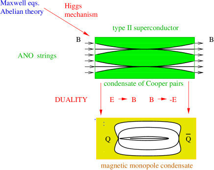
Figure 12: The QCD vacuum as a “dual” superconductor .

6.2.1 Abelian Higgs Model

A relativistic version of the Ginzburg–Landau model for superconductivity is the Abelian Higgs model:

$$L=-\frac{1}{4}F^{\mu\nu}F_{\mu\nu}+{1\over 2}(D^{\mu}\Phi)^{\dagger}(D_{\mu}\Phi)-U(\Phi)$$ (102)

where $\Phi$ is the Higgs field, in this case a complex (charged) scalar field describing Cooper pairs (i.e. condensate of electrons pairs in a lattice of positive ions, a superconducting solid) of charge $q=2e$, $e$ is the electron charge. $D_{\mu}\Phi=(\partial_{\mu}-iqA_{\mu})\Phi$ is the covariant derivative, and $U(\Phi)=\displaystyle\frac{\lambda^{\prime}}{4}(\Phi^{\dagger}\Phi-\mu^{2})^{2}$ is the Higgs potential. In Nielsen and Olesen (1973) it was shown that the Lagrangian (102) allows for vortex-line solutions. These vortex-lines solutions were approximately identified with the Nambu string.

The Lagrangian $L$ is invariant under local $U(1)$ transformations. However, if $\mu^{2}>0$, there is a condensation of Cooper pairs signalled by the vacuum expectation value $\langle\Phi\rangle\neq 0$. This corresponds to the spontaneous breaking of the U(1) electric symmetry. As a consequence the photon becomes massive inside a superconducting body and an external magnetic field can penetrate the body only to a finite depth $\lambda$ equal to the inverse of the photon mass (Meissner effect). In fact putting $\Phi=\rho e^{i\theta}$, $\rho>0$, and $\tilde{A}_{\mu}=(A_{\mu}-\partial_{\mu}\theta)$, $L$ can be rewritten in the gauge-invariant form

$$L=-\frac{1}{4}F^{\mu\nu}F_{\mu\nu}+\frac{M^{2}}{2}\tilde{A}^{\mu}\tilde{A}_{\mu}+{\tilde{L}}[\rho]$$ (103)

where ${\tilde{L}}$ is the sector of the Lagrangian describing the propagation of the massive field $\rho$ (mass $M_{\phi}$). The equations of motion for the electromagnetic field read

$$\partial^{\mu}F_{\mu\nu}+M^{2}\tilde{A}_{\nu}=0$$ (104)

with $M^{2}=q^{2}\langle\Phi\rangle^{2}$, the mass acquired by the photon.

In a stationary state with no charges $A_{0}=0$, $\partial_{0}{\bf A}=0$, Eq. (104) gives $({\bf H}=\nabla\wedge{\bf A})$

$$\nabla\wedge{\bf H}+M^{2}{\tilde{\bf A}} = 0$$ (105)

$$\nabla^{2}{\bf H}+M^{2}{\bf H} = 0$$ (106)

Eq. (105) means that a permanent current (London current) ${\bf j}=M^{2}{\tilde{\bf A}}$ exists, and since ${\bf E}=0$ and ${\bf E}=\sigma_{c}\,{\bf j}$ ($\sigma_{c}$ is the conductivity), $\sigma_{c}=0$.

The key parameter is the order parameter $\langle\Phi\rangle$ which signals the Higgs phenomenon. There are two characteristic lengths in the system related to $\langle\Phi\rangle$: the correlation length of the $\Phi$ field (or the inverse Higgs mass) $\Lambda=1/M_{\phi}$, $M_{\phi}=\lambda^{\prime}\langle\Phi\rangle$, and the penetration depth of the photon, $\lambda=1/M$. If $\lambda>\Lambda$ the superconductor is called of type II, and the formation of Abrikosov flux tubes is favored in the process of penetrating the material with a magnetic field. If the opposite inequality holds, $\lambda<\Lambda$, it happens that, when the magnetic field is increased, there is an abrupt penetration of it at some value and superconductivity is destroyed. The superconductor is of type I.

Summarizing, in this model the condensation of electric charges leads to the formation of a quantized flux tubes (see Exercise 6.2.1.1) whose radius and shape are controlled by $\Lambda$ and $\lambda$. If a magnetic monopole and antimonopole were introduced into such a superconducting medium they would be connected by a flux tube of finite energy per unit length (finite string tension). Thus magnetic monopoles would be confined due to a linear potential.

Exercises

• Show that a side consequence of the Meissner effect is the flux quantization. [Hint: Calculate the integral $\displaystyle\oint\tilde{\bf A}\cdot d{\bf x}$ around a large circle centered on the flux tube.]

• Consider the Maxwell equations in a relativistic medium without sources. Instead of expressing as usual the ${\bf E}$ and ${\bf B}$ fields in terms of the magnetic potential $A_{\mu}$, express the ${\bf D}=\varepsilon{\bf E}$ and ${\bf H}={\bf B}/\mu$ fields in terms of a (dual) electric potential $C_{\mu}$. Write down the Maxwell equations in a covariant form in terms of the field strength tensor of $C_{\mu}$. How do you have to modify the definition of this field strength tensor in the presence of sources?

b

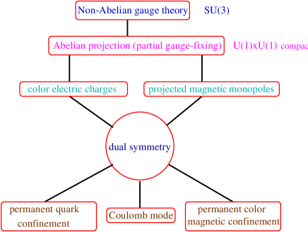
Figure 13: Schematic diagram illustrating how a Non-Abelian gauge theory reduces to an Abelian theory with electric charges and monopoles and the pattern of vacuum phases (see Sec. 4.4).

6.2.2 The QCD Vacuum

We have seen in the previous section how in ordinary superconductivity the condensation of electric charges gives origin to monopole confinement. On the other hand, in all the theories allowing for an analytic proof of electric charge confinement, like compact electrodynamics, the Georgi–Glashow model or some supersymmetric Yang–Mills theories (see Alvarez-Gaumé (1997)), this is due to the condensation of monopoles. However, if we want to apply this idea to QCD we have first to understand in which way we can obtain Abelian degrees of freedom and monopoles in QCD, since in the QCD Lagrangian there are no Higgs fields!. Subsequently we have to prove that the monopoles actually do condense. The application of this idea to non-Abelian gauge theories is based on the so-called Abelian projection, see ’t Hooft (1981). The Abelian projection is a partial gauge fixing (of the off-diagonal components of the gauge field) under which the Abelian degrees of freedom remain unfixed. In QCD the Abelian projection reduces the $SU(3)$ gauge symmetry to a $U(1)^{2}$ gauge symmetry. The Abelian projection monopoles appear as topological quantities in the residual Abelian channel. QCD is then reduced to an Abelian theory with electric charges and monopoles, see Fig. 13. Precisely, it can be regarded as an Abelian gauge theory with magnetic monopoles and charged matter fields (quarks and off-diagonal gluons). Then, the dual superconductor picture is realized if these Abelian monopoles condense: this causes confinement of the particles that are electrically charged with respect to the above “photons”. In this scenario large distance (low momentum) properties of QCD are carried by the Abelian degrees of freedom (Abelian dominance) and specifically by the monopole configurations (monopole dominance), see Suzuki (1993).

We do not have enough space to give further details. The reader is referred to Ex. 6.2.2.1 and to the reviews e.g. of Bali (1998), Chernodub et al. (1997), Di Giacomo (1998), Haymaker (1998). In the last years intensive work has been done to collect information on the quark confinement mechanism via lattice measurements. Depending on the picture, the excitations giving rise to confinement are thought to be magnetic monopoles, instantons, dyons, centre vortices (see Faber (1998)), etc. The above ideas are not completely disjoint and do not necessarily exclude each other. The above mentioned topological excitations indeed, are found to be correlated with each other in the lattice studies (e.g. correlations between instantons and monopoles). Many questions are still not completely settled. Here, we would like to summarize briefly the present understanding and to show some of the lattice measurements made in Abelian projection.

b

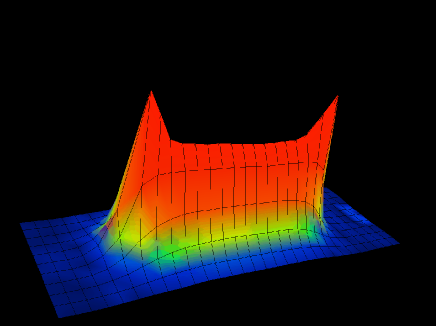
Figure 14: Action density distribution in Maximal Abelian Projection of $SU(2)$ measured on a lattice $V=32^{4}$ at $\beta=2.5115$. The physical quark-antiquark distance is $1.2$ fm. Figure provided by G. Bali.

First, we mention some general problems one encounters in this approach. 1) The identification of “photon fields” and monopoles is a gauge invariant process. However, the choice of the operator that defines the Abelian projection is somehow ambiguous. There are many different ways of making the Abelian projection. The physics, e.g. the monopole condensation, should be independent of the gauge fixing. 2) The actual composition of the condensate should be known. 3) The origin of the monopole potential that yields to a non-vanishing vacuum expectation value of the magnetic condensate should be understood.

On the other hand it is clear that: 1) monopoles are condensed in the confinement phase and this independently of the choice of the Abelian projection. 2) Monopoles are responsible for the main part of the nonperturbative dynamics. In particular Abelian and monopoles dominance seem to hold (in the Maximal Abelian Projection (MAP)): expectation values of physical quantities in the non-Abelian theory coincide with (or are very close to) the expectation values of the corresponding Abelian operators in the Abelian theory obtained via Abelian projection. In other words, disregarding the off-diagonal gluons, the long range features of a $SU(N)$ gauge theory are reproduced while short range features may be altered. Monopole dominance means that the same result can be approximately calculated in terms only of the monopole currents extracted from the Abelian fields.

b

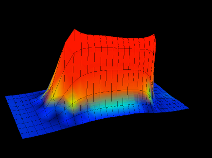
Figure 15: Monopole contribution to the action density distribution in Maximal Abelian Projection of $SU(2)$. Parameters as in Fig. 14.

As a general conclusion one can say that the lattice data in MAP show that the lattice gluodynamics is in a sense equivalent at large distances to the Dual Abelian Higgs model at the border between superconductor of type I and superconductor of type II. More precisely the Abelian monopole action has been extracted from $SU(2)$ lattice data in MAP and mapped into an Abelian Higgs model. From this the effective string theory has even been reconstructed and it occurs that the classical string tension of the string model is close to the quantum string tension of $SU(2)$ lattice gluodynamics, cf. Chernodub et al. (1999). The field distributions in MAP are found to satisfy the dual Ginzburg Landau equations and the coherence and the penetration lengths have been measured, cf. Bali (1998).

In Fig. 14 we present the action density distribution between two static quarks in $SU(2)$ in MAP to be compared on one hand with the action density in Fig. 11 and on the other hand with the monopole contribution in Fig. 15. We see that still the “photon” (neutral gluon) contributes to the self-energy of charges: the monopole part is free of self-energy while the “photon” part is free of string tension. Electric flux tubes (cf. Fig. 16) are found to be significantly thinner after Abelian projection.

b

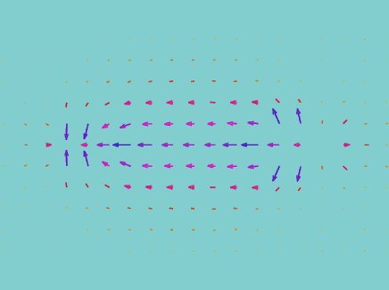
Figure 16: Electric field at 12 lattice units between two static quarks in $SU(2)$ measured on a lattice $V=32^{4}$ at $\beta=2.5115$. The lattice spacing is fixed on $\sigma=(440$ MeV$)^{2}$. The physical quark-antiquark distance is 1 fm. Figure provided by G. Bali.

At the end of this section we present two plots of the static potential. Fig. 17 is a plot of the static potential calculated by means of either non-Abelian or Abelian projected Wilson loops. If one takes into account that in the Abelian projected case all the “charged components” of $A_{\mu}$ are neglected, one finds an impressive agreement between the two curves. Fig. 18 shows the static potential calculated in the Abelian projection. The photon contribution and the monopole contribution have been calculated separately. This plot confirms the action density result discussed above. Moreover, it is possible to quantify $\sigma_{U(1)}\simeq 92\%\,\sigma_{SU(2)}$ and $\sigma_{mon}\simeq 95\%\,\sigma_{U(1)}$. Notice that in the Abelian projection the coefficient of the Coulombic part comes out to be smaller by more than a factor of two.

The original phenomenological Cornell potential that was confirmed by the lattice simulations on the static Wilson loop in Sec. 4.5, is now understood in terms of monopole contributions while the monopole currents are the origin of the chromoelectric flux tube.

It is also possible to construct infrared effective “analytic” models based upon the assumptions and on the results presented above and to use them to explain the QCD low energy physics. As already discussed, in the Wilson loop formalism only an assumption on the Wilson loop behaviour is necessary. This is outlined in the next sections.

b

Figure 17: Static potential in $SU(2)$ (diamonds) and in the Abelian projection of $SU(2)$ (squares) (in lattice units, $a\simeq 0.081$ fm). Bali et al. (1996).

b

Figure 18: The Abelian projected $SU(2)$ potential (diamonds) in comparison with the “photon” contribution (squares), the monopole contribution (crosses) and the sum of the two parts (triangles) (in lattice units, $a=0.081$ fm). No self-energy constant have been subtracted. Bali et al. (1996).

Exercises

• This is a simple example of Abelian projection for SU(2). Consider the following condition $F_{12}(x)=\hbox{diagonal matrix}$. Show that $F_{12}$ is still invariant under the U(1) gauge transformation $\Omega(x)_{ij}$ defined as

  $$\Omega_{12}=\Omega_{21}=0\qquad\Omega_{11}=\Omega_{22}^{*}=e^{i\alpha(x)}\qquad\alpha\in[0,2\pi).$$

  Define $A_{\mu}^{\pm}\equiv A_{\mu}^{1}\pm A_{\mu}^{2}$, $1,2,3=$ colour indices. Show that $A_{\mu}^{3}$ transforms as a photon under $\Omega$ while $A_{\mu}^{\pm}$ transform as charged fields. Define an Abelian field strength tensor in terms of $A_{\mu}^{3}$ and show that, if the matrix of the gauge transformation $\Omega$ contains singularities, also the Abelian field strength tensor may contain singularities (monopoles).

6.3 Low energy theorems and flux tube

We have seen that one of the relevant features of confinement is the interquark flux tube formation, see Figs. 11, 16 in $SU(2)$ and Figs. 14, 15 in the MAP of $SU(2)$. Typical quantities of interests are the transverse extent of the flux tube and the nature of the colour fields (i.e. electric or magnetic), see Bali et al. (1995) and Green et al. (1997). There are two low energy theorems relating the potential of a static quark-antiquark pair with the total energy and the action stored in the flux tube between the sources (in lattice QCD these are know as Michael’s sum rules (Michael (1987)), Dosch et al. (1995), Novikov et al. (1981), Shifman (1998),

$$V_{0}(r) = {1\over 2}\langle\int d^{3}x(-{\bf E}(x)^{2}+{\bf B}(x)^{2})\rangle_{r\times T}$$

$$V_{0}(r)+r{\partial V_{0}(r)\over\partial r} = {1\over 2}{\beta({\alpha_{\rm s}})\over\alpha_{\rm s}}\langle\int d^{3}x({\bf E}(x)^{2}+{\bf B}(x)^{2})\rangle_{r\times T}.$$ (107)

$\langle\cdots\rangle_{r\times T}$ denotes the expectation value in the presence of the static Wilson loop where the expectation value in the absence of the sources has been subtracted. The formulas are in Euclidean space and renormalized composite operators are used. The squared electric and magnetic field strengths are separately not renormalization group invariant. Thus statements like $\langle g^{2}{\bf B}^{2}\rangle_{r\times T}\simeq 0$ or $\langle g^{2}{\bf E}_{\perp}^{2}\rangle_{r\times T}\simeq 0$ are scale dependent. As we already pointed out, on the lattice the averages of the squared components of the colour fields are found to be roughly equal (i.e. $\langle E_{i}^{2}\rangle_{r\times T}$ $\simeq$ $\langle B^{2}_{j}\rangle_{r\times T}$, $i,j=1,2,3$), while in the greater part of the models the flux tube is mainly made of the longitudinal electric field. Eqs. (107) fixes the scale at which each of these situations can be fulfilled. In particular for models, typically describing the long range behaviour with $V_{0}\simeq\sigma r$, one has $\beta/\alpha_{\rm s}\simeq-2$. Taking the three-loop beta function, this gives $\alpha_{\rm s}\simeq 0.6$.

6.4 Models of the QCD Vacuum

We briefly mention some analytic models of the QCD vacuum. We refer the reader to the papers quoted below for further details.

b

Figure 19: On a semi-log scale, a comparison of the total energy profile for dual QCD (solid line) and in the lattice predictions (solid circles) for $R$ (=$q\bar{q}$ distance) ranging from 8 down to 1 lattice units as a function of the transverse coordinate $r_{\rm T}$ (with respect to the interquark string). All profiles are in lattice units with $a\simeq 0.6$ $Gev^{-1}$. From Green et al. (1997).

6.4.1 Dual QCD (DQCD)

Impressive progresses have been done recently towards an understanding of confinement via duality and monopoles condensation in supersymmetric theories, see e.g. Alvarez-Gaumé et al. (1997). However, it is also possible to construct a dual effective theory of long distance Yang–Mills theory, Baker et al. (1986-1996), see also Maedan et al. (1989). We call this theory Dual QCD (DQCD).

DQCD is a concrete realization of the Mandelstam and ’t Hooft dual superconductor mechanism of confinement. It describes the QCD vacuum as a dual superconductor on the border between type I and II. The Wilson loop approach supplies a simple method to connect averaged local quantities in QCD and in dual QCD. For large loops we assume

$$\langle W(\Gamma)\rangle\simeq{\displaystyle{\int\!{\cal D}{C}\,{\cal D}{B}\,\exp\left[i\int dxL(G_{\mu\nu}^{\rm S})\right]}\over\displaystyle{\int\!{\cal D}{C}\,{\cal D}{B}\,\exp\left[i\int dxL(0)\right]}}$$ (108)

where $L$ is the effective dual Lagrangian. The fundamental variables are an octet of dual potential $C_{\mu}$ coupled minimally to three octets of scalar Higgs field $B_{i}$ carrying magnetic colour charge, the dual coupling constant being $e=2\pi/g$. Notice that the dual transformation exchange the strong coupling limit of QCD with the weak coupling limit of DQCD. The monopole fields $B_{i}$ develop nonvanishing expectation values $B_{0i}$ giving rise to massive $C_{\mu}$ and to a dual Meissner effect. Dual potentials couple to electric colour charges like ordinary potentials couple to monopoles, i.e. $C_{\mu}$ couple to the quark-antiquark pair via a Dirac string connecting the pair. It turns out that, for the description of a quark-antiquark state, the relevant subset of the theory is a (dual) Abelian Higgs model. In this case indeed, the effective Lagrangian is explicitly given by ${L}(G_{\mu\nu}^{\rm S})=2~{}{\rm Tr}\{-{1\over 4}{G}^{\mu\nu}{G}_{\mu\nu}$ $+{1\over 2}({D}_{\mu}{B}_{i})^{2}\}-U({B}_{i})$, where $G_{\mu\nu}=(\partial_{\mu}C_{\nu}-\partial_{\nu}C_{\mu}+G^{S}_{\mu\nu})$. The dual field is directed along the hypercharge matrix $Y$ in the colour space, $G_{\mu\nu}^{\rm S}(x)=g\,\epsilon_{\mu\nu\alpha\beta}\displaystyle\int ds\int d\tau\,\displaystyle{\partial y^{\alpha}\over\partial s}{\partial y^{\beta}\over\partial\tau}\delta(x-y(s,\tau))\,Y$, ($y(s,\tau)$ is a world sheet with boundary $\Gamma$ swept out by the Dirac string) and $U({B}_{i})$ is the Higgs potential with the minimum values $B_{0i}$ chosen in order to completely break the dual $SU(3)$ symmetry. It essentially coincides with the Abelian Higgs Lagrangian (plus sources) of Eq. (102) where the fields $A_{\mu}$ play the role of the dual potentials $C_{\mu}$ and a combination of fields $B_{i}$ plays the role of the Higgs field $\Phi$.

From (108) it follows that (see Baker et al. (1996))

$$\langle\!\langle F_{\mu\nu}(z_{j})\rangle\!\rangle={2\over 3}\,\varepsilon_{\mu\nu\rho\sigma}\langle\!\langle G^{\rho\sigma}(z_{j})\rangle\!\rangle_{Dual}\,.$$ (109)

Therefore, it is possible to relate averaged values of local quantities in QCD and in the dual theory. The nonperturbative parameters are the v.e.v. of the Higgs field and the coupling constant of the Higgs potential (from these the penetration length and the correlation length can be constructed). Flux tube configurations with finite $r_{MS}\sim{1/M}$, $M=$ mass of the dual gluon, arise (Baker et al. (1996)) from the numerical solution of the classical dual Ginzburg–Landau type of equations obtained from $L$. The flux tube profile agrees well with lattice data (Green et al. (1996)), see Fig. 19. It is the presence of the Higgs field which confines the transverse energy distribution in a flux tube. The string tension $\sigma$ comes from the integral of the exponentially decreasing energy distribution.

b

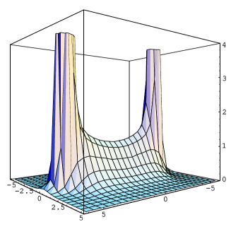
Figure 20: The energy density distribution in GeV/$fm^{3}$ caused by the nonperturbative correlator $D$ and the colour Coulomb contribution $D_{1}$ with $\alpha_{s}=0.57$. In the figure $a=T_{g}=0.35fm$, the $q\bar{q}$ distance is 9 $T_{g}$. From Rüter et al. (1995).

6.4.2 Stochastic Vacuum Model

The Stochastic Vacuum Model (Dosch (1987), Dosch et al. (1988)) is based on the idea that low frequency contributions in the functional integral can be taken into account by a simple stochastic process with a converging cluster expansion. Under this assumption the Wilson loop manifests an area law behaviour and therefore linear confinement. The model does not give rise to confinement for an Abelian gauge theory. In order to make quantitative predictions it is convenient to make a more radical assumption, namely that all higher cumulants can be neglected as compared to the two point function. This assumption appears to be in agreement with a recent lattice analysis (Bali et al. (1998)). Then, the stochastic process is Gaussian and all fields correlators are reduced to products of two point functions by factorization. This means that the Wilson loop can be approximated simply by (in Euclidean space)

$$\langle W(\Gamma)\rangle\simeq\exp\left[-\displaystyle{g^{2}\over 2}\int_{S(\Gamma)}\!\!\!\!dS_{\mu\nu}(x)\int_{S(\Gamma)}\!\!\!\!dS_{\lambda\rho}(y)\langle F_{\mu\nu}(x)U(x,y)F_{\lambda\rho}(y)U(y,x)\rangle\right]$$ (110)

where $S(\Gamma)$ is a surface with contour $\Gamma$, typically the minimal area surface. The nonperturbative dynamics is given in terms of one unknown function only: the non-local gluon condensate

$$g^{2}\langle U(0,x)F_{\mu\nu}(x)U(x,0)F_{\lambda\rho}(0)\rangle=\bigg{\{}(\delta_{\mu\lambda}\delta_{\nu\rho}-\delta_{\mu\rho}\delta_{\nu\lambda})(D(x^{2})+D_{1}(x^{2}))$$

$$+(x_{\mu}x_{\lambda}\delta_{\nu\rho}-x_{\mu}x_{\rho}\delta_{\nu\lambda}+x_{\nu}x_{\rho}\delta_{\mu\lambda}-x_{\nu}x_{\lambda}\delta_{\mu\rho}){d\over dx^{2}}D_{1}(x^{2})\bigg{\}}.$$ (111)

Eq. (111) is the most general Lorentz decomposition of the two-point correlator. The dynamics is contained in the form factors $D$ and $D_{1}$. The function $D$ is responsible for the area law and confinement.

Lattice simulations (for a sum-rule analysis see Dosch, Eidemüller and Jamin (1998)) show that the $D$ and $D_{1}$ functions exhibit a long-range exponential fall off $\simeq F_{2}\exp\{-|x|/T_{g}\}$ where the correlation length $T_{g}$ is about 0.2 $\div$ 0.3 fm (D’Elia et al. (1997)). The model has thus two nonperturbative parameters $F_{2}$ and $T_{g}$. The static potential is given by

$$V_{0}(r)\simeq F_{2}\int_{0}^{\infty}d\tau\int_{0}^{r}d\lambda\,(r-\lambda)D(\tau^{2}+\lambda^{2})$$ (112)

and the string tension $\sigma$ emerges as an integral on the function $D$, $\sigma\simeq F_{2}\displaystyle\int_{0}^{\infty}d\tau$ $\displaystyle\int_{0}^{\infty}d\lambda$ $D(\tau^{2}+\lambda^{2})$, in the limit ${T_{g}/r}\to 0$. The field distribution between the quark and the antiquark is a flux tube (Rüter et al. (1995)) with $r_{MS}\simeq 1.8\,T_{g}$, see Fig. 20. We refer to Dosch (1994), Nachtmann (1996) and Simonov (1996) for a complete description of the model and its applications.

Finally, we mention in this neither exhaustive nor complete list, the flux tube model of Isgur et al. (1983). This model is extracted from the strong coupling limit of the QCD lattice Hamiltonian. A $N$-body discrete string-like Hamiltonian describes the gluonic degrees of freedom. The limit $N\to\infty$ corresponds to a localized string with an infinite number of degrees of freedom.

All the mentioned models allow to obtain via Eqs. (73), (81), (82), the complete semirelativistic quark interaction. For a discussion and a comparison of the result see Baker et al. (1997), Brambilla et al. (1997a) and Brambilla (1998). A relation between DQCD and SVM has been established in Baker et al. (1998).

Here, we only stress that we need two parameters like $T_{g}$ and $F_{2}$ to control the structure of the flux tube. Had we only one parameter, like the string tension $\sigma$, we could only encode the information of a constant energy density in the flux tube. However, the whole structure is important and also the information about the width of the flux tube (typically proportional to $T_{g}$) has to be considered.

Exercises

• Show that in the limit $T_{g}\to 0$ the Wilson loop in Eq. (110) is given by $\exp\{-\sigma S\}$ with $\sigma$ as defined above and $S$ the surface enclosed by the loop $\Gamma$.

• Show that using the lattice parameterization of $D$ given above, with $T_{g}\simeq 0.3$ fm and $F_{2}\simeq 0.048$ GeV⁴, the Stochastic Vacuum Model gives a string tension $\sigma$ compatible with the phenomenological value of Eq. (5).

6.5 String description of QCD

An effective string theory of strong interaction has been proposed first by Nambu and Goto in 1960 to explain the fact that the hadrons lie on Regge trajectories (see Sec. 2). Nambu was the first who explicitly constructed an effective theory of the Abelian Higgs model working in the limit of infinite Higgs mass which turned out to be coincident with the Nambu–Goto string Lagrangian. Recent works have shown that properly summing over all the string positions to account for the fluctuation of the string generates an effective string in four dimension free of the conformal anomaly. Results exist both in the limit of infinite Higgs mass (Akhmedov et al. (1996)) and without taking that singular limit (Baker et al. (1999)). A phenomenological description of hybrids has been obtained using a Nambu–Goto action in Allen et al. (1998).

7 Summary

These lectures have been devoted to a summary of our understanding of the heavy hadron spectrum in QCD. We started from some phenomenological guess of the interquark static potential inspired from a naive flux tube picture. Then, we managed to give a well founded definition of such a potential in field theory and to “derive” the quark confinement property in strong coupling expansion. To obtain the form of the potential we resorted to the lattice formulation and to numerical techniques that eventually confirmed the linear rising of the phenomenological static potential. The relativistic corrections were added in the framework of effective field theories establishing a systematic way of estimating the neglected terms. This allowed us to obtain a gauge-invariant field theory based definition of the semirelativistic quark interaction devised for lattice simulations as well as for analytic calculations. Eventually this procedure enabled us to connect directly the QCD vacuum with the spectrum. At the end we examined the Wilson loop in the Abelian projection suggested by ’t Hooft, i.e. under the assumption that the QCD vacuum is a dual superconductor, and we found that our initial Cornell potential seems to be the output of dominant monopoles configurations.

The aim of these lectures has been to show how heavy quark bound states offer an ideal situation where exact results from QCD (effective field theories like NRQCD and pNRQCD) can be used to explore the QCD vacuum either with lattice numerical tools or by means of analytic models. Therefore many theoretical ideas and techniques can be and have been used in order to explain that kind of systems. All of them cooperate to enlarge our predictability and to open new perspectives. It is not surprising that, in spite of several still open problems, some remarkable progress have been achieved.

References

References

- [1] A. Abrikosov, JETP 32, 1442 (1957).
- [2] T. Allen, M. G. Olsson and S. Veseli, Phys. Lett. B 434, 100 (1998); hep-ph/9810363.
- [3] L. Alvarez-Gaumé, F. Zamora, (Lectures) hep-th/9709180.
- [4] E. T. Akhmedov, M. N. Chernodub, M. I. Polikarpov and M. A. Zubkov, Phys. Rev. D 53, 2087 (1996).
- [5] G. S. Bali, C. Schlichter and K. Schilling, Phys. Rev. D 51, 5165 (1995).
- [6] G. S. Bali, V. G. Bornyakov, M. Müller–Preussker and K. Schilling, Phys. Rev. D 54, 2863 (1996).
- [7] G. S. Bali, A. Wachter and K. Schilling, Phys. Rev. D 56, 2566 (1997); G. Bali and Boyle, hep-lat/9809180.
- [8] G. S. Bali, N. Brambilla and A. Vairo, Phys. Lett. B 421, 265 (1998).
- [9] G. S. Bali, hep-ph/9809351.
- [10] M. Baker, J. S. Ball and F. Zachariasen, Phys. Lett. B 152, 351 (1985).
- [11] M. Baker, J. Ball and F. Zachariasen, Phys. Rev. D 51, 1968 (1995); Phys. Rev. D 44, 3328 (1991).
- [12] M. Baker, J. S. Ball and F. Zachariasen, Int. Jour. Mod. Phys. A11, 343 (1996a).
- [13] M. Baker, J. S. Ball, N. Brambilla, G.M. Prosperi and F. Zachariasen, Phys. Rev. D 54, 2829 (1996b); M. Baker, J. S. Ball, N. Brambilla, A. Vairo, Phys. Lett. B 389, 577 (1996b).
- [14] M. Baker, J. S. Ball and F. Zachariasen, Phys. Rev. D 56, 4400 (1997).
- [15] M. Baker, N. Brambilla, H. G. Dosch and A. Vairo, Phys. Rev. D 58, 034010 (1998).
- [16] M. Baker and R. Steinke, in preparation (1999).
- [17] A. Barchielli, E. Montaldi and G. M. Prosperi, Nucl. Phys. B 296, 625 (1988); Erratum ibid. B 303, 752 (1988).
- [18] A. Barchielli, N. Brambilla and G. M. Prosperi, Nuovo Cimento 103 A, 59 (1990).
- [19] I. Bigi, Y. Dokshitzer, V. Khoze, J. Kuhn and P. Zerwas, Phys. Lett. B 181, 157 (1986).
- [20] N. Brambilla and G. M. Prosperi, Phys. Lett. B 236, 69 (1990).
- [21] N. Brambilla and G. M. Prosperi, Phys. Rev. D 48, 2360 (1993); Phys. Rev. D 46, 1096 (1992).
- [22] N. Brambilla, P. Consoli, G. M. Prosperi, Phys. Rev. D 50, 5878 (1994).
- [23] N. Brambilla and A. Vairo, Phys. Rev. D 55, 3974 (1997a).
- [24] N. Brambilla and A. Vairo, Phys. Lett. B 407, 167 (1997b).
- [25] N. Brambilla and A. Vairo, hep-ph/9809230; A. Vairo, hep-ph/9809229.
- [26] N. Brambilla, hep-ph/9809263.
- [27] N. Brambilla, A. Pineda, J. Soto, A. Vairo, hep-ph/9903355 and in preparation.
- [28] L. S. Brown and Weisberger, Phys. Rev. D 20, 3239 (1979).
- [29] W. Buchmüller and S. H. Tye, Phys. Rev. D 24, 132 (1981).
- [30] W. Buchmüller, Phys. Lett. B 112, 479 (1982).
- [31] S. Capitani, M. Lüscher, R. Sommer and H. Wittig, hep-lat/9810063 and refs. therein.
- [32] Yu-Qi Chen, Yu-Ping Kuang and R. J. Oakes, Phys. Rev. D 52, 264 (1995) 264; Yu-Qi Chen and Yu-Ping Kuang, Z. Phys. C 67, 627 (1995). Some errors related to the reparameterization invariance where corrected in M. Finkemeier, H. Georgi and M. McIrvin, Phys. Rev. D 55 6933 (1997).
- [33] M. Chernodub and M. Polikarpov, (Lectures) hep-th/9710205.
- [34] M. Chernodub, S. Kato, N. Nakamura and M. Polikarpov, hep-lat/9902013.
- [35] M. Creutz and K. Moriarty, Phys. Rev. D 26, 2166 (1982).
- [36] M. Creutz, Quarks, gluons and lattices, (Cambridge University Press, Cambridge, 1983).
- [37] C. Davies, Lectures given at the 1997 Schladming School, Schladming, Austria, (Springer, Berlin, 1997).
- [38] A. Di Giacomo, hep-lat/9802008.
- [39] H. G. Dosch, Phys. Lett. B 190, 177 (1987).
- [40] H. G. Dosch and Yu. A. Simonov, Phys. Lett. B 205, 339 (1988).
- [41] H. G. Dosch, Prog. Part. Nucl. Phys. 33, 121 (1994); H. G. Dosch, E. Ferreira and A. Krämer, Phys. Rev. D 50, 1992 (1994).
- [42] H. G. Dosch, O. Nachtmann and M. Rüter, hep-ph/9503386.
- [43] H. G. Dosch and S. Narison, Phys. Lett. B 417, 173 (1998).
- [44] H. G. Dosch, M. Eidemüller and M. Jamin, hep-ph/9812417.
- [45] M. D’Elia, A. Di Giacomo and E. Meggiolaro, Phys. Lett. B 408, 315 (1997) and refs. therein.
- [46] E. Eichten, K. Gottfried, T. Kinoshita, K. D. Lane and T. M. Yan, Phys. Rev. D 17, 3090 (1978); D 21, 203 (1980).
- [47] E. Eichten and F. Feinberg, Phys. Rev. D 23, 2724 (1981).
- [48] M. Faber, J. Greensite and S. Olejnik, hep-lat/9810008 and refs. therein.
- [49] S. Godfrey and N. Isgur, Phys. Rev. D 32 189 (1985).
- [50] S. Godfrey and J. Napolitano, hep-ph/9811410.
- [51] A. M. Green, C. Michael and P. S. Spencer, Phys. Rev. D 55, 1216 (1997).
- [52] D. Gromes, Phys. Lett. B 115, 482 (1982).
- [53] D. Gromes, Z. Phys. C 26, 401 (1984); 22 265 (1984).
- [54] D. J. Gross and F. Wilczek, Phys. Rev. Lett. 30, 1343 (1973).
- [55] R. W. Haymaker, to be published in Phys. Rep., hep-lat/9809094.
- [56] N. Isgur, Phys. Rev. D 57, 4041 (1998).
- [57] N. Isgur and J. Paton, Phys. Lett. B 124, 247 (1983); N. Isgur and J. Paton, Phys. Rev. D 31, 2910 (1985).
- [58] M. Jamin and A. Pich, hep-ph/9810259.
- [59] R. D. Kenway, hep-lat/9810054.
- [60] J. Kogut, R. Pearson and J. Shigemitsu, Phys. Lett. B 98, 63 (1981).
- [61] G. P. Lepage and P. Mackenzie, Phys. Rev. D 48, 2250 (1993).
- [62] G. P. Lepage, Lectures given at the 1996 Schladming School, Schladming, Austria, (Springer, Berlin, 1996).
- [63] H. Leutwyler, Phys. Lett B 98, 447 (1981).
- [64] H. Leutwyler, Phys. Lett. B 378, 313 (1996).
- [65] W. Lucha, F. F. Schöberl and D. Gromes, Phys. Rep. 200, 127 (1991).
- [66] S. Maedan and T. Suzuki, Prog. Theor. Phys. 81, 229 (1989).
- [67] S. Mandelstam, Phys. Rep. C 23, 245 (1976).
- [68] S. Mandelstam, Phys. Rev. D 19, 2391 (1979).
- [69] A. Manohar, Phys. Rev. D 56, 230 (1997).
- [70] A. Martin, Phys. Lett. B 93, 338 (1980).
- [71] R. McClary and N. Byers, Phys. Rev. D 28, 1692 (1983).
- [72] C. Michael, Nucl. Phys. B 280, 13 (1987).
- [73] C. Michael, hep-ph/9710429; hep-ph/9809211.
- [74] C. Morningstar, K. J. Juge and J. Kuti, hep-ph/9809015.
- [75] I. Montvay and G. Munster, Quantum fields on a lattice, (Cambridge Univ. Press, Cambridge, 1994).
- [76] O. Nachtmann, Lectures given at the 1996 Schladming School, Schladming, Austria, (Springer, Berlin, 1996).
- [77] Y. Nambu, Phys. Rev. D 10, 4262 (1974).
- [78] H. B. Nielsen and P. Olesen, Nucl. Phys. B 61, 45 (1973).
- [79] V. A. Novikov, M. A. Shifman, A. I. Vainshtein, V. I. Zakharov, Nucl. Phys. B 191, 301 (1981).
- [80] M. G. Olsson and K. Williams, Phys. Rev. D 48, 417 (1993); M. G. Olsson and S. Veseli, Phys. Rev. D 51, 3578 (1995); M. G. Olsson, Int. J. Mod. Phys. A 12, 4099 (1997).
- [81] PDG (1998), Particle data Group. See review of particle Physics C. Caso et al., The European Physical Journal C 3 1 (1998) or http://pdg.lbl.gov/.
- [82] M. A. Peskin, in Proc. 11th SLAC Summer Institute, PUB-3273, (SLAC, 1983).
- [83] M. Peter, Nucl. Phys. B 501, 471 (1997).
- [84] A. Pineda and F. J. Yndurain, hep-ph/9812371 and refs. therein.
- [85] A. Pineda and J. Soto, Nucl. Phys. B (Proc. Suppl.) 64, 428 (1998); Phys. Rev. D 59, 016005 (1999).
- [86] H. D. Politzer, Phys. Rev. Lett. 30, 1346 (1973).
- [87] C. Quigg, Physics Today 50, 20 (1997).
- [88] C. Quigg and J. L. Rosner, Phys. Lett. B 71, 153 (1977).
- [89] J. Richardson, Phys. Lett. B 82, 272 (1979).
- [90] H. Rothe, Lattice gauge theories. An Introduction, (World Scientific, Singapore, 1992).
- [91] M. Rüter and H. G. Dosch, Z. Phys. C 66, 245 (1995).
- [92] J. J. Sakurai, Modern Quantum Mechanics, (The Benjamin/Cummings Pub. Comp., 1985).
- [93] Y. Schröder, Phys. Lett. B 447, 321 (1999) where an error in Peter (1997) is corrected.
- [94] H. J. Schitzner, Phys. Lett. B 76, 461 (1978).
- [95] M. Shifman, A. Vainshtein and V. Zakharov, Nucl. Phys. B 147, 385 (1979); ib. 448.
- [96] M. Shifman, Prog. Theor. Phys. Suppl. 131, 1 (1998).
- [97] Yu. Simonov, Phys. Usp. 39, 313 (1996).
- [98] T. Suzuki, Nucl. Phys. B (Proc. Suppl.) 30, 176 (1993).
- [99] R. Tafelmayer, Diploma Thesis, Heidelberg (1986).
- [100] G. ’t Hooft, in High Energy Physics, ed. Zichichi (Editrice Compositori, Bologna, 1976).
- [101] G. ’t Hooft, Nucl. Phys. B 153, 141 (1979).
- [102] G. ’t Hooft, Nucl. Phys. B 190[FS3], 455 (1981).
- [103] G. ’t Hooft, Physica Scripta 25, 133 (1982).
- [104] G. ’t Hooft, Under the spell of the gauge principle, (World Scientific, Singapore, 1994).
- [105] B. Thacker and G. Lepage, Phys. Rev. D 43, 196 (1991); G. P. Lepage, L. Magnea, C. Nakhleh, U. Magnea and K. Hornbostel, Phys, Rev. D 46, 4052 (1992).
- [106] M. B. Voloshin, Nucl. Phys. B 154, 365 (1979).
- [107] S. Weinberg, Prog. of Theor. Phys. Suppl. 86, 43 (1986).
- [108] F. J. Wegner, J. Math. Phys. 12, 2259 (1971).
- [109] K. Wilson, Phys. Rev. D 10, 2445 (1974).