SHEP 99/03
hep-ph/9904315
Preheating in Supersymmetric Hybrid Inflation
M. Bastero-Gil, S. F. King and J. Sanderson
Department of Physics and Astronomy, University of Southampton,
Southampton, SO17 1BJ, U.K.
ABSTRACT
We study preheating in a general class of supersymmetric hybrid inflation model. Supersymmetry leads to only one coupling constant in the potential and thus only one natural frequency of oscillation for the homogeneous fields, whose classical evolution consequently differs from that of a general (non-supersymmetric) hybrid model. We emphasise the importance of mixing effects in these models which can significantly change the rate of production of particles. We perform a general study of the rate of production of the particles associated with the homogeneous fields, and show how preheating is efficient in producing these quanta. Preheating of other particle species will be model dependent, and in order to investigate this we consider a realistic working model of supersymmetric hybrid inflation which solves the strong-CP problem via an approximate Peccei-Quinn symmetry, which was proposed by us previously. We study axion production in this model and show that properly taking into account the mixing between the fields suppresses the axion production, yet enhances the production of other particles. Finally we demonstrate the importance of backreaction effects in this model which have the effect of shutting off axion production, leaving the axion safely within experimental bounds.
1 Introduction
Reheating in the post-inflationary Universe is a very important process, since it describes the formation of all matter and energy in the Universe today [1]. However, it has only relatively recently [2] been realised that in certain cases the process of reheating involves a stage of explosive production of particles by parametric resonance which cannot be described by the usual methods of the elementary reheating theory [3]. This stage of ‘preheating’ is a non-perturbative and out of equilibrium process and as such is a very involved and little understood proceeding. In fact there have been complex analytical methods of preheating developed for only the very simplest of single-field inflationary potentials [4]. It is generally numerically easy to obtain results for the first stages of particle production, yet a complete, self-consistent analysis should include all effects of backreaction of produced particles and their rescattering. At present lattice simulations (such as in [5, 6]) must be performed to fully study these effects. Nevertheless, much progress is being made in developing methods to cope with the rich topic of preheating [4].
For a while now, the advantages of using more than one scalar field to implement inflation have been well appreciated. Hybrid inflation models [7] are probably the most popular of all present inflationary models. They succeed in removing the need for fine-tuning of the inflaton potential by providing a natural means to end inflation. Most importantly however, they allow inflation to occur at a relatively low energy density using small scale fields avoiding strong CMB constraints, a task which is virtually impossible to achieve using only one field. Thus, hybrid-type models are attractive from the point of view of particle physics and in particular are naturally well suited to realisations in supersymmetry (SUSY) where there is an abundance of scalar fields and flat directions.
Preheating in hybrid inflation has been studied [8] using the standard toy hybrid potential of two fields , coupled to an extra, massless scalar field, by the interaction . It is found [8] that over most of the parameter space, preheating is rather inefficient in hybrid inflation with little production of particles although production of particles is possible for certain values of . However, the results concerning the production of and particles may change in a supersymmetric version of the model, where the potential is derived from a supersymmetric superpotential of the kind , such that the same coupling will give the quartic self-interaction for the field and the interaction term between and the inflaton . Therefore, supersymmetry will ensure that the masses of both fields at the global minimum of the potential are not only the same order of magnitude but . This in turn will give rise to a non-chaotic evolution of the classical homogeneous fields at the beginning of the preheating/reheating era. The classical fields will begin to oscillate with relatively large, little damped amplitudes, which will favour production of particles occurring.
In addition, in hybrid models inflation ends with a phase transition when the inflaton field reaches a critical value. At this point, the second field is sited at a maximum of the potential with vanishing mass. Once the inflaton passes this point, the mass of becomes negative allowing both fields to roll down the potential towards the global minimum. It is clear that across the region of the spinodal instability (negative curvature) [9], production of particles can be quite intensive. Therefore, previous to any oscillation of the homogeneous fields, preheating will begin with an initial burst of production. If the amplitude of the oscillations is large enough, this will also happen in the successive oscillations every time the classical fields enter the region of the spinodal instability. Although this only directly affects the rate of production of particles, the effect is propagated into the production of particles through the mixing term in the mass squared matrix.
The layout of the paper is as follows: section 2 briefly describes the theory of preheating as applied to many scalar fields and we point out that the coupling between fields should in general be taken into account; in section 3 we study a general model of supersymmetric hybrid inflation, focusing on the issue of production of and particles; in order to motivate production of other particles, which is model dependent, in section 4 we review a particular model of inflation where the strong-CP problem is solved via a Peccei-Quinn symmetry which leads to the production of axions. It will be important to calculate the effects of preheating in this model since the number of axions produced during reheating must be tightly constrained in order to be cosmologically acceptable. The results of the numerical study of the first stages of preheating in this model are presented, and compared to those results without including mixing terms. The first effects of backreaction of produced particles is studied and the total number of each type of particle calculated.
2 Theory of preheating with multiple fields
We begin with a model of the early Universe described by a potential, , in an expanding Universe with scale factor . Amongst the fields in the potential, there are degrees of freedom corresponding to scalar fields in which all energy is concentrated during inflation. In the usually considered single-field inflation this is the slowly rolling inflaton, , with effective potential . In the hybrid scenario there are two such fields important to inflation, one in which the potential is relatively flat during inflation which acts as the inflaton field, , and one which sits in a false vacuum, , and causes the end of inflation in the phase transition to its true vacuum. All other fields are not important to inflation serving only perhaps to provide the constant vacuum energy during inflation.
In order to investigate the reheating of the Universe and determine the extent of the effects of preheating, we must first study the evolution of these fields as inflation ends and beyond into the regime of coherent oscillations.
We may write the full quantum fields as:
| (1) |
where represents the quantum fluctuations about the homogeneous zero modes, , and necessarily satisfies .
Neglecting ensuing effects of particle production, we proceed by considering the motion classically, solving the equations of motion for the classical homogeneous fields , but using quantum fluctuations (where is the Hubble constant during inflation) in the initial conditions at the end of inflation to initiate the spontaneous symmetry breaking.
The equations of motion governing the behaviour of the background fields, , are:
| (2) |
where the Hubble constant is given by the Friedmann equation,
| (3) |
and .
Here, the subscript runs over all the classical scalar fields in the theory relevant to inflation and is the effective potential of these fields. During inflation all energy is contained in this potential and the Universe is in a vacuum-like state with vanishing temperature, entropy and particle number densities. The inflaton field, , is slowly rolling with the friction term dominating in Eq. (2) so that:
| (4) |
This also describes the relevant situation for each classical field at the beginning of the reheating era.
The equations of motion for the quantum fluctuations of the scalar fields in linear perturbation theory are given by:
| (5) |
where are the time dependent Fourier modes (in comoving momentum space k) of the quantum fluctuations ,
| (6) |
and and are creation and annihilation operators. Thus, Eq. (5) describes the interactions between the classical fields, , and the quantum fluctuations, . When neglecting backreaction effects due to the particles produced, the Hubble constant, , and the mass squared matrix, , are functions of the classical fields only, as given by the classical equations of motion (2) and (3). It should be clear that the equations of motion for the quantum fluctuations will in general be coupled through mixing terms in the mass matrix (for ); in other words the rate of production of each separate particle is dependent on the rate of production of the others, even at the initial stage of preheating when backreaction effects are not yet important.
Changing to comoving fields, , these equations can be simplified further to:
| (7) |
where one usually neglects the pressure term, which is a small correction that approaches zero as the Universe approaches matter domination . Typically the transition between the vacuum dominated state of inflation and that of matter domination during reheating is fairly rapid, so this term will be negligible.
The solutions of (7), , are complex functions whose initial values at the end of inflation at time are taken to be [10]:
| (8) |
where,
| (9) |
The comoving occupation number of particles of wave number k is an adiabatic invariant defined by:
| (10) |
An instability in the growth of a given mode, , corresponds to an exponential increase in the occupation number of particles, . denotes the characteristic frequency of oscillations of the classical fields, given by their mass at the global minimum. The efficiency of preheating of a given particle with a given mode k is measured by the growth parameter .
Of course to be fully self-consistent, the potential and its derivatives in the equations for the classical fields and Hubble constant, (2), (3), should contain the full quantum fields in the theory, , taking into account the extra particles being produced. In the Hartree approximation this is done via , where the expectation value contains all modes:
| (11) |
The backreaction on the classical fields will not be important in the first stage of the evolution when , but the modes will grow and eventually dominate over the other terms. The classical evolution will be altered and in turn this will affect the quantum equations (5) which also must include further terms corresponding to produced particles.
As a first step we may neglect production of particles altogether and study the evolution classically. Once the behaviour of the classical fields in a specific model is given, we may try to rewrite the evolution equation for each quantum fluctuation, Eq. (7), in the form of a Mathieu equation [11],
| (12) |
where dash denotes differentiation with respect to , and . The plane is divided into instability/stability regions, such that in the unstable regions the solution grows exponentially, , and this can be interpreted as production of particles for the associated mode. Therefore, once the parameters and are known for a particular model we can get some insight about which particles are more likely to be produced, without the need of numerical integration.
In the next section we will apply the above receipt to a general supersymmetric hybrid model. First we analyse the motion of the classical fields when they begin to oscillate, focusing afterwards on the implications this will have for the production of their own quantum fluctuations during preheating.
3 Supersymmetric hybrid inflation.
In the hybrid scenario [7] with just two real fields, the potential is given by,
| (13) |
where will play the role of the inflaton. During inflation, the field is trapped in its false vacuum, , whilst the field slowly rolls along the potential from above the critical value towards the origin. Once reaches the critical value, the mass changes sign and becomes negative, allowing to roll away from its zero value towards the global minimum, which in the positive quadrant is given by,
| (14) |
The fields then oscillate about their true vacuum values ending inflation and beginning the preheating/reheating phase.
Integrating the classical equations of motion, we obtain the trajectory in the plane. In many cases after the initial symmetry breaking, one field may oscillate with an amplitude much larger than that of the other field which is essentially fixed at its VEV. In this case almost all the energy is contained in just one field and reheating is then similar to the single field case. This will greatly simplify the investigation of preheating, although in general it will not be possible. Alternatively both fields may oscillate, and the motion may be chaotic. Having one or another situation will depend on the ratio of the coupling constants, , and they have been analysed in [8], the chaotic motion being typical of a potential with . However, a different scenario will arise in the supersymmetric hybrid models of inflation for which the exact relation holds.
In supersymmetric hybrid inflation, the potential in Eq. (13) can be derived from the superpotential,
| (15) |
where and are complex superfields, and in the potential being the real components of the associated canonically normalised complex fields, and . In addition, the inflaton mass will be given either by a soft SUSY-breaking mass or else generated by radiative corrections to the inflaton potential. In either case, it has to be smaller than the combination to ensure a potential flat enough during inflation to allow for the slow rolling scenario [12], that is,
| (16) | |||||
| (17) |
where prime denotes derivative with respect to . Moreover, the model should be able to reproduce the correct level of density perturbation, responsible for the large scale structure in the Universe, accordingly to the COBE anisotropy measurements. The spectrum of the density perturbations is given by the quantity [12],
| (18) |
where is defined roughly 60 e-folds before the end of inflation, and the COBE value is [13]. Assuming , then , and Eq. (18) yields the constraint,
| (19) |
or similarly,
| (20) |
The value is also a reasonable assumption in order not to generate too large a tilt in the spectral index, , whose present observational constraint [14] is .
The superpotential in Eq. (15) provides not only the couplings of the inflaton and hybrid field neccessary to achieve the hybrid mechanism, but also a non-vanishing constant vacuum energy through the scale , which is also related to the critical value . Hybrid inflation models derived from this kind of superpotential are called F-term hybrid inflation. A different version of SUSY hybrid inflation is provided by D-term inflation [15], where the critical value and the constant potential energy are related to the Fayet-Illiopoulus term coming from an anomalous symmetry. Alternatively the constant potential may owe its origin to the hidden sector of a supergravity (SUGRA) theory [16]. Nevertheless, the ultimate origin of and the scale is not relevant for the discussion of preheating. We only demand a common coupling giving the quartic interaction term for and the interaction between and , and the condition that the potential vanishes at the global minimum. Therefore, the SUSY hybrid potential can be written as:
| (21) |
where the origin of is left unspecified. The slow-rolling and COBE constraints, Eq.s (16-20), remain the same with the replacement .
3.1 Classical field evolution
Whatever the values of the parameters , and which satisfy the above constraints, the behaviour of the classical fields when they begin to oscillate will follow a common pattern, dictated by the form of the potential, and we can make some general observations which are independent of the particular values of the parameters chosen:
i) The maximum attainable amplitude of the oscillations of the field, , is comparable to (more precisely is a factor of smaller than) that of the field, .
ii) There is only natural frequency of oscillation, given by the masses of the fields at the global minimum,
| (22) |
This is quite different to the situation in most of the parameter regime of the standard (non-supersymmetric) hybrid potential, and it is due to the exact relation imposed by SUSY.
iii) In the limit , and due to the fact that both fields have the same mass at the global minimum, there is a particular solution of the classical equations such that,
| (23) |
that is, the fields’ trajectory towards the minimum of the potential describes a straight line:
| (24) |
in the plane. That the fields follow such a trajectory or not will depend on the initial conditions, otherwise fixed by the inflationary dynamics and given by:
Since the initial velocities, and , are very small slow roll values, the fields will tend to move following the gradient field of the potential towards the minimum, and will end in the straight line trajectory almost exactly. In effect, we will have one oscillating mode and one stationary mode. The smaller the mass parameter with respect to , the better the straight line approximation.
iv) If we take , we then have the relation, , with being the value of the Hubble constant at the end of inflation. This allows for many oscillations of each field in a Hubble time, thus the motion is not very suppressed by the expansion of the Universe and we should expect large amplitudes of oscillations. Consequently the large oscillations for a reasonable length of time will allow for the possibility of parametric resonance and subsequent particle production which must be investigated.
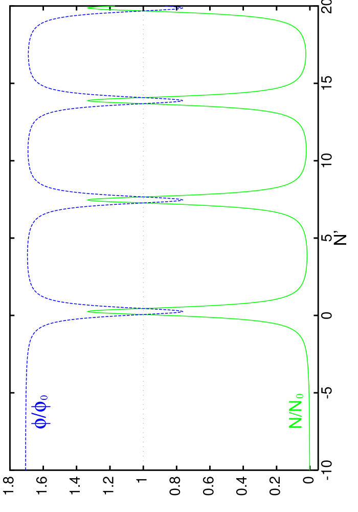
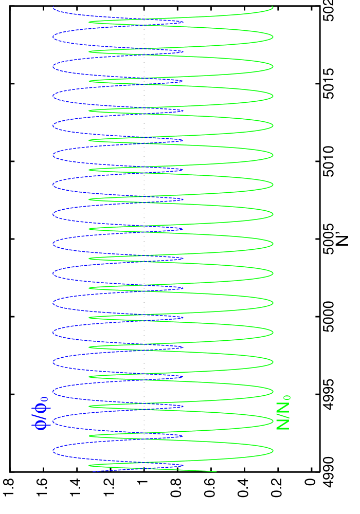
In Ref. [8] they have studied standard hybrid inflation with and found chaotic behaviour of the classical fields initially, that eventually becomes more regular. However, the SUGRA hybrid inflation model would correspond to , where the chaotic motion is not present and the trajectory is given by a straight line. This can be seen in Fig. (1), where we have plotted the oscillations of the classical fields and the trajectory in the plane, for the choice of parameters: , and , which correspond to the choice . We have also included for comparison the standard hybrid model with , and the same values of and . In both situations, the results will remain qualitatively the same when changing the value of , and accordingly those of and ; the main effect of reducing (increasing) the scale being a weaker (stronger) effect of the expansion of the Universe during the first oscillations.
 |
 |
 |
 |
Using the relation Eq. (24), we can effectively replace the two oscillating fields problem by a single field, for example , oscillating along the potential,
| (25) |
Near the origin the potential is almost flat, with the curvature becoming first negative and then changing sign and increasing as we approach and pass the minimum. Therefore, the field will tend to spend most of its time near the initial values, mainly varying when it approaches the minimum and the evolution speeds up. In a non-expanding Universe, and taking as initial conditions the asymptotic limit , the exact solution of the classical evolution equation is given by:
| (26) | |||||
where is defined when reaches the peak of the oscillation . In fact the motion can be decomposed into two different parts, which we label region I/II respectively:
Region I: when the field is near the minimum , the motion is more harmonic and the sine squared term in the right hand side of Eq. (26) can be neglected, i.e.,
| (27) |
Region II: when the field increases/decreases as .
In an expanding Universe, the main effect of the friction term in the evolution equation will be to reduce the amplitude of the successive oscillations (and thus the period), such that the amplitude will now decrease as the inverse of time. Then, we can approximate the behaviour of the field around each peak of the oscillations (region I) by,
| (28) |
where now . The actual decrease in amplitude over an oscillation period will depend on the ratio . However, during the first stages of the oscillations the dominant effect will be to render the total oscillation more harmonic (symmetric) around the minimum, more than to reduce the factor .
3.2 Particle production: , .
Due to the behaviour of the classical fields, we may expect particle production through parametric resonance when the field is around the peaks, that is, in region I when . Therefore, in that interval of time we can use the approximation given in Eq. (28) in order to convert the evolution equations for the quantum fluctuations, Eq. (5), into a Mathieu-like equation. Here we will be mainly concerned about the production of and particles, which indeed will occur in any SUSY model of hybrid inflation. Production of other species of particle will be model dependent, depending on how they couple to the classical fields.
We first analyse the equations neglecting the mixing terms, in Eq. (5). As before, we will use the fact that and follow a straight line trajectory, and work only with the classical field . The effective masses for the quantum fluctuations and are then given by:
| (29) | |||||
| (30) |
which, when the classical fields are near the minimum, become:
| (31) | |||||
| (32) |
We have kept only the contribution linear in the cosine and neglected the sub-dominant cosine squared contributions. Substituting these expressions into Eq. (7), and defining:
| (33) |
it is straightforward to get the parameters and entering in the Mathieu equation, that is,
| (34) | |||||
| (35) |
We notice that these parameters are functions of time, as is the case in models studied in an expanding Universe. The time dependence purely due to the expansion appears in the scale factor, , such that the momentum k is red-shifted as the system evolves, and in the damping of the amplitude of the classical oscillations, , which will cause to decrease appreciably in a Hubble time. On top of this, we have an extra time dependence related to the nature of the oscillations, which enters in the factor , and which would be present even in Minkowski space.
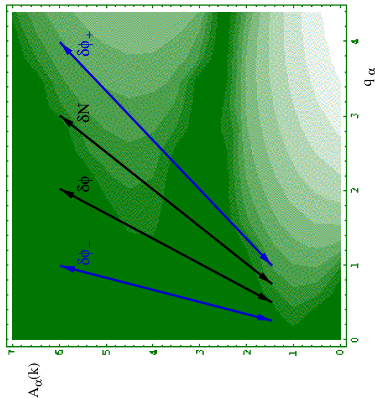
Although the Mathieu parameters and depend on time we can infer the behaviour of the solutions using the stability/instability bands analysis of the canonical Mathieu equation, (12). For a given mode k, instead of looking to a given point in the chart, we will move along some trajectory in the plane [4, 17], crossing different stability/instability regions as the fields oscillate. As long as we know the trajectory followed in the Mathieu chart, the standard analysis can be applied. For example, the parameters are bounded by,
| (36) | |||||
so that in each oscillation we will move in the Mathieu plot downward from right to left during the first half period, and back again. This can be seen in Fig. (2).
We first notice that for small values of the momentum k and , we have that but . The line roughly separates the broad (to the right of this line in the Mathieu plot) from the narrow (to the left) resonance regimes, and accordingly we expect much less production of particles than particles. To see the difference between broad/narrow regimes, we can follow Ref. [4] in order to get the maximum growth index in a trajectory of the type , with being the momentum. This is given by,
| (37) |
with:,
| (38) |
The value should be understood as an upper bound on the effective growth index along the given trajectory. Along the line (i.e. ) we have a constant maximum possible growth index, [2, 4]. Because we are crossing several stability/instability bands in only half a period, it has been argued than the effective will somehow be less than half this value, with the exact value depending on the actual time dependence of the parameters, and how much time is spent in each band. To the left of this trajectory, , we have that grows with and then decreases as we move from left to right in the Mathieu plot. In the opposite case, , we have the reverse behaviour with increasing with large , and we are in the broad resonance regime.

Then, it is clear that production is in the border line between the broad and narrow resonance, and the resonance can be quite efficient in producing them. With respect to production, we only get a non negligible value of in a small part of the trajectory, as can be seen in Figs. (2) and (3). Given the constraints in Eq. (3.2), at the beginning production occurs in the second resonance band, whilst may partially enter the first resonance band (see Fig. (3)). Moreover, even if the motion is not very suppressed by the Hubble expansion, parametric resonance takes place only during a fraction of the total period of the motion, so the final effective parameter averaging over several oscillations will be much smaller. Hence, for the particles we expect a narrow resonance if at all for momenta . As the damping factor gets reduced in time, production will be shifted further to the left in the Mathieu chart, into the narrow resonance regime.
However, particles with low momenta may be produced when the classical fields are not near the minimum, although this has nothing to do with parametric resonance. Whenever the effective squared mass of the field, Eq. (30), becomes negative and we enter the spinodal instability region. In this region, for the modes for which , we will again have an exponential increasing solution that can be interpreted as production of particles. At the end of the day, it seems that production of particles is quite efficient for modes with , and extremely effective for small modes below roughly .
So far, so good. These would be the qualitative results if the , , were negligible, but this is never the case in SUSY hybrid inflation. The analysis with the mixing term for the , system is greatly simplified given the fact that the background fields follow a straight line trajectory, implying only one oscillating mode. Hence, the coupled system for their quantum fluctuations can also be decomposed into two orthogonal modes,
with . The time dependent frequencies for the modes are now given by:
| (39) | |||||
| (40) |
and the corresponding parameters in the Mathieu equation are:
| (41) | |||||
| (42) |
The Mathieu parameters for the mode appear well to the left of the line , i.e. deep in the narrow resonance regime (see Fig. (2). However, for the mode we have the reverse situation, and the amplification of this mode will occur in the efficient broad resonance regime. Moreover, the effective mass becomes negative when , and again we will also have production of particles in region II of the classical oscillation.
Finally, given that , both and are dominated by the production in the mode,
| (43) |
leading to roughly the same rate of production for both particles. Moreover, in this case the mixing enhances the rate of production of particles compared with what was expected without it. This enhancement is a two-fold effect: on one hand parametric resonance is more effective due to the mixing, on the other hand we have a greater negative frequency in region II, with , which will imply a wider range of momenta, , in which particles can be more efficiently produced.
To illustrate these points, we have numerically integrated the equations with , and , and obtained the occupation number of particles, Eq. (10). The results are plotted in Fig. (4), and we have included for comparison those obtained when neglecting the mixing (left plot). Without the mixing, particles are hardly produced, whilst production of particles with low momenta proceeds quite quickly. Moreover, we can distinguish clearly in the plots the two different mechanisms of particle production. The peaks in are due to parametric resonance in an expanding Universe, whereas between peaks grows almost linearly in the first few oscillations reflecting the presence of a negative squared frequency in the evolution equation for these modes. When the Hubble expansion has reduced the amplitude of the oscillation such that (without mixing) or further to (with mixing), the occupation numbers become constant between the peaks. When the mixing is included (right plot), the occupation numbers for both particles become comparable, and the rate of production of particles is enhanced compared to the situation without the mixing.
 |
 |
3.3 Comment on backreaction.
Up to now, the analysis of particle production in the SUSY hybrid model has been done neglecting backreaction effects. Even if no other particles couple to the inflaton and fields, it can be inferred from Fig. (4) that the production of their own quanta will soon affect the evolution of the system. Due to the presence of the tachyonic mass immediately after the end of inflation, these fluctuations may grow and modify the classical evolution even before the fields reach the minimum for the first time. After the inflaton has crossed the critical value, the classical fields may still move in the slow-rolling regime for a while, and we can consider that the Universe continues inflating for a further fraction of an e-fold (for the parameters of Fig. (1) ). The first effect of the instabilities during this period would be to speed up the evolution and end the slow roll regime and thus inflation altogether. Their contributions to the classical equations can be computed using the Hartree Fock approximation111A brief description of this approximation is given later in section 4.3 and Appendix B. and can be interpreted as corrections to the effective masses of the fields. Thus, even in the slow roll regime with , the mass of the inflaton becomes,
| (44) |
When the fluctuations grow such that both terms become comparable, the inflaton (and by extension the field) is pushed away from the slow roll trajectory. These contributions are dominated by the modes with the lower values of the momentum k, but their evolution will tend to follow that of the background fields (for small enough values of k, the equations of motion are the same). As the classical fields reach the minimum and begin to oscillate, production of particles in these low momentum modes practically stops, and production begins in slightly higher modes. This effect is similar to the “zero mode assembly” described in Ref. [9] in the context of new inflation type models. Despite the differences, new inflation and hybrid inflation share the fact that both end with a phase transition. Under certain conditions, it is shown how the spinodal instabilities drive the growth of the quantum fluctuations such that they dominate completely the inflationary dynamics ending inflation. The super-horizon modes together with the inflaton follow the same evolution and assemble into an effective zero-mode field which drives the dynamics of the system. In hybrid inflation, the contribution due to the particles produced in the lower modes during the pre-oscillatory, quasi slow-rolling regime, speeds up the initial evolution towards the minimum, but it does not reach the level of modifying the oscillatory regime. For this to happen, we have to wait until higher modes have been populated and become dominant.
On the other hand, other particles can be present and these might be more efficiently produced during the oscillatory phase, such that they would dominate the backreaction effects. Given that in the original SUSY superpotential we have complex fields, their imaginary components, CP-odd singlet scalars, are among the particles that should also be included in the game. However, because the couplings to their real partners is model dependent, we will not attempt to study the production of these particles in a general way here. We will rather focus in the next section in a particular supersymmetric model of inflation motivated by particle physics considerations, where these questions can be addressed.
4 A particular model: NMSSM Hybrid Inflation
The NMSSM [18] is a simple modified version of a well known particle physics theory, the next-to-minimal supersymmetric model (NMSSM). As such it is a realistic working supersymmetric model which supports inflation. The model has been formulated in the context of a SUGRA theory in [16]. We will briefly review the global SUSY model here.
The model is based on the superpotential:
| (45) |
where are the standard Higgs doublet superfields, and N and are singlet superfields. As in the usual NMSSM, and are two dimensionless coupling constants. Since the singlet, is linear in the superpotential, the potential will be very flat in its direction enabling it to act as the slowly rolling inflation field.
This superpotential admits a global Peccei-Quinn symmetry which forbids further terms and solves the strong-CP problem. The symmetry is broken at the scale of the singlet VEVs giving rise to an invisible DFSZ axion of that scale. Whilst the axions may provide a Dark Matter candidate, they must be tightly constrained in order not to over close the Universe or destroy the results of nucleosynthesis. Axions may be produced directly during the explosive preheating phase or they may be a decay product of the other massive particles produced during preheating.
Previous to the start of inflation it is assumed that the field is driven to zero. During inflation the standard Higgs fields may be ignored and the scalar potential in terms of the canonically normalised real fields and , becomes:
| (46) |
The constant, has been added to ensure the necessary vanishing of the potential at its global minimum which corresponds to our vacuum and the critical values of for which the effective mass vanishes have been written explicitly in the potential and are given below in terms of the soft SUSY parameters, which appear in the soft SUSY-breaking part of the potential, ,
| (47) |
The first derivatives of the potential are,
| (48) |
Taking the fields to be positive, the (tree level) global minimum is found to be,
| (49) |
and thus the vacuum energy which must be zero at the global minimum is given by,
| (50) |
In the SUGRA model [16] is provided in the hidden sector by the moduli and dilaton contributions.
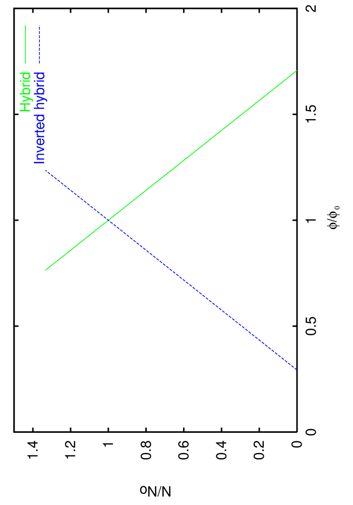
As usual, during inflation the field is trapped in its false vacuum, , whilst the field slowly rolls along the potential either from above towards the origin (hybrid) or from below and away from the origin (inverted hybrid [19]), depending on whether the small inflaton mass squared, , is positive or negative respectively. Once at the critical value, the mass changes sign and both singlets roll down towards the global minimum signaling the end of inflation.
The distinctive feature of having two critical values, , relies on the presence of the trilinear parameter in the potential. Since we expect in order to motivate the parameter of the MSSM, the inclusion in the potential of the SUSY-breaking soft parameters, masses and trilinears, is mandatory in our model. However, once the potential is written as in Eq. (46), it can be seen as a generalisation of the SUSY hybrid potential, independently of the origin of the mass parameters. In the limit ,(), and thus , we recover indeed the standard SUSY hybrid potential,
| (51) |
Therefore, the main difference between Eqs. (46) and (51) lies in the origin of the scale . In standard SUSY F-term hybrid inflation, this is given in terms of an intermediate mass scale coming directly from the superpotential, Eq. (15), whereas in our model no explicit mass scale is included in the superpotential and the critical value, , is generated via soft SUSY-breaking. From the cosmological point of view, this in turn will mark the difference between the models through the value of the Hubble constant and the vacuum energy during inflation.
Whatever the origin of the critical scale , the parameters in the model must satisfy the COBE constraints and the slow rolling conditions, Eqs. (16-19). Since in our model must not exceed the bound on the axion scale, and moreover , rough order of magnitude estimates for the parameters in the potential are found to be: , hence the vacuum energy and Hubble constant are small, , . Note that terms involving the Higgs doublets in the potential, (see Appendix A, Eq. (A)), will be at least a factor below the value of above so essentially these fields will not contribute at all towards the vacuum energy. We result with a scale independent spectrum, predicted to an accuracy of . The inflaton mass, comes from radiative corrections to its zero tree-level mass. The smallness of and , the origin of and the massless tree-level inflaton can be explained in terms of a no-scale SUGRA, superstring inspired theory in [16] where it is also shown that the -problem common to most (-term) inflation models can be avoided here.
In the next subsections we give the results of our investigation of the post-inflationary stage of the NMSSM model described in the previous section. Firstly we analyse the behaviour of the classical homogeneous background fields according to the classical potential, neglecting particle production (Figs. 5-7); secondly we study the quantum fluctuations on the classical background of all fields in the theory, relating the growth of these fluctuations to particle production (Figs. 8-10); and lastly we find an estimate of the point at which backreaction of created particles becomes important and show the immediate effect this has on the classical field evolution (Figs. 12-14).
Within the approximate order of magnitude results necessary to realise the model, we have chosen the set of parameters below for our numerical study:
| (52) | |||||
More explicit details and calculations involving the other fields in the potential needed in the analysis of the post-inflation era are given in the Appendix at the end of the paper.
4.1 Classical results - neglecting particle production
Being no more than a particular version of the SUSY F-term hybrid model, the NMSSM model leads to an evolution of the classical homogeneous fields, and (ignoring particle production) which follows the general pattern given in section 3.1. In this case the inflaton field will oscillate around its non-zero VEV, . The two ratios of scales that fix the behaviour of the oscillations are:
(a) ; the motion begins with extremely small slow-rolling values, and moreover the contribution of the tiny inflaton mass becomes negligible very soon in the evolution. As a result, the fields will follow the straight line trajectory (Fig. (5) to a very good degree of accuracy, and the actual oscillations of the fields are indeed in phase.
(b) ; the oscillations will begin with very large, lightly damped amplitudes, and oscillate times in a Hubble time.
Fig. (6) shows the evolution of the fields from the moment the critical point is passed. The time scale displayed is in terms of the approximate number of oscillations of the fields, given by:
| (53) |
where one e-fold () corresponds to roughly oscillation times. This approximation becomes more exact as the oscillations approach simple harmonic motion at late times in the evolution when the amplitudes are very small and the masses given by (69) become a better approximation to the actual frequency of these late oscillations. In several of the plots we have used the variable , where is defined to be the moment when the fields reach the global minimum for the first time.
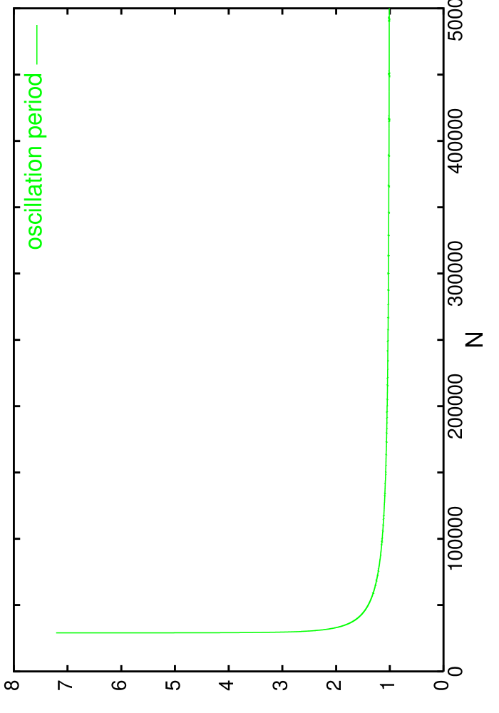
We can see in Fig. 6 that the fields take a reasonable length of time, oscillation times (about 1/10 of a Hubble time) before they begin to oscillate, so in fact inflation continues for just a fraction of an e-fold after the critical point is passed. The fields then begin to oscillate with amplitudes decreasing due to the expansion of the Universe. In terms of a Hubble time, the total amplitude will decrease rapidly at first and more slowly as time progresses until after about 2 e-folds the oscillations have decreased to th their original amplitude. The frequency of oscillations increases as they progress, and the motion eventually evolves towards simple harmonic. The period of oscillation rapidly decreases to begin with, indicating that in comparison to the Hubble time, simple harmonic motion becomes a good approximation relatively early on in the stages of oscillation. However, particle production will occur during the first few oscillations which are far from harmonic.
Due to the low value of the Hubble constant relative to and hence the little effect it has on the amplitude of the first oscillations, in the top right panel in Fig. (6) we can clearly distinguish the two different parts of each oscillation: the peak, corresponding to more harmonic-like motion around the minimum, Eq. (28), and the non-oscillating section where the fields decay as as they approach the initial values. This second part of the motion is rapidly affected by the expansion of the Universe as it causes a slight decrease in the amplitude, and at later stages (top right) it is further suppressed.
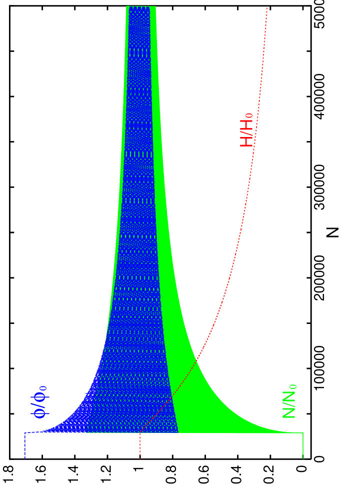
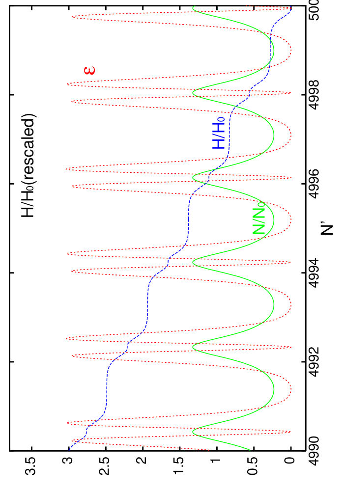
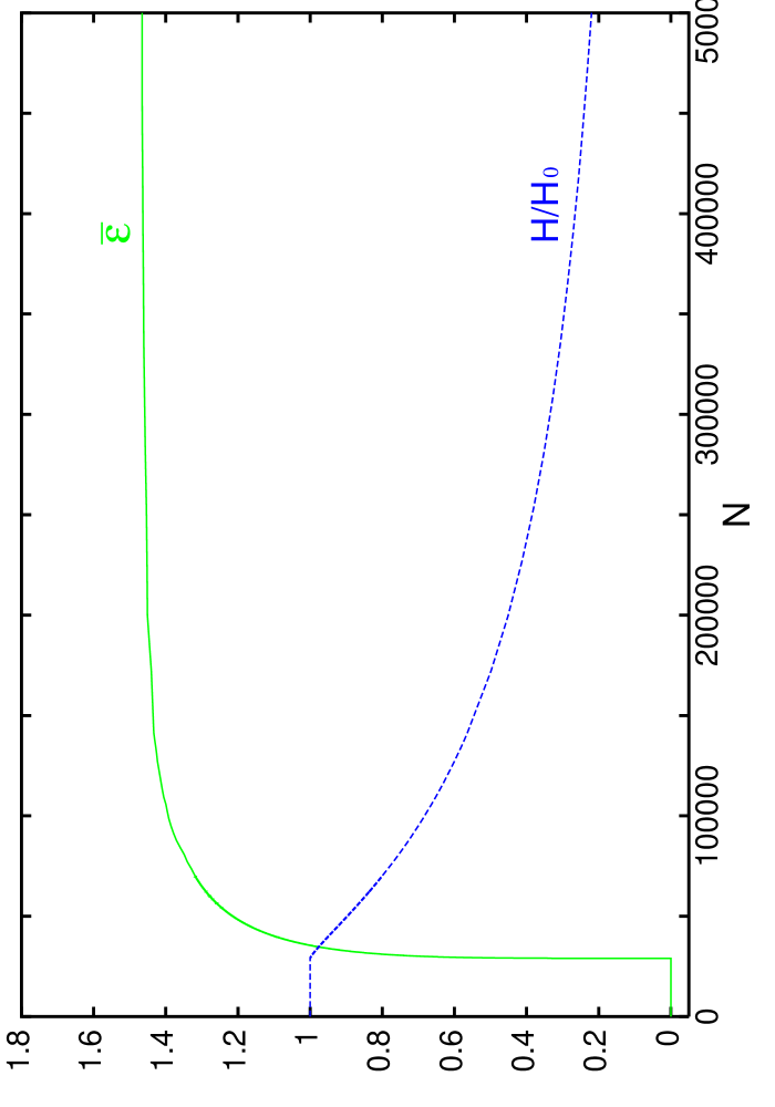
The behaviour of the Hubble constant is shown in Fig. 7 where we have also plotted the quantity . corresponds to the vacuum dominated era of inflation, to the reheating phase when matter (specifically the decay products before they have thermalised) dominates, and to the final (after the reheat temperature has been reached) radiation dominated Universe. During the oscillations, oscillates between the values 0 and 3 and its average value per oscillation, shows the transition between vacuum and matter dominated states.
4.2 Quantum effects - Preheating
Treating as fluctuations in the presence of the background fields, which have the independent dynamics described in the previous section, we solve the equations of motion for the quantum fluctuations of all scalar fields in the theory,
| (54) |
where . Here, the term in Eq. (7) is negligible since the Hubble constant is so small relative to and (see Fig. (7)) so is also small in this model. In fact, particle production will take place in a tiny fraction of a Hubble time, and we can safely neglect any effect due to the expansion of the Universe in the following. Since we are not considering the quantum fluctuations of the standard Higgs fields, , (see Appendix A), the system above reduces to two sets of two coupled equations describing the quantum fluctuations of the , , the axion and fields. The axion and the field are the massless/massive pseudoscalars in the model, defined in terms of the imaginary components of the complex fields,
| (55) |
with . The mass squared matrices, , are given in Eqs. (68) and (73) in Appendix A.
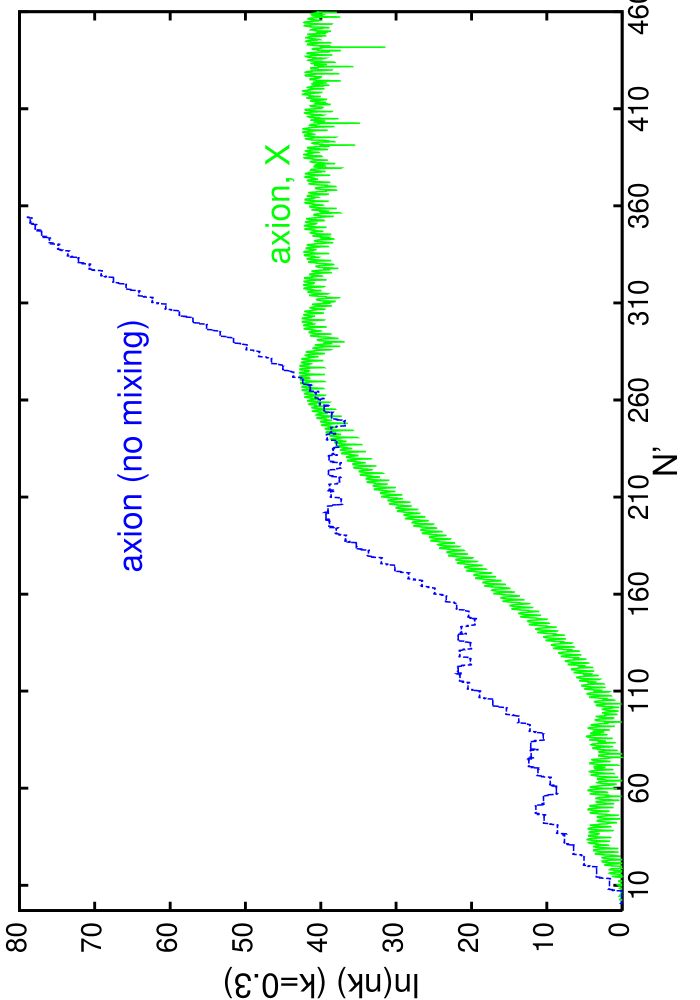
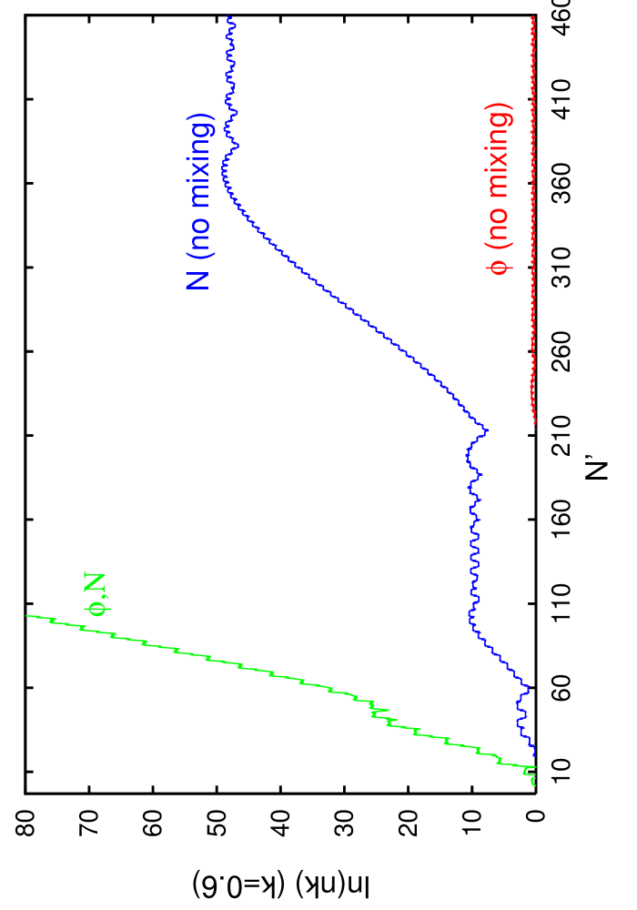
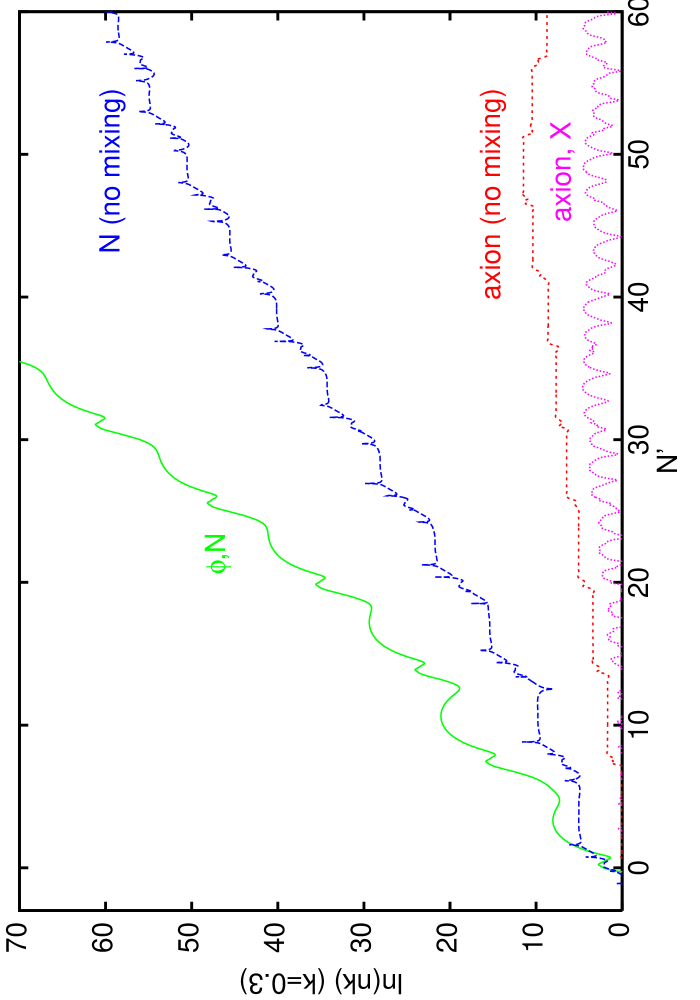
The results obtained by solving the equations numerically for the parameters given in (52) are summarised in Figs. (8-10) where the occupation number is defined in Eq. (10). In fact particle production appears to be extremely efficient.
We have also plotted for comparison the results obtained treating each particle separately and solving Eqs. (54) as if they were four uncoupled equations, ie. without the mixing terms () in the mass squared matrix . In particular in Fig. (8) we can see that with mixing there are less axions produced, but now s are also produced at the same rate, whereas particle production increases considerably and now particles are also produced at the same rate. The numerical results for the system fit quite well with the analytical behaviour obtained in section 3.2 using the Mathieu equation .
In the axion- system, the analysis based on the Mathieu equation will depend on the details of the model, for instance the value of , and some of the approximations may not be valid, such as neglecting terms proportional to the cosine squared in the effective masses. Bearing this in mind, we still can get some qualitative features studying the equations without the mixing term. The Mathieu parameters are then given by:
| (56) | |||||
| (57) | |||||
| (58) | |||||
| (59) |
where the RHS numerical factors correspond to . We notice that production of particles would be practically non-existent, whilst axions may be produced but with , which leaves us in the narrow resonance regime. However, these are only indications of what could happen if the axion and X were not coupled. Due to the mixing term, we get that both particles are produced at the same rate, but in this case the production of axions will be further suppressed.
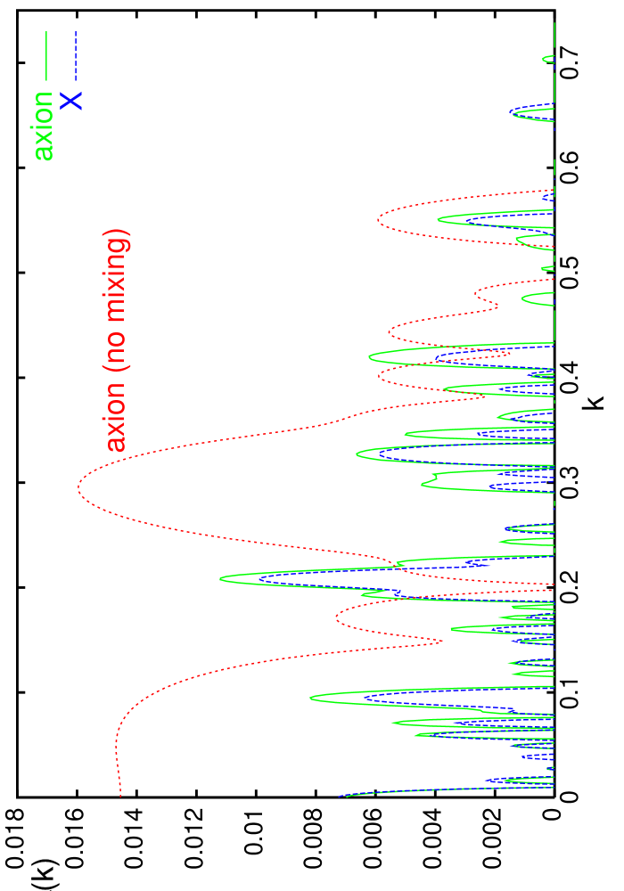
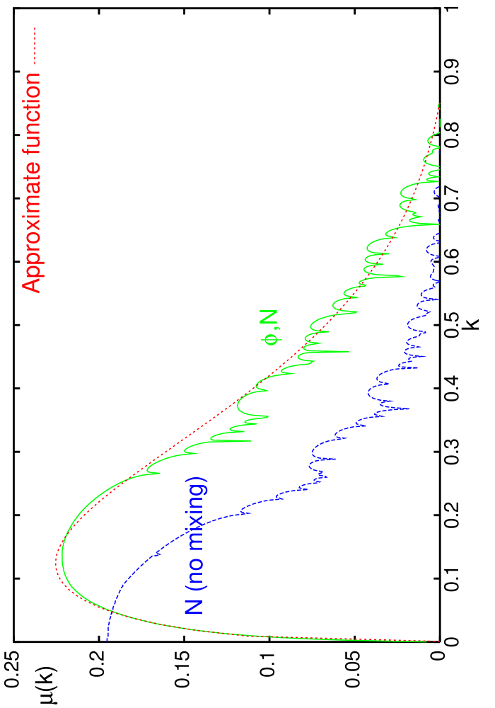
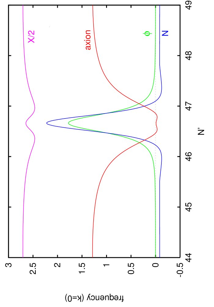
Fig. (9) plots an estimate of the initial rate of growth of the occupation number of each particle as a function of the wavenumber , Without taking into account the mixing terms, the largest rates correspond to the lowest mode, whilst with the mixing the effective growth index for and particles is negligible for , but it has a maximum around . As mentioned in section 3.3, the lower modes follow the evolution of the homogeneous fields and their production is suppressed during the oscillations. For a particular typical value of , Fig. (10) shows the relative rates of production of particles. For the beginning oscillations, the classical fields spend less than 1/6 of the total period of the oscillation around the minimum, where parametric resonance takes place. In Fig. (10), this would correspond to the spikes in the rate of production with no mixing. Thus, the relatively large values of for low values of the momentum is produced by a simpler mechanism, and is due to the presence of negative squared frequencies in the evolution equation of the quantum fluctuations, as can be seen in Fig. (11). On the other hand, we want to stress the fact that with mixing the rate of production for the axion and the are brought together, but this now corresponds to a smaller rate of production for the axion. We will see in the next section that indeed the total number of axions produced is several orders of magnitude smaller than that of the inflaton and particles.
The situation for the pseudoscalars may change depending on the model. For example, in models where , () there would be no mixing among the massive and the massless pseudoscalars and the axion would be the imaginary component of the field. When particle production begins, the effective squared mass for the axion would be given by (see Eq. (70) in Appendix A),
| (60) |
which again becomes negative whenever . In this case, we would find that indeed the production of axions may proceed at the same rate as that of the inflaton and particles in a extremely efficient way.
4.3 Effects of backreaction.
Due to the extremely large numbers of and particles produced during the first few oscillations of the background fields, these particles will quickly give a non-negligible contribution to the evolution equations. Therefore, instead of the tree-level equations considered until now, the full dynamics taking into account the interactions among the particles being produced should be included in the evolution equations. In practice this means that the polarization tensors for the different fields must be computed beyond the tree-level approximation. A consistent treatment of all non-linear effects involved can be obtained by using lattice techniques [5, 6]. However, in order to get some insight on how backreaction affects the process of preheating, the Hartree approximation [20, 21] for the potential should be good enough.
Within the Hartree approximation, the main one-loop contributions to the tadpole and mass terms in the potential are included, not only for the background fields but for any quantum field. A summary of how to expand the potential and the new expressions for the effective masses are given in Appendix B. Including one-loop corrections, the effective mass of the fields pick up new non-thermal contributions proportional to,
| (61) |
For example, the effective mass for the inflaton field and its quantum fluctuation will become:
| (62) |
where is the mixing angle in the axion- sector defined in Appendix A. The average can be seen as a closed loop of a particle . The Hartree approximation does not cover all possible types of contributions to the polarization tensors, and the effects of rescattering among the different species are missed. However, by integrating the coupled system of equations together with Eq. (61), it succeeds in summing up the infinite set of diagrams of the “cactus” or “daisy” type. The overall effect of the change in the effective masses will be to shut down the explosive production of particles. On one hand, it will increase the frequency of the oscillation of the background fields, hence decreasing their amplitudes; on the other hand, it will render the squared frequencies of the quantum fluctuations positive, ending the process.
Using the results of the previous section we can estimate the time at which backreaction becomes important, that is, when . The expectation values are related to the total number of particles produced, and the later can be estimated given the growth index function . It is then clear from Fig. (6) that we have to worry mainly about and production, and that the total number of axions and fields is several orders of magnitude smaller. This simplifies life, because the function for the fields and can be quite nicely approximated by:
| (63) |
valid for the first few oscillations. The total number of particles (or ) produced at a time is then:
| (64) |
and we get when . Therefore, backreaction effects will become important just after the third oscillation of the inflaton field. Soon after that, the results given in the previous section are modified and quantum fluctuations cease to be produced at a exponential rate. As a consequence, we will never reach the point where we have produced too many axions (see Fig. (8)).
In Fig. (9) it can be seen that only particles with low momenta, , are effectively being produced. Then, the value can be used as a cut-off in the momentum integrals, especially when computing the expectation values . In principle, these quantities are quadratically divergent and have to be renormalised [22]. In practice, we avoid this subtle point using the cut-off; the rest of the couplings and mass parameters appearing in the equations are then taken to be the renormalised ones.

The numerical results confirm our estimation. In Fig. (12) it is shown how the oscillations for the background fields change after . However, they are still in phase and follow the trajectory given in Fig. (5). Recently, it has been stressed that, in models with symmetry breaking, backreaction of the quantum fields could restore the original symmetry [23], if they come to dominate the effective mass during the stage of preheating. This is not the case in our particular model. Backreaction itself prevents the quantum fluctuations from reaching the stage where they might restore the symmetry. However, the shape of the potential changes and when particle production has effectively stopped, the classical fields end oscillating around a minimum different to , . We stress that the whole preheating process takes place within much less than a Hubble time. This means the expansion of the Universe can be neglected during this time. The decrease in the amplitude of the oscillating fields in Fig. (12) is purely due to the presence of the fluctuations.

In Fig. (13) we give the rate of production for all the different species of particle with a typical momentum . Soon after they reach a plateau, signaling the near end of the preheating period. Fig. (14) shows the total number of particles per comoving volume being produced. We end with the ratio of scalars to pseudoscalars being ). Preheating is very efficient in producing and quanta, and in fact it is this effect which precludes other particles from being so efficiently produced. Backreaction due to and affects the evolution of field (classical and quantum) in the model.
This, however, may not be the end of the story. The Hartree approximation neglects the effects of rescattering among the particles produced, but it is possible that these terms could be the same order of magnitude as the expectation values [4]. Lattice simulations [6] for one-field inflation models have shown that the maximum value of is overestimated in the Hartree approximation when the resonance is very efficient. However, once this maximum value is reached the resonance ends qualitatively in the same way as in the Hartree approximation. It is difficult to extrapolate from these studies to our model. We may have overestimated the total number of and produced, and/or it may happen that rescattering may induce an extra little production of axions and . But it is unlikely this could reduce the large gap among and . We can venture that, after preheating, the Universe will end with the classical fields still displaced from the global minimum, and fill up with nearly non-relativistic particles, a large fraction of them being and . A fraction of the energy storage in the inflaton field at the end of inflation has been transferred to the particles produced, and this will set the initial conditions for the subsequent evolution of the system, as given by the standard theory of reheating; in the Hartree approximation roughly 60% of the initial energy density is converted into quantum fluctuations. Moreover, by the time reheating is complete, any density of stable particles (i.e. axions) would be diluted by the entropy released in the decay of the and .

5 Conclusion
We have analysed in this paper the preheating era which occurs immediately after the end of inflation in a general SUSY model of hybrid inflation. From the point of view of the inflationary potential it is no more than a particular case of the general hybrid model, Eq. (13). Still, preheating in this particular model is found to be quite different when studied in more detail. Supersymmetry leads to equal masses at the global minimum for the real singlets relevant to inflation ( the inflaton and ), and therefore to the presence of a common frequency of oscillation for the classical fields. That is, the supersymmetric potential allows an approximate solution with only one mode of oscillation for the classical fields, the orthogonal one being stationary. This solution becomes exact as the explicit tiny mass of the inflaton, , tends to zero. Due to the inflationary dynamics (slow roll conditions) this mass is indeed always negligible, independently of the value of any other parameter. Moreover, the slow roll scenario also fixes the initial conditions at the beginning of the reheating era such that we begin with very small initial velocities. Therefore, the fields will follow almost exactly a straight line trajectory, oscillating with equal frequencies and proportional amplitudes. Hence, for the purpose of studying particle production, the SUSY hybrid model can be simplified to a single field model (the oscillating mode), with the potential given in Eq. (25).
Since we are dealing with an effective single field oscillating, we can attempt to convert the evolution equations for the quantum fluctuations into Mathieu-like equations, whose solutions in term of stability/instability regions is well known. We have first studied production of and particles, which is completely independent of the details of the model. Even in a first approximation neglecting the effects of backreaction, the evolution equations are coupled through mixing terms in the effective mass matrices. The equations for and taken independently (that is, neglecting the mixing term) result in a higher rate of production of particles than , the latter being almost completely suppressed. However, the effect of the mixing term is to bring together the rate of production for both particles, and overall to become more effective indeed. The fact that we achieve almost the same number of particles is general to any system of coupled particles with non negligible mixing. In other words, during the preheating proccess we can produce particles which in principle are not expected to exist, if they are coupled to other particle species which are efficiently produced. The rate of production of the latter will be increased/decreased depending on the strength of the mixing.
Given that hybrid inflation ends by a phase transition, for some values of the fields tachyonic masses will be present, for example that of the field. As well as an initial production of particles when the fields are first moving towards the minimum, if the amplitude of the oscillations is large enough there will be additional production of particles between oscillations when the classical fields are in the unstable region of the potential with negative curvature. Therefore, it is the combination of parametric resonance and tachyonic mass which causes the production of and particles to be so efficient.
Production of and fluctuations will rapidly give rise to non-negligible backreaction effects which will modify the subsequent evolution of the system. However, other particles may be efficiently produced in the model which can also contribute to this effect. With this issue being model dependent, we have proceeded to analyse the situation in a particle physics based model of inflation, the NMSSM [18]. This model is not only suitable for inflation, but also solves the strong CP problem by an approximate Peccei-Quinn symmetry and leads to an invisible axion, which could be dangerously produced during preheating. However, in this case the mixing term between the axion and the massive pseudoscalar slightly suppresses the axion production rate, which turns out to be much smaller than that of the real scalars. Nevertheless, we obtain the same general result of comparable rates of production for both pseudoscalars. Backreaction effects are then dominated by the production of the real components of the fields, which quite rapidly succeed in preventing the production of any other particle species. Therefore, axions in this model are kept safely under control, thoughtout and after the preheating era.
Acknowledgements
We thank Juan García-Bellido both for motivating this work and for discussions.
————————————————————————–
Appendix A Appendix
Here we present some further calculations on the NMSSM model, involving all scalar fields in the theory.
The superpotential,
leads us to the full Higgs part of the tree level scalar potential:
where is the usual -term of the MSSM. The full spectrum of scalar fields is listed below,
| (66) | |||||
with VEVs given by:
| (67) |
where the electroweak values, .
The full mass squared matrix for the scalar fields is defined by, , where is taken to mean each of the real and imaginary fields in (66). When the standard Higgs are at their VEVs, consists of two lots of matrices for the CP-even and CP-odd neutral sectors, and two standard MSSM blocks for the charged mass matrices. All other entries are zero since the charged sectors do not mix with the neutral ones and the CP-odd and -even sectors do not mix.
In fact the matrices can be further split into two matrices since mixing between the singlets and the standard neutral Higgs (at least when taken at the VEVs) are suppressed at the very least by a factor with respect to the other terms, so can be neglected. (Note that in general though, these terms may be non-negligible and then must be included in Eqs. (5), leading to the possibility of parametric production of Higgs particles and also a change in the production rates of other particles.) We are then left with standard MSSM matrices for the CP-even neutral Higgs and also for the CP-odd sector with the usual massless mode and mixing angle given by, . The mass squared matrix for the real singlet fields is given by,
| (68) |
where and denote the real classical fields, the imaginary parts of which are held at zero. Again, here terms due to coupling to the standard Higgs are very suppressed with respect to the other terms so have been neglected.
At the global minimum, (68) is diagonal with the masses equal,
| (69) |
where the bar is used to stress that the masses are at the global minimum.
Similarly the CP-odd mass squared matrix for the pseudoscalar singlet fields, and is:
| (70) |
As in the CP-even matrix (68), we have neglected the small couplings to the standard Higgs. Diagonalising when the fields are at their VEVs gives us the massless mode (axion, ) , and the massive pseudoscalar, , , with mixing angle, given by,
| (71) |
with the axion and it’s massive counterpart defined in terms of the imaginary components, , by:
| (72) |
The mass squared matrix, in the basis , then becomes,
| (73) |
where,
Appendix B Appendix
With particle production in mind, we now proceed to obtain the equation of motion in the Hartree approximation. Written explicitly in terms of the four fields, , , and , the full potential, (46) becomes:
| (74) | |||||
where,
and and are as given in Appendix A above with replaced now by , . The fields are decomposed as in Eq. (1), and the potential is expanded assuming the factorization:
| (75) |
Each term in the factorization can be seen as the contribution from a one-loop diagram, with the contractions accounting for the internal propagator in the loop; only those terms which correspond to physically allowed diagrams are included in the expansion. In this way, one-loop contributions to the tadpole and masses are included, such that we end with a potential quadratic in the quantum fluctuations. Using this potential and the tadpole constraint we obtain the equations of motion as given in Eq. (2) and Eq. (5). The first derivatives , including the additional terms, are now given by:
| (76) | |||||
| (77) | |||||
with and as given in Eqs. (48), and we have defined,
In addition, the Friedmann equation for a Universe containing classical fields and particles now reads:
| (80) |
with being the energy density of the different particles produced, i.e.,
| (81) |
References
- [1] E.W. Kolb and M.S. Turner, The Early Universe, Addison-Wesley, Redwood City, CA 1990.
- [2] L. A. Kofman, A. D. Linde and A. A. Starobinsky, Phys. Rev. Lett. 73 (1994) 3195.
- [3] A.D. Dolgov and A.D. Linde, Phys. Lett. B 116 (1982) 329; L.F. Abbott, E. Fahri and M. Wise, Phys Lett. B 117 (1982) 29.
- [4] Lev Kofman, Andrei Linde, Alexei Starobinsky, Phys. Rev. D 56 (1997) 3258.
- [5] S. Yu. Khlebnikov, I. I. Tkachev, Phys. Rev. Lett. 77 (1996) 219; T. Prokopec and T. G. Roos, Phys. Rev. D 55 (1997) 3768.
- [6] S. Yu. Khlebnikov, I. I. Tkachev, Phys. Rev. Lett. 79 (1997) 1607.
- [7] A. D. Linde, Phys. Lett. B 249 (1990) 18; A. D. Linde, Phys. Lett. B 259 (1991) 38; E. J. Copeland, A. R. Liddle, D. H. Lyth, E. D. Stewart and D. Wands, Phys. Rev. D 49 (1994) 6410.
- [8] Juan García-Bellido, Andrei Linde, Phys.Rev. D 57 (1998) 6075.
- [9] D. Boyanovsky, D. Cormier, H. J. de Vega, R. Holman, S. P. Kumar, Phys. Rev. D 57 (1998) 2166; hep-ph/9801453.
- [10] D. Boyanovsky, H. J. de Vega and R. Holman, Phys. Rev. D 49 (1994) 2769; D. I. Kaiser, Phys. Rev. D 57 (1998) 702.
- [11] N. W. MacLachlan, Theory and Application of Mathieu Functions, Dover, New York, 1964.
- [12] A. R. Liddle and D. H. Lyth, Phys. Rep. 231 (1993) 1.
- [13] E. F. Bunn, D. Scott and M. White, Ap. J 441 (1995) L9; E. F. Bunn and M. White, Ap. J 480 (1997) 6.
- [14] D. H. Lyth and A. Riotto, hep-ph/9807278.
- [15] E. Halyo, Phys. Lett. B 387 (1996),43; P. Binétruy and G. Dvali, Phys. Lett. B 388 (1996) 241. For earlier work on this subject see: J. A. Casas and C. Muñoz, Phys. Lett. B 216 (1989),37; J. A. Casas, J. Moreno, C. Muñoz and M. Quiros, Nucl. Phys. B328 (1989) 272.
- [16] M. Bastero-Gil, S.F. King, hep-ph/9806477, to appear in Nucl. Phys. B.
- [17] S. Yu. Khlebnikov, I. I Tkachev, Phys. Lett. B 390 (1997) 80; B. R. Greene, T. Procopec, and T. G. Roos, Phys. Rev. D 56 (1997) 6484; I. Zlatev, G. Huey, P. J. Steinhardt, Phys. Rev. D 57 (1998) 2152.
- [18] M. Bastero-Gil, S.F. King, Phys. Lett. B 423 (1998) 27.
- [19] D. H. Lyth and E. D. Stewart, Phys. Rev. D 54 (1996) 7186; Phys. Lett. B 387 (1996) 43; S. F. King and J. Sanderson, Phys.Lett. B 412 (1997) 19.
- [20] L. Dolan and R. Jackiw, Phys. Rev. D9 (1974) 3320.
- [21] D. Boyanovsky, H. J. de Vega, R. Holman, D. -S. Lee and A. Sing, Phys. Rev. D51 (1995) 4419.
- [22] See for example: D. Boyanovsky, D. Cormier, H. J. de Vega, R. Holman, A. Singh and M. Srednicki, Phys. Rev. D56 (1997) 1939.
- [23] L. Kofman, A. Linde and A. A. Starobinsky, Phys. Rev. Lett. 76 (1996) 1011; I. I. Tkachev, Phys. Lett. B 376 (1996) 35; A. Riotto and I. I. Tkachev, Phys. Lett. B 385 (1996) 57; G. W. Anderson, A. Linde and A. Riotto, Phys. Rev. Lett. 77 (1996) 3716; S. Kasuya and M. Kawasaki, Phys. Rev. D 58 (1998); S. Khlebnikov, L. Kofman, A. Linde and I. Tkachev, Phys. Rev. Lett. 81 (1998) 2012; M. Parry and A. Sornberger, hep-ph/9805211.