TAUP 2573/99

Total ${\mathbf{\gamma}^{*}p}$ Cross Section

E.  G O T S M A N¹⁾,        E.  L E V I N²⁾,

U.  M A O R³⁾    and    E.  N A F T A L I⁴⁾

School of Physics and Astronomy
Raymond and Beverly Sackler Faculty of Exact Science
Tel Aviv University, Tel Aviv, 69978, ISRAEL

Abstract:

This paper shows that the approach based on Gribov’s ideas for the photon-proton interaction, is able to describe the experimental data over a wide range of photon virtualities $Q^{2}=0-100\,GeV^{2}$ and energies $\sqrt{s}=W=3-300\,GeV$. A simple model is suggested which provides a quantitative way of describing the matching between short and long distances ( between “soft” and “hard” processes ) in photon-proton interaction at high energy. The main results of our analysis are: (i) the values of the separation parameters differentiating the “soft” and “hard” interactions are determined; (ii) the additive quark model can be used to calculate the “soft” contribution to the photon - proton interaction; (iii) a good description of the ratio $\sigma_{L}/\sigma_{T}$ is obtained ; and (iv) a considerable contribution of the “soft” process at large $Q^{2}$, and of “hard” processes at small $Q^{2}$ was found.

1 Introduction

The rich and high precision data on deep inelastic $ep$ scattering at HERA [1] [2], covering both low and high $Q^{2}$ regions, lead to a theoretical problem of matching the non-perturbative (“soft”) and perturbative (“hard ”) QCD domains. This challenging problem has been under close investigation over the past two decades, starting from the pioneering paper of Gribov [3] ( see also [4] ).

Based on Gribov’s general approach, one can interpret two time sequence of the $\gamma^{*}p$ interaction (see Fig. 1):

1. First the $\gamma^{*}$ fluctuates into a hadron system (quark-antiquark pair to the lowest order) well before the interaction with the target;

2. Then the converted quark-antiquark pair (or hadron system) interacts with the target.

These two stages are expressed explicitly in the double dispersion relation suggested in Ref. [3]:

$$\sigma(\gamma^{*}N)=\frac{\alpha_{em}}{3\pi}\int\frac{\Gamma(M^{2})dM^{2}}{(Q^{2}+M^{2})}\sigma(M^{2},M^{\prime 2},s)\frac{\Gamma(M^{\prime 2})dM^{\prime 2}}{(Q^{2}+M^{\prime 2})},$$ (1)

where $M$ and $M^{\prime}$ are the invariant masses of the incoming and outgoing quark-antiquark pairs, $\sigma(M^{2},M^{\prime 2},s)$ is the cross section of a $q\bar{q}$ interaction with the target, and the vertices $\Gamma^{2}(M^{2})$ and $\Gamma^{2}(M^{\prime 2})$ are given by $\Gamma^{2}(M^{2})=R(M^{2})$, where $R(M^{2})$ is the ratio:

$$R(M^{2})=\frac{\sigma(e^{+}e^{-}\rightarrow\mbox{hadrons})}{\sigma(e^{+}e^{-}\rightarrow\mu^{+}\mu^{-})},$$ (2)

which has beem measured experimentally. For large masses ($M,\,M^{\prime}>>M_{0}$) we have $\,\Gamma(M^{2}\,\geq\,M^{2}_{0})\times\Gamma(M^{\prime 2}\,\geq\,M^{2}_{0})\,\,\longrightarrow\,\,R(M^{2}\,\geq\,\,M^{2}_{0})\,=\,2$, where we assume that that the number of colours $N_{c}=3$. $M_{0}$ is a typical mass (a separation parameter), which is of the order of $M_{0}=1GeV$, determined directly from the experimental data [5].

Figure 1: The generalized Gribov’s formula.

The key problem in all approaches utilizing Eq. (1) is the description of the cross section $\sigma(M^{2},M^{\prime 2},s)$. In this paper we follow the approach suggested in Ref. [6], which is based on the ideas of Badelek and Kwiecinski [7]. Below we list the mains steps of this approach.

1. We introduce $M_{0}\,\,\approx\,\,1\,GeV$ in the integrals over $M$ and $M^{\prime}$ which plays the role of a separation parameter. For $M,\,M^{\prime}\,>\,M_{0}$ the quark - antiquark pair are produced at short distances ( $r_{\perp}\,\,\propto\,\frac{1}{M}\,\,<\,\,\frac{1}{M_{0}}$ ), while for $M,\,M^{\prime}\,<\,M_{0}$ the distance between quark and antiquark is too long ($r_{\perp}\,\,\propto\,\frac{1}{M}\,\,>\,\,\frac{1}{M_{0}}$), and we cannot treat this $q\bar{q}$ - pair in pQCD. Actually, we cannot even describe the produced hadron state as a $q\bar{q}$ - pair;

2. For $M,\,M^{\prime}\,<\,M_{0}$ we use the Additive Quark Model [8] in which

   $$\sigma(M^{2},M^{\prime 2},s) = \sigma^{soft}_{N}(M^{2},s)\,\delta(M^{2}\,-\,M^{\prime 2})$$ (3)

   $$= \left(\,\sigma_{tot}(qN)\,+\,\sigma_{tot}(\bar{q}N)\,\right)\,\delta(M^{2}\,-\,M^{\prime 2})$$

   The above assumption allows us to simplify the Gribov formula of Eq. (1):

   $$\sigma(\gamma^{*}N)=\frac{\alpha_{em}}{3\pi}\int\frac{R(M^{2})M^{2}dM^{2}}{\left(Q^{2}+M^{2}\right)^{2}}\sigma_{N}(M^{2},s)\,\,;$$ (4)

3. For $M,\,M^{\prime}\,>\,M_{0}$ we consider the system with mass $M$ and/or $M^{\prime}$ as a short distance quark - antiquark pair, and describe its interaction with the target in pQCD (see Fig. 2).

   The exact formulae for $\sigma^{hard}(M^{2},M^{\prime 2},s)$ is given below (see also Ref. [6]), but one can see from Fig. 2, that this interaction can be expressed through the gluon structure function, and it is not diagonal with respect to the masses, contrary to the “soft” interaction of a hadron system with small mass.

4. In principle, the short distance between the quark and antiquark leads to short distances in the gluon-nucleon interaction. However, the typical distance of the gluon interaction $r_{G}\,\,\propto\,1/l_{\perp}$ (see Figs 1 and 2) is larger than the size of the quark - antiquark pair and $l_{\perp}\,\,<\,\,{k_{\perp}}$. It turns out that the calculation with $M_{0}\,\,\sim\,\,1\,GeV$, demands a new scale in the gluon-nucleon interaction. We introduce it, assuming that the gluon structure function $xG(x,l^{2}_{\perp})$ behaves as $xG(x,\mu^{2})\,\times\,\frac{l^{2}_{\perp}}{\mu^{2}}$ for $l^{2}_{\perp}\,\leq\,\mu^{2}$. This means that we assume that the gluon-hadron total cross section is not equal to zero for long distances (in the “soft” kinematic region). It should be stressed that we introduce two scales for soft nonperturbative interactions, distinguishing between quark and gluon interactions. The two scales appear naturally in our models for “soft”, nonperturbative interaction. For example, in the AQM which we use for $\sigma^{\mbox{\scriptsize soft}}$, these two scales are the size of a hadron (distance between the quark and antiquark), and the size of the constituent quark which is related to gluon interaction scale.

5. As has been discussed, we use the AQM [see Eq. (3)] to calculate $\sigma^{\mbox{\scriptsize soft}}$. For the vector meson cross section the AQM leads to

   $$\sigma_{\mbox{\scriptsize R}}\,\,=\frac{1}{2}\left(\,\sigma(\pi^{+}p)\,\,+\,\,\sigma(\pi^{-}p)\right).$$ (5)

   For the pion-proton cross section, we use the Donnachie - Landshoff Reggeon parameterization [9], with an energy variable which is appropriate for the interaction of a hadronic system of mass $M$ with the target (see [6] for details).

   $$\sigma_{M^{2}N}(s)=A(\frac{1}{x_{M}})^{{\alpha_{{I\!\!P}}}(0)\,-\,1}\,\,+\,\,B\,\,(\frac{1}{x_{M}})^{{\alpha_{{I\!\!R}}}(0)\,-\,1},$$ (6)

   with

   $${\alpha_{{I\!\!P}}} = 1.079$$

   $${\alpha_{{I\!\!R}}} = 0.55$$

   $$x_{M} = \frac{M^{2}}{s}$$

   $$A = 13.1\,\mbox{mb}$$

   $$B = 41.08\,\mbox{mb}\,.$$ (7)

   The values of $A$ and $B$ are chosen so that (6) is valid for the $\rho$-proton interaction. Using (6) in Gribov formula (4) we derive the soft transverse contribution to $\sigma(\gamma^{*}p)$:

   $$\sigma^{\mbox{\scriptsize soft}}_{\mbox{\scriptsize T}}=\frac{\alpha_{em}}{3\pi}\int_{0}^{M_{0}^{2}}\frac{R(M^{2})M^{2}dM^{2}}{\left(Q^{2}+M^{2}\right)^{2}}\left\{A(\frac{1}{x_{M}})^{{\alpha_{{I\!\!P}}}(0)\,-\,1}\,\,+\,\,B\,\,(\frac{1}{x_{M}})^{{\alpha_{{I\!\!R}}}(0)\,-\,1}\right\}.$$ (8)

Figure 2: “Hard” contribution to $\sigma(M^{2},M^{\prime 2},s)$ in perturbative QCD .

It has been shown in [6] that even though the simple model discussed above reproduces the main features of the experimental data, it has several deficiencies which we wish to address:

• The calculations of the “soft” cross section appeared to overestimate the data, and to overcome this, the soft contribution was multiplied by a factor $\kappa=0.6$. There is no physical justification for such a small value.

• The contribution of a longitudinal polarized virtual photon to $\sigma(\gamma^{*}p)$ was neglected.

• An old GRV’94 parameterization was used for the gluons distribution inside the proton. This gave an energy dependence of $\sigma(\gamma^{*}p)$ which is steeper than the published data.

In the present paper we reexamine these points developing a formalism which also takes into account $\sigma_{\mbox{\scriptsize L}}$, the longitudinal part of $\sigma(\gamma^{*}p)$, for both the soft and the hard components. We find that the contribution of $\sigma_{\mbox{\scriptsize L}}$ significantly improves the energy dependence of $\sigma(\gamma^{*}p)$, in a good agreement with the data for $x<10^{-2}$.

A similar approach to photon - proton interaction was also developed in Ref.[10] where quite different scales have been introduced. The goal of such an approach (see Refs.[6],[7] and [10]) is to find parameters that separate the long distance (non-perturbative) and short distance (perturbative) interactions in QCD. A similar philosophy to ours is used in Ref.[11], where an attempt was made to describe photon - proton interactions, assuming that the main contribution stems from short distances, and the long distance interaction appears as a result of the shadowing corrections.

The description of $\sigma(\gamma^{*}p)$ can be achieved in quite a different way using the generalized vector dominance model[4] or a Regge motivated fit of the experimental data[12][13]. In these approaches one looses the explicit connection with the microscopic theory, which makes futher theoretical interpretation of the results rather difficult.

2 Description of the Model

2.1 The Contribution of a Transverse Polarized Photon

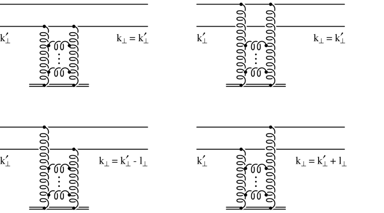
Figure 3: Diagrams which cntribute to the scattering of a $\bar{q}q$ pair off the target proton.

As we have discussed previously, the main assumption of our model is that $\sigma(M^{2},M^{\prime 2},s)$ in Eq. (1) can be calculated as

$$\sigma(M^{2},M^{\prime 2},s)=\sigma^{soft}_{N}(M^{2}\,<\,M^{2}_{0},s)\,\,\delta(M^{2}-M^{\prime 2})+\sigma^{hard}(M^{2}\,>\,M^{2}_{0},M^{\prime 2}\,>\,M^{2}_{0},s)\,\,.$$ (9)

In the previous section we have discussed the calculation of $\sigma^{\mbox{\scriptsize soft}}$. Now we present, for completeness, our formulae for $\sigma^{\mbox{\scriptsize hard}}$ which have been given in Ref. [6]. The pQCD contribution for $\sigma_{\mbox{\scriptsize T}}$, within the framework of the two gluon model, is illustrated in the four diagrams shown in Fig. 3. The production amplitude ${\cal M}_{{\lambda\lambda^{\prime}}}$ of the $\bar{q}q$, can be factorized into the wave function $\psi_{\lambda\lambda^{\prime}}$ of the $\bar{q}q$ system inside the virtual photon, and the amplitude ${\cal T}_{\lambda\lambda^{\prime}}$ for the scattering of the $\bar{q}q$ pair off the proton:

$${\cal M}_{\lambda\lambda^{\prime}}({k_{\perp}},z)=\sqrt{N_{c}}\int d^{2}{k_{\perp}}^{\prime}\int_{0}^{1}dz^{\prime}\psi_{\lambda\lambda^{\prime}}({k_{\perp}}^{\prime},z^{\prime}){\cal T}_{\lambda\lambda^{\prime}}({k_{\perp}}^{\prime},z^{\prime};{k_{\perp}},z)\,.$$ (10)

The transition ampiltude ${\cal T}_{\lambda\lambda^{\prime}}$ for the four contributions is:

$${\cal T}_{\lambda\lambda^{\prime}}({k_{\perp}}^{\prime},{k_{\perp}})=$$

$$i\frac{4\pi s}{2N_{c}}\int\frac{d^{2}\ell_{\perp}}{\ell_{\perp}^{4}}\biggl{[}2\delta(\mbox{\boldmath$k$}_{\perp}^{\prime}-\mbox{\boldmath$k$}_{\perp})-\delta(\mbox{\boldmath$k$}_{\perp}^{\prime}-\mbox{\boldmath$k$}_{\perp}-\mbox{\boldmath$\ell$}_{\perp})-\delta(\mbox{\boldmath$k$}_{\perp}^{\prime}-\mbox{\boldmath$k$}_{\perp}+\mbox{\boldmath$\ell$}_{\perp})\biggr{]}\alpha_{\rm S}(\ell^{2}_{\perp})f(x,\ell^{2}_{\perp})\,,$$

where,

$$f(x,\ell^{2})=\frac{\partial xG(x,\ell^{2})}{\partial\ln\ell^{2}}$$ (12)

(see [14] for details). Substituting (2.1) in (10) we have,

$${\cal M}_{\lambda\lambda^{\prime}}=i\frac{2\pi^{2}s}{\sqrt{N_{c}}}\int\frac{d\ell^{2}_{\perp}}{\ell_{\perp}^{4}}\alpha_{\rm S}(\ell^{2}_{\perp})f(x,\ell^{2}_{\perp})\Delta\psi_{\lambda\lambda^{\prime}}\,,$$ (13)

where the definition of $\Delta\psi$ is to be understood from  Eqs. (10)–(13):

$$\Delta\psi=2\psi(\mbox{\boldmath$k$}_{\perp},z)-\psi(\mbox{\boldmath$k$}_{\perp}-\mbox{\boldmath$\ell$}_{\perp},z)-\psi(\mbox{\boldmath$k$}_{\perp}+\mbox{\boldmath$\ell$}_{\perp},z)\,.$$ (14)

$\psi_{\lambda\lambda^{\prime}}$ has been calculated in [14] both for a transverse and for a longitudinal polarised incoming photon. The wave function for a transverse polarized photon and the amplitude for producing $\bar{q}q$ with helicities $\lambda$ and $\lambda^{\prime}$ read:

$$\psi^{\pm}_{\lambda\lambda^{\prime}}\left({\mathbf{{k_{\perp}}}},z\right) = -\delta_{\lambda,-\lambda^{\prime}}Z_{f}e\left[(1-2z)\lambda\mp 1\right]\frac{{2\mathbf{\epsilon}_{\pm}\cdot{k_{\perp}}}}{\bar{Q}^{2}+{k^{2}_{\perp}}},$$ (15)

$${\cal M}^{\pm}_{\lambda\lambda^{\prime}} = -2Z_{f}e\left(i\frac{2\pi^{2}s}{\sqrt{N_{c}}}\right)\delta_{\lambda,-\lambda^{\prime}}\left[(1-2z)\lambda\mp 1\right]{\mathbf{\epsilon}_{\pm}\cdot{k_{\perp}}}\int\frac{d\ell_{\perp}^{2}}{\ell_{\perp}^{4}}\alpha_{\rm S}(\ell_{\perp}^{2})f(x,\ell_{\perp}^{2})\,\times$$ (16)

$$\hskip 28.45274pt\left\{\frac{1}{\bar{Q}^{2}+{k_{\perp}}^{2}}-\frac{1}{2{k_{\perp}}^{2}}+\frac{\bar{Q}^{2}-{k_{\perp}}^{2}+\ell_{\perp}^{2}}{2{k_{\perp}}^{2}\sqrt{\left(\bar{Q}^{2}+{k_{\perp}}^{2}+\ell_{\perp}^{2}\right)^{2}-4{k_{\perp}}^{2}\ell_{\perp}^{2}}}\right\}.$$

In (15) and (16), $Z_{f}$ is the charge of the quark with flavour $f$ in units of the electron charge $-e$, $\bar{Q}^{2}\equiv z(1-z)Q^{2}$ and $\epsilon_{\pm}$ denotes the photon polarization vector presented in a circular basis,

$$\mathbf{\epsilon_{\pm}}=\frac{1}{\sqrt{2}}\left(0,0,1,\pm i\right).$$ (17)

To evaluate the cross section one should, first, sum over the quark helicities $\lambda$ and $\lambda^{\prime}$, and average over the two transverse polarisation states $(\pm)$ of the photon

$$|{\cal M}^{T}|^{2} = \frac{32\pi^{4}s^{2}}{N_{c}}Z^{2}_{f}e^{2}\left[z^{2}+(1-z)^{2}\right]\int\frac{d\ell_{\perp}^{2}}{\ell_{\perp}^{4}}\alpha_{\rm S}(\ell_{\perp}^{2})f(x,\ell_{\perp}^{2})\,\times$$ (18)

$$\hskip 28.45274pt\left\{\frac{{k_{\perp}}^{2}-\bar{Q}^{2}}{{k_{\perp}}^{2}+\bar{Q}^{2}}+\frac{\bar{Q}^{2}-{k_{\perp}}^{2}+\ell_{\perp}^{2}}{\sqrt{\left(\bar{Q}^{2}+{k_{\perp}}^{2}+\ell_{\perp}^{2}\right)^{2}-4{k_{\perp}}^{2}\ell_{\perp}^{2}}}\right\}.$$

The cross section is obtained by integration over $z$ and over ${k_{\perp}}$,

$$\sigma_{\mbox{\scriptsize T}} = \frac{\alpha_{\mbox{\scriptsize em}}}{4\pi^{2}N_{c}}\int^{1}_{0}dz\left[z^{2}+(1-z)^{2}\right]\int\frac{d{k^{2}_{\perp}}}{\bar{Q}^{2}+{k^{2}_{\perp}}}\int\frac{d\ell_{\perp}^{2}}{\ell_{\perp}^{4}}\alpha_{\rm S}(\ell_{\perp}^{2})f(x,\ell_{\perp}^{2})\,\times$$ (19)

$$\hskip 85.35826pt\left\{\frac{{k_{\perp}}^{2}-\bar{Q}^{2}}{{k_{\perp}}^{2}+\bar{Q}^{2}}+\frac{\bar{Q}^{2}-{k_{\perp}}^{2}+\ell_{\perp}^{2}}{\sqrt{\left(\bar{Q}^{2}+{k_{\perp}}^{2}+\ell_{\perp}^{2}\right)^{2}-4{k_{\perp}}^{2}\ell_{\perp}^{2}}}\right\}.$$

Following [6], in order to perform the integration over $z$, we introduce the variables $M$ and $\tilde{M}$:

$$M^{2} = \frac{{k^{2}_{\perp}}}{z(1-z)}$$

$$\tilde{M}^{2} = \frac{\ell^{2}_{\perp}}{z(1-z)}\,,$$ (20)

and rewrite the integrals of $\sigma_{\mbox{\scriptsize T}}$ in terms the variables $M$, $\mathbf{\tilde{M}}$ and $\mathbf{\ell_{\perp}}$,

$$\sigma_{\mbox{\scriptsize T}} = \frac{\alpha_{\mbox{\scriptsize em}}}{4\pi^{2}N_{c}}\int\frac{dM^{2}}{Q^{2}+M^{2}}\int\frac{d\tilde{M}^{2}}{\tilde{M}^{2}}\int\frac{d\ell^{2}_{\perp}}{\ell^{2}_{\perp}}\frac{1-2\frac{\ell^{2}_{\perp}}{\tilde{M}^{2}}}{\sqrt{1-4\frac{\ell^{2}_{\perp}}{\tilde{M}^{2}}}}\alpha_{\rm S}(\ell^{2}_{\perp})f(x,\ell^{2}_{\perp})\,\times$$ (21)

$$\hskip 85.35826pt\left\{\frac{M^{2}-Q^{2}}{M^{2}+Q^{2}}+\frac{Q^{2}-M^{2}+\tilde{M}^{2}}{\sqrt{\left(Q^{2}+M^{2}+\tilde{M}^{2}\right)^{2}-4M^{2}\tilde{M}^{2}}}\right\}.$$

Using a generalization of the Gribov approach, we take a cutoff on the integration over $M^{2}$ and insert the ratio (2) inside the integration sign,

$$\sigma^{\mbox{\scriptsize hard}}_{\mbox{\scriptsize T}} = \frac{\alpha_{\mbox{\scriptsize em}}}{2\pi^{2}N_{c}}\int^{\infty}_{M^{2}_{0}}\frac{dM^{2}\,\,R(M^{2})}{Q^{2}+M^{2}}\int\frac{d\tilde{M}^{2}}{\tilde{M}^{2}}\int\frac{d\ell^{2}_{\perp}}{\ell^{2}_{\perp}}\frac{1-2\frac{\ell^{2}_{\perp}}{\tilde{M}^{2}}}{\sqrt{1-4\frac{\ell^{2}_{\perp}}{\tilde{M}^{2}}}}\alpha_{\rm S}(\ell^{2}_{\perp})f(x,\ell^{2}_{\perp})\,\times$$ (22)

$$\hskip 28.45274pt\left\{\frac{M^{2}-Q^{2}}{M^{2}+Q^{2}}+\frac{Q^{2}-M^{2}+\tilde{M}^{2}}{\sqrt{\left(Q^{2}+M^{2}+\tilde{M}^{2}\right)^{2}-4M^{2}\tilde{M}^{2}}}\right\}.$$

The last integral in (22) can be integrated by parts, using (12). In the limit $4\ell^{2}_{\perp}\ll\tilde{M}^{2}$, the value of the integral is dominated by the upper limit of the integration, therefore we replace $\ell^{2}_{\perp}$ in $\alpha_{\rm S}(\ell^{2}_{\perp})$ and $xG(x,\ell^{2}_{\perp})$ with $\tilde{M}^{2}/4$, and obtain, for three colors

$$\sigma^{\mbox{\scriptsize hard}}_{\mbox{\scriptsize T}} = \frac{2\pi\,\alpha_{em}}{3}\int^{\infty}_{M^{2}_{0}}\frac{dM^{2}\,\,R(M^{2})}{Q^{2}\,+\,M^{2}}\,\,\int^{\infty}_{0}\frac{d{\tilde{M}}^{2}}{{\tilde{M}}^{4}}\alpha_{\rm S}(\frac{{\tilde{M}}^{2}}{4})\,x\,G(x,\frac{{\tilde{M}}^{2}}{4})\times$$ (23)

$$\hskip 56.9055pt\left\{\,\,\frac{M^{2}\,-\,Q^{2}}{M^{2}\,+\,Q^{2}}\,\,+\,\,\frac{Q^{2}\,+\,{\tilde{M}}^{2}\,-\,M^{2}}{\sqrt{(\,Q^{2}\,+\,M^{2}\,+\,{\tilde{M}}^{2}\,)^{2}\,-\,4\,M^{2}\,{\tilde{M}}^{2}}}\,\,\right\}\,\,.$$

In the case of heavy quarks, we assume that the quark is heavy enough so that any contribution to the soft cross-section can be neglected. The heavy quarks contribution is then written with the replacements: $4\,M^{2}\,{\tilde{M}}^{2}\rightarrow 4\,(M^{2}-4m_{Q}^{2})\,{\tilde{M}}^{2}$, and $R(Q^{2})\rightarrow R^{QQ}(M^{2})$. $R^{QQ}$ is the heavy quark contribution to the ratio (2) and $m_{Q}$ is the mass of the heavy quark,

$$\sigma^{\mbox{\scriptsize hard}}_{\mbox{\scriptsize T},\bar{Q}Q} = \frac{2\pi\,\alpha_{em}}{3}\int^{\infty}_{M^{2}_{0}}\frac{dM^{2}\,\,R^{QQ}(M^{2})}{Q^{2}\,+\,M^{2}}\,\,\int^{\infty}_{0}\frac{d{\tilde{M}}^{2}}{{\tilde{M}}^{4}}\alpha_{\rm S}(\frac{{\tilde{M}}^{2}}{4})\,x\,G(x,\frac{{\tilde{M}}^{2}}{4})$$ (24)

$$\mbox{\hfill}\left\{\,\,\frac{M^{2}\,-\,Q^{2}}{M^{2}\,+\,Q^{2}}\,\,+\,\,\frac{Q^{2}\,+\,{\tilde{M}}^{2}\,-\,M^{2}}{\sqrt{(\,Q^{2}\,+\,M^{2}\,+\,{\tilde{M}}^{2}\,)^{2}\,-\,4\,(M^{2}-4m_{Q}^{2})\,{\tilde{M}}^{2}}}\,\,\right\}\,\,.$$

In the above formulae $x=x(M^{2})=(Q^{2}+M^{2})/W^{2}$ with $W$ being the center of mass energy of the photon-nucleon interaction.

2.2 The Contribution of a Longitudinal Polarized Photon

2.2.1 “Soft” Contribution to $\sigma_{L}$

A priori, it is straight forward to write the formula for the “soft” component of $\sigma_{\mbox{\scriptsize L}}$ in AQM. The result is similar to our model for $\sigma_{\mbox{\scriptsize T}}$, except that $M^{2}$ in the numerator should be replaced with the photon virtuality. This factor causes the longitudinal cross section to vanish for $Q^{2}\rightarrow 0$ (see (5) for the values of the parameters).

$$\sigma^{\mbox{\scriptsize soft}}_{\mbox{\scriptsize L}}=\frac{\alpha_{em}}{3\pi}\int_{0}^{M_{0}^{2}}\frac{R(M^{2})Q^{2}dM^{2}}{\left(Q^{2}+M^{2}\right)^{2}}\left\{A(\frac{1}{x_{M}})^{{\alpha_{{I\!\!P}}}(0)\,-\,1}\,\,+\,\,B\,\,(\frac{1}{x_{M}})^{{\alpha_{{I\!\!R}}}(0)\,-\,1}\right\}.$$ (25)

However, it turns out that the AQM over estimates the experimental data, and it has to be reduced with some phenomenological procedure, such as a numerical factor [15] or a phenomenological function which decreases with $Q^{2}$ [10]. In our formalism the ratio between the AQM and pQCD contributions depends on the separation parameter $M_{0}$. Thus, by lowering the value of $M_{0}$ the “soft” component is suppressed. We have found that for the longitudinal part of the cross section, taking any value of $M_{0}$ which is below the resonances mass fits the experimental data, as opposed to the transverse cross section where we used $0.7<M_{0}^{2}<0.9{\,\mbox{GeV}^{2}}$ .

2.2.2 “Hard” Contribution to $\sigma_{L}$

We calculate the pQCD contribution for $\sigma_{\mbox{\scriptsize L}}$, from the diagrams of Fig. 3, using Eqs. (10)–(14). For the case of a longitudinal polarized incoming photon, we use the expression derived in [14] for the wave function

$$\psi^{\mbox{\scriptsize L}}_{\lambda\lambda^{\prime}}=-2\delta_{\lambda,-\lambda^{\prime}}Z_{f}eQz(1-z)\frac{1}{\bar{Q}^{2}+{k^{2}_{\perp}}},$$ (26)

and substitute it in (13) to obtain the amplitude for a longitudinal photon to produce $\bar{q}q$ with helicities $\lambda$ and $\lambda^{\prime}$

$${\cal M}_{\lambda\lambda^{\prime}}^{\mbox{\scriptsize L}} = -4\delta_{\lambda,-\lambda^{\prime}}Z_{f}eQz(1-z)i\frac{2\pi^{2}s}{\sqrt{N_{c}}}\int\frac{d\ell_{\perp}^{2}}{\ell_{\perp}^{4}}\alpha_{\rm S}(\ell_{\perp}^{2})f(x,\ell_{\perp}^{2})\,\times$$ (27)

$$\hskip 113.81102pt\left\{\frac{1}{\bar{Q}^{2}+{k_{\perp}}^{2}}-\frac{1}{\sqrt{\left(\bar{Q}^{2}+{k_{\perp}}^{2}+\ell_{\perp}^{2}\right)^{2}-4{k_{\perp}}^{2}\ell_{\perp}^{2}}}\right\}.$$

The cross section is then obtained by squaring, summing over the final helicities and integrating over $z$ and ${k_{\perp}}$,

$$\sigma_{\mbox{\scriptsize L}} = \frac{16\pi\alpha_{\mbox{\scriptsize em}}}{N_{c}}\sum Z_{f}^{2}Q^{2}\int_{0}^{1}dz\left[z(1-z)\right]^{2}\int\frac{d{k^{2}_{\perp}}}{\bar{Q}^{2}+{k^{2}_{\perp}}}\int\frac{d\ell_{\perp}^{2}}{\ell_{\perp}^{4}}\alpha_{\rm S}(\ell_{\perp}^{2})f(x,\ell_{\perp}^{2})\times$$ (28)

$$\hskip 113.81102pt\left\{\frac{1}{\bar{Q}^{2}+{k_{\perp}}^{2}}-\frac{1}{\sqrt{\left(\bar{Q}^{2}+{k_{\perp}}^{2}+\ell_{\perp}^{2}\right)^{2}-4{k_{\perp}}^{2}\ell_{\perp}^{2}}}\right\}.$$

Changing the integration variables ${k^{2}_{\perp}}$ and $\ell^{2}_{\perp}$ to $M$ and $\tilde{M}$, respectively, using (20), we have

$$\sigma_{\mbox{\scriptsize L}} = \frac{16\pi\alpha_{\mbox{\scriptsize em}}}{N_{c}}\sum Z_{f}^{2}Q^{2}\int_{0}^{1}dz\int\frac{dM^{2}}{Q^{2}+M^{2}}\int\frac{d\tilde{M}^{2}}{\tilde{M}^{4}}\alpha_{\rm S}(z(1-z)\tilde{M}^{2})f(x,z(1-z)\tilde{M}^{2})\times$$ (29)

$$\hskip 128.0374pt\left\{\frac{1}{Q^{2}+M^{2}}-\frac{1}{\sqrt{\left(Q^{2}+M^{2}+\tilde{M}^{2}\right)^{2}-4M^{2}\tilde{M}^{2}}}\right\}\,.$$

We now write the formula for $\sigma^{\mbox{\scriptsize hard}}_{\mbox{\scriptsize L}}$, in the same way that we did in section 2.1, by taking a cutoff on the integration over $M^{2}$, and insert the ratio (2) inside the integration sign,

$$\sigma^{\mbox{\scriptsize hard}}_{\mbox{\scriptsize L}} = \frac{8\pi\alpha_{\mbox{\scriptsize em}}}{N_{c}}Q^{2}\int_{M_{0}^{2}}^{\infty}\frac{R(M^{2})dM^{2}}{Q^{2}+M^{2}}\int_{0}^{\infty}\frac{d\tilde{M}^{2}}{\tilde{M}^{4}}\int_{0}^{1}dzf\left(x,z(1-z)\tilde{M}^{2}\right)\alpha_{\rm S}\left(z(1-z)\tilde{M}^{2}\right)\times$$ (30)

$$\hskip 128.0374pt\left\{\frac{1}{Q^{2}+M^{2}}-\frac{1}{\sqrt{\left(Q^{2}+M^{2}+\tilde{M}^{2}\right)^{2}-4M^{2}\tilde{M}^{2}}}\right\}\,.$$

Recalling (12), we can integrate Eq. (30) by parts and obtain (for $N_{c}=3$),

$$\sigma^{\mbox{\scriptsize hard}}_{\mbox{\scriptsize L}} = \frac{8\pi\alpha_{\mbox{\scriptsize em}}}{3}Q^{2}\int_{M_{0}^{2}}^{\infty}\frac{R(M^{2})dM^{2}}{Q^{2}+M^{2}}\int_{0}^{\infty}\frac{d\tilde{M}^{2}}{\tilde{M}^{4}}\,\overline{xG}\left(x,\tilde{M}^{2}\right)\times$$ (31)

$$\hskip 56.9055pt\left\{\frac{1}{Q^{2}+M^{2}}-\frac{1}{\sqrt{(Q^{2}+M^{2}+\tilde{M}^{2})^{2}-4M^{2}\tilde{M}^{2}}}\,-\right.$$

$$\hskip 156.49014pt\left.\frac{\tilde{M}^{2}\left(Q^{2}+\tilde{M}^{2}-M^{2}\right)}{\left(\sqrt{(Q^{2}+M^{2}+\tilde{M}^{2})^{2}-4M^{2}\tilde{M}^{2}}\right)^{3}}\right\},$$

where,

$$\overline{xG}\left(x,\tilde{M}^{2}\right)\equiv\int_{0}^{1}xG\left(x,z(1-z)\tilde{M}^{2}\right)\alpha_{\rm S}\left(z(1-z)\tilde{M}^{2}\right)dz\,.$$ (32)

For $\sigma^{\mbox{\scriptsize hard}}_{\mbox{\scriptsize L},\bar{Q}Q}$, the contribution of heavy quarks to the longitudinal component of $\sigma(\gamma^{*}p)$, we replace $4M^{2}{\tilde{M}}^{2}$ by $4(M^{2}-4m_{Q}^{2}){\tilde{M}}^{2}$ and $R(Q^{2})$ with $R^{QQ}(M^{2})$, as we did for the transverse part:

$$\sigma^{\mbox{\scriptsize hard}}_{\mbox{\scriptsize L},\bar{Q}Q} = \frac{8\pi\alpha_{\mbox{\scriptsize em}}}{3}Q^{2}\int_{M_{0}^{2}}^{\infty}\frac{R^{QQ}(M^{2})dM^{2}}{Q^{2}+M^{2}}\int_{0}^{\infty}\frac{d\tilde{M}^{2}}{\tilde{M}^{4}}\,\overline{xG}\left(x,\tilde{M}^{2}\right)\times$$ (33)

$$\hskip 56.9055pt\left\{\frac{1}{Q^{2}+M^{2}}-\frac{1}{\sqrt{(Q^{2}+M^{2}+\tilde{M}^{2})^{2}-4(M^{2}-4m_{Q}^{2})\tilde{M}^{2}}}\,-\right.$$

$$\hskip 113.81102pt\left.\frac{\tilde{M}^{2}\left(Q^{2}+\tilde{M}^{2}-M^{2}\right)}{\left(\sqrt{(Q^{2}+M^{2}+\tilde{M}^{2})^{2}-4(M^{2}-4m_{Q}^{2})\tilde{M}^{2}}\right)^{3}}\right\}\,.$$

3 Comparison With The Experimental Data

We now present the results for our calculation of $\sigma(\gamma^{*}p)$ from the master equation

$$\sigma(\gamma^{*}p)=\sigma^{\mbox{\scriptsize soft}}_{\mbox{\scriptsize T}}+\sigma^{\mbox{\scriptsize hard}}_{\mbox{\scriptsize T}}+\sigma^{\mbox{\scriptsize hard}}_{\mbox{\scriptsize T},\bar{Q}Q}+\sigma^{\mbox{\scriptsize soft}}_{\mbox{\scriptsize L}}+\sigma^{\mbox{\scriptsize hard}}_{\mbox{\scriptsize L}}+\sigma^{\mbox{\scriptsize hard}}_{\mbox{\scriptsize L},\bar{Q}Q}\,.$$ (34)

As stated, our model has three parameters, namely, $M_{0,L},M_{0,T}$ and $\mu$. In [6] the relatively high value of $M_{0}=\sqrt{5}$ GeV was taken, in order to give an energy dependence that was in a reasonable agreement with the published experimental results. We found that if the hard longitudinal contributions are not neglected, the transverse separation parameter can be reduced to the value of $0.7<M_{0,T}^{2}<0.9\,{\,\mbox{GeV}^{2}}$, while the longitudinal one can be taken to be $M_{0,L}^{2}\;\raisebox{-1.72218pt}{\hbox to0.0pt{$\sim$\hss}}\raisebox{1.72218pt}{$<$}\;0.4\,{\,\mbox{GeV}^{2}}$. The results of the calculation are stable if the separation parameters are chosen within these bounds.

Figure 4: Comparison of the gluon distribution parametrizaions which were used in Eq. (34) to calculate $\sigma(\gamma^{*}p)$. The full triangles correspond to data points which have been extracted in [19] from experimental data.

In the calculation of the hard components of $\sigma(\gamma^{*}p)$, we need to specify the input gluon distribution $xG(x,Q^{2})$ which appears in the formulae. We have tried several options: GRV’94 [16], GRV’98 [17] and MRST’98 [18]. We compare the results of each input distribution for the calculation of $\sigma(\gamma p)$ in Fig. 4, where it is obvious that the best parameterization for our purpose is MRST’98 which yields, together with our formalism, a good description of the data.

A difficulty in our calculation comes from the integration at very low $M^{2}$, where the published parameterizations for $xG$ are not valid. Naturally one has two possible options: the first is to impose a low cutoff on the integration below $M^{2}=\mu^{2}$.   The second option is to use the general property of the gluon structure function which is linear in $Q^{2}$ at very small values of $Q^{2}$, and to rely on this property for the low mass region:

$$xG(x,l^{2}<\mu^{2})=\frac{l^{2}}{\mu^{2}}xG(x,\mu^{2})\,.$$ (35)

In our calculation for the low mass integration we used (35) for the gluon distribution. The coupling $\alpha_{\rm S}(Q^{2})$ was also kept fixed for $Q^{2}<\mu^{2}$. The value of $\mu^{2}$ was taken as the minimal value which is allowed in the input parameterization that had been used: $\mu^{2}=0.4,0.8,1.25\,{\,\mbox{GeV}^{2}}$ for GRV’94, GRV’98 and MRST’98 respectively. Notice that for the MRST parameterization $\mu^{2}=1.25{\,\mbox{GeV}^{2}}>M_{0}^{2}$. This means that the transition from soft to hard is not sharp, and we still have (35) as a soft signature inside our hard formalism at $M_{0}^{2}<M^{2}<\mu^{2}$.

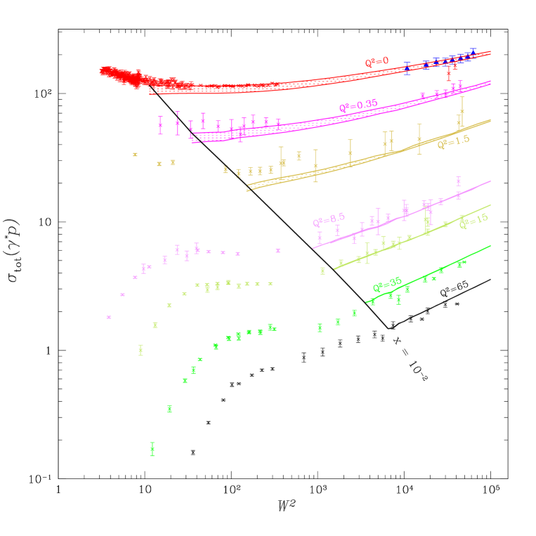
Figure 5: $\sigma(\gamma^{*}p)$ as a function of $W^{2}$ together with the experimental data. The full triangles correspond to data points which have been extracted in [19] from experimental data.

In Fig. 5 we show the results of our calculation for $\sigma(\gamma^{*}p)$ as a function of $W^{2}$ for fixed values of $Q^{2}$, together with the published experimental results. The calculated results are shown as a band which corresponds to the two limits on $M_{0,T}$. It is clear from the figure that the width of the band decreases with increasing $Q^{2}$. As for the longitudinal separation parameter, the results are not sensitive to the choice of $M_{0,L}$, and in all our calculations we simply used $M_{0,L}=2m_{\pi}$. The thick line marks the region of small $x$: to the left of it, $x$ is not small enough to justify using our model. One can see that for $x<10^{-2}$, our results reproduce the experimental results both in value and in energy dependence.

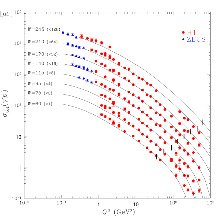
Figure 6: $\sigma(\gamma^{*}p)$ as a function of $Q^{2}$ together with the experimental data.

In Fig. 6 we show our calculations for $\sigma(\gamma^{*}p)$ for fixed values of $W^{2}$, as a function of $Q^{2}$, scaled by factors of $1-128$. The small vertical thick lines delineate the boundary $x=10^{-2}$, to the right of the marks our results are not reliable.

Figure 7: The ratio of $\displaystyle{\frac{\sigma_{\mbox{\scriptsize L}}}{\sigma_{\mbox{\scriptsize T}}}}$ as a function of $x$.

The longitudinal component of $\sigma(\gamma^{*}p)$, according to our calculation, reaches a maximum value of 25% of the total cross section at $x\approx 10^{-2}$. For small $x$, this result is closer to the published data [20] than the results of Ref. [10], where they obtained $\sigma_{\mbox{\scriptsize L}}$ for $x\approx 10^{-2}$ to be 15% of the total cross section. The ratio of the longitudinal cross section to the transverse cross section, as a function of $x$, is shown in Fig. 7 together with the (small $x$) data of Ref. [20].

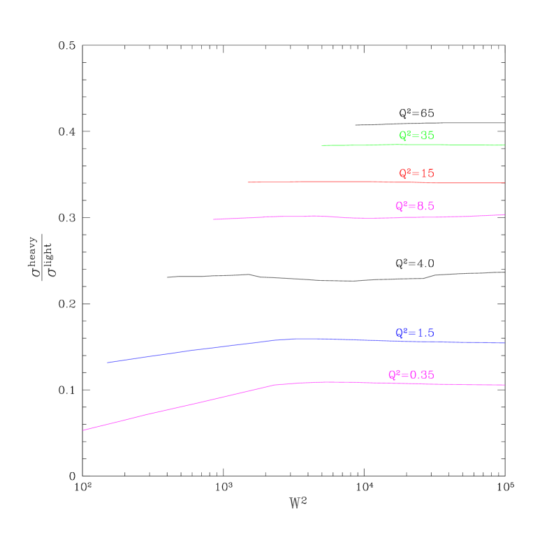
Figure 8: The ratio of $\frac{\sigma^{\mbox{\scriptsize heavy}}}{\sigma^{\mbox{\scriptsize light}}}$ at fixed $Q^{2}$.

Fig. 8 illustrates the importance of the heavy quarks contributions $\sigma^{\mbox{\scriptsize hard}}_{\mbox{\scriptsize T},\bar{Q}Q}$ and $\sigma^{\mbox{\scriptsize hard}}_{\mbox{\scriptsize L},\bar{Q}Q}$ [see Eqs. (24) and (33)]. The contribution has a mild $W^{2}$-dependence but it is $Q^{2}$-dependent, and for large $Q^{2}$, the ratio $\sigma^{\mbox{\scriptsize heavy}}/\sigma^{\mbox{\scriptsize light}}$ gets as high as $0.3-0.4$ . Another ratio which we present is the ratio, of the hard to the soft contributions. Since $M_{0,L}$ is smaller than the lightest resonance mass, the AQM contribution to the longitudinal component is supressed, and therefore what we call “soft” contribution is actually the transverse AQM calculation.

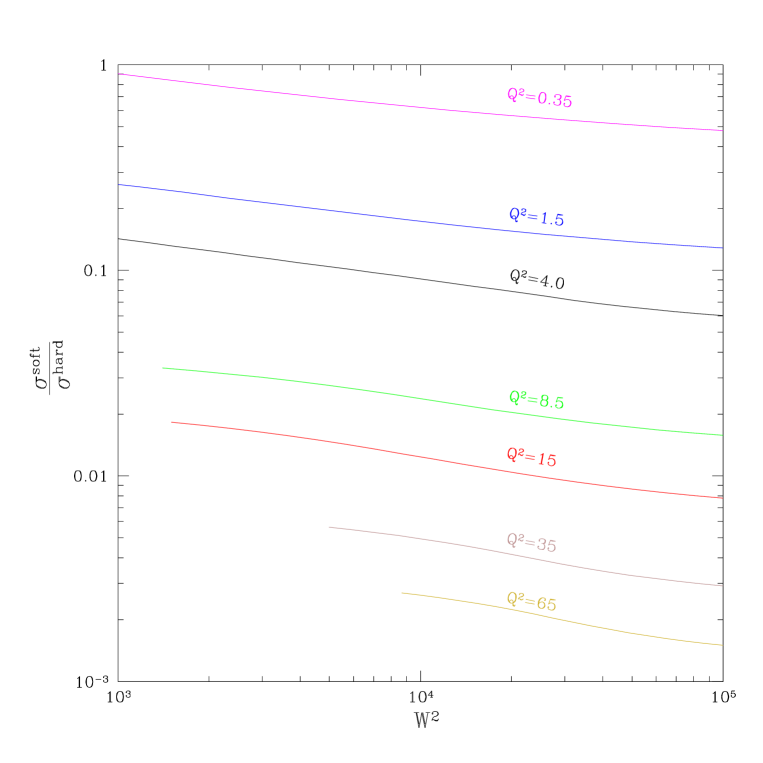
Figure 9: The ratio of $\frac{\sigma^{\mbox{\scriptsize soft}}}{\sigma^{\mbox{\scriptsize hard}}}$ at fixed $Q^{2}$.

In Fig. 9 we present the ratio $\sigma^{\mbox{\scriptsize soft}}/\sigma^{\mbox{\scriptsize hard}}$ at fixed values of $Q^{2}$, where a clear power law behaviour as a function of $W^{2}$ can be seen. In soft processes, the hard contribution is minor, but is still present even for relatively small values of $Q^{2}$. The soft signature in hard processes is also present, but is smaller. For high virtualities it decreases from a few precent at low energy, to less than 1% at high energies.

4 Conclusions

In this paper, we have shown that an approach based on Gribov’s proposal, provides a successful description of the experimental data on photon-proton interaction, over a wide range of photon virtualities $0\leq Q^{2}\leq 100\,{\,\mbox{GeV}^{2}}$, and energies $3\leq\sqrt{s}\,(=W)\leq 300$ GeV. The key assumption on which our aproach is based, is that the non-perturbative and the perturbative QCD conributions in the Gribov formula can be separated by the parameter $M_{0}$. Oue successful reproduction of the experimental data (see Figs. 5 and 6) shows that this assumption appears to be valid. It further lends credence to using the additive quark model (AQM) to describe the non-perturbative contribution. The successful use of the AQM leads to an improved result presented in this paper, compared to our previous result[6], where we found it necessary to introduce an damping factor for the AQM.

The second important by-product of our calculation is the simple method we have used to separate between non-perturbative (“soft”) and perturbative (“hard”) contributions. We have used three separation parameters: $M_{0,T}$, $M_{0,L}$ and $\mu$. The values of these parameters, $M^{2}_{0,T}=0.7-0.9\,{\,\mbox{GeV}^{2}}$, $M^{2}_{0,L}\leq 0.4\,{\,\mbox{GeV}^{2}}$ and $\mu^{2}\approx 1\,{\,\mbox{GeV}^{2}}$, were determined by fitting to the experimental data. We believe that these values may be useful in the future, for more theoretical description of the matching between “soft” and “hard” processes in QCD.

The third result which we find interesting, is that the GRV parameterizations of the structure functions cannnot successfully describe the experimental energy dependence of the total cross section at small values of $Q^{2}$ (see Fig. 4), while the MRST parameterizations can. This result shows the interdependence of deep inelastic scattering data, and the theoretical description of the mathching of the “soft” and “hard” contributions.

In addition we obtain:

1. A description of the ratio $\sigma_{\mbox{\scriptsize L}}/\sigma_{\mbox{\scriptsize T}}$ (see Fig. 7) which is in good agreement with the experimental data and other approaches. The fact that $\sigma_{L}$ appears to have only a “hard” contribution should be stressed, as this could be a possible window for particular features of non-pertutbative QCD;

2. A considerable contribution of the “soft” processes at rather large values of photon virtualities $Q^{2}$. For example at $Q^{2}=15\,{\,\mbox{GeV}^{2}}$, $\sigma^{\mbox{\scriptsize soft}}/\sigma^{\mbox{\scriptsize hard}}\,\approx\,\,4\%$ at $W=10\,GeV$ (see Fig. 9). We also find, at low $Q^{2}$, a contamination of the “soft” processes by the “hard” ones. For high energy real photoproduction this contamination amounts to about 5% . We believe that this fact should be taken into account when interpreting experimental data, especially as far as their energy dependance is concerned;

3. The prediction of the cross section for the heavy quark production (see Fig. 8) which is almost $W$ independent, while showing a steep $Q^{2}$ decrease.

We propose a simple and successful phenomenological model for the photon-proton interaction, which provides a method for matching the “soft” and “hard” interactions at high energy, and which can be a guide for future theoretical approaches. It is worthwhile mentioning, that even in the present form our model can be useful for determining the initial parton distributions at leading twist, for the DGLAP evolution equations.

Acknowledgments:

We thank A. Martin and A. Stasto for useful discussions of the results of this paper, and for providing us the kumac file for Fig.6. This research was supporteed in part by the Israel Science Foundation, founded by the Israel Academy of Science and Humanities.

References

-
[1]
H1 Collaboration: C. Adloff et al., Nucl. Phys. B497 (1997) 3;
H1 Collaboration: S. Aid et al., Nucl. Phys. B470 (1996) 3. - [2] ZEUS Collaboration: J. Breitweg et al., Phys. Lett. B407 (1997) 432.
- [3] V.N. Gribov, Sov. Phys. JETP 30 (1970) 709
-
[4]
J.J. Sakurai and D. Schildknecht, Phys. Lett. B40 (1972) 121
B. Gorczyca and D. Schildknecht, Phys. Lett. B47 (1973) 71. - [5] Particle Data Group, Eur. Phys. J. C3 (1998) 1.
- [6] E. Gotsman, E.M. Levin and U. Maor, Eur. Phys. J.C5 (1998) 303
- [7] B. Badelek and J. Kwiecinski, Z. Phys. C43 (1989) 251, Phys. Lett. B295 (1992) 263, Phys. Rev. D50 (1994) R4.
-
[8]
E.M. Levin and L.L. Frankfurt, JETP Letters 3 (1965) 652;
H.J. Lipkin and F. Scheck, Phys. Rev. Lett. 16 (1966) 71;
J.J.J. Kokkedee, The Quark Model , NY, W.A. Benjamin, 1969. - [9] A. Donnachie and P.V. Landshoff, Nucl. Phys. B244 (1984) 322, Nucl. Phys. B267 (1986) 690, Phys. Lett. B296 (1992) 227, Z. Phys. C61 (1994) 139.
- [10] A.D. Martin, M.G. Ryskin and A.M. Stasto, DTP/98/20; hep-ph/9806212.
- [11] K. Colec - Biermat and M. Wüsthoff, Phys. Rev. D59 (1999) 014017.
- [12] H. Abramowicz, E. Levin, A. Levy and U. Maor, Phys. Lett. B269 (1991) 465.
- [13] H. Abramowicz and A. Levy, DESY 97-251, hep-ph/9712415.
- [14] E. M. Levin, A. D. Martin, M. G. Ryskin and T. Teubner, Z. Phys. C74 (1997) 671.
- [15] D. Schildknecht, H. Spiesberger, BI-TP 97/25, hep-ph/9707447.
- [16] M. Gluck, E. Reya and A. Vogt, Z. Phys. C67 (1995) 433.
- [17] M. Gluck, E. Reya and A. Vogt, hep-ph/9806404.
- [18] A.D. Martin, R.G. Roberts, W.J. Stirling and R.S. Thorne: “Parton distributions: a new global analysis”, DTP/98/10; hep-ph/9803445.
- [19] ZEUS Collaboration: J. Breitweg et al., DESY 98-121, hep-ex/9809005.
- [20] NMC Collaboration, Nucl. Phys. B483 (1997) 3.