Simulating hot Abelian gauge dynamics

Abstract

The time evolution of soft modes in a quantum gauge field theory is to first approximation classical, but the equations of motion are non-local. We show how they can be written in a local and Hamiltonian way in an Abelian theory, and that this formulation is particularly suitable for numerical simulations. This makes it possible to simulate numerically non-equilibrium processes such as the phase transition in the Abelian Higgs model and and to study, for instance, bubble nucleation and defect formation. This would also help to understand the phase transitions in more complicated gauge theories. Moreover, we show that the existing analytical results for the time-evolution in a pure-gauge theory correspond to a special class of initial conditions and that different initial conditions can lead to qualitatively different behavior. We compare the results of the simulations to analytical calculations and find an excellent agreement.

I Introduction

The recent finding that the electroweak phase transition might be only a smooth crossover [1] has changed the picture of cosmological phase transitions in a fundamental way and shown that theories with gauge fields can behave very differently from those with only global symmetries. However, the statement about the smoothness of the transition refers only to the equilibrium properties, and from the point of view of cosmology, it is very important to understand also the time evolution of the transition, in particular, whether the fields fall out of equilibrium and what its consequences would be. For this, a calculation scheme is needed for dynamical quantities that treats the gauge fields correctly and gives the same results in the special case of thermal equilibrium as the the dimensional reduction method [2, 3] that was used to show the smoothness of the electroweak transition. In this paper, we propose such a scheme.

Instead of the electroweak theory, we will concentrate here on scalar electrodynamics, i.e. the Abelian Higgs model. Not only does the simpler gauge group allow more efficient simulations, but the theory also contains topological defects, namely Nielsen-Olesen vortices [4], and therefore it can be used to simulate defect formation in a phase transition [5] and to test the validity of the present predictions for the produced defect density [6] in gauge theories.

In Ref. [7], the dynamics of the transition and, in particular, formation of vortices was simulated classically on a lattice with field equations derived from the original Lagrangian. A similar approach had been suggested earlier [8] in the context of electroweak baryogenesis. This was based on the observation that the quantum distribution of the long-wavelength modes is essentially classical. Since the time evolution of a classical field theory is given by the equations of motion, this approach allows non-perturbative numerical simulations. For baryogenesis, the interesting quantity is the hot sphaleron rate (see Ref. [9] and references therein), which is an equilibrium quantity, but similar methods can also be used to describe small deviations from equilibrium, such as phase transitions. After all, the phase of the system is only a property of the long-wavelength modes, and the distribution of the high-momentum modes is to a large extent independent of it. Therefore also the transition between the phases is described by the classical long-wavelength modes.

This straightforward approach has the serious problem that the results depend on the ultraviolet cutoff[10, 11]. Because of the Rayleigh-Jeans ultraviolet divergences, a classical continuum field theory cannot actually even be in thermal equilibrium – this was one of the reasons why quantum mechanics was invented in the first place! The divergences depend on the temperature and are absent at zero temperature, so they cannot be cancelled by introducing counterterms as in quantum theories. Therefore it is not sufficient to use the classical theory with the Lagrangian of the original quantum theory, but one has to construct an effective Lagrangian for the low-momentum (soft) modes by integrating out the high-momentum (hard) modes. The effective Lagrangian then contains precisely the necessary (temperature-dependent) counterterms to remove the divergences.

In calculating static properties, i.e. expectation values of products of operators measured at the same time, this procedure is known as dimensional reduction[2], and leads to a three-dimensional effective theory, in which the temporal component of the gauge field has a Debye mass term $m_{D}\sim gT$. To calculate non-static quantities, the full four-dimensional effective Lagrangian needs to be constructed by calculating the so-called hard thermal loops, and in gauge theories it turns out to be non-local [12, 13]. This makes computer simulations practically impossible, since one would have to keep in the memory all the configurations encountered during the time evolution.

Fortunately, the equations of motion can be written in a local form by introducing auxiliary fields[14, 15]. The Abelian version of the resulting system of differential equations is known in plasma physics as the Vlasov equation and describes collisionless electron plasma. Numerical solution of the equations of motion is still difficult, since the field $W$ depends not only on the coordinate but also on the momenta of the hard particles it describes, and therefore the theory becomes essentially five-dimensional. The traditional method is to approximate it by a large number of point particles. This approach has been used to determine the hot sphaleron rate in the electroweak theory in Ref. [16].

In this paper, we show how the theory can be formulated in such a way that simulations in terms of fields rather than particles becomes feasible. One of the problems we have to face is the multiplication of the number of degrees of freedom when the hard modes are included. We show that the number of extra degrees of freedom per lattice site must be chosen carefully if the simulation of a particular soft mode is to be trusted: if one wants to reproduce Landau damping in a mode of momentum $k$, naive methods require of order $(kt)^{2}$ degrees of freedom per lattice site for the hard modes. However, we are able to rewrite the effective hard thermal loop improved classical equations of motion in such a way that we only need of order $kt$ extra degrees of freedom per lattice site. Our numerical methods reproduce known analytic results in pure Abelian gauge theory extremely well, which gives us confidence that we will be able to tackle the Abelian Higgs model accurately.

The structure of the paper is the following. In Sec. II we review the hard thermal loop Lagrangian and derive the Hamiltonian formulation for the hard modes. In Sec. III we explain how to approximate the system with a finite number of degrees of freedom in numerical simulations. In Sec. IV we derive some analytical results, which we compare to our numerical results in Sec. V. Extending our technique to include the soft Higgs field is discussed in Sec. VI, and Sec. VII contains the conclusions. The paper also has one appendix, in which the continuum and lattice equations of motion for the Legendre modes are given explicitly.

II Kinetic formulation

Let us consider scalar electrodynamics at a temperature $T$. The Lagrangian of the theory is

$${\cal L}=-\frac{1}{4}F_{\mu\nu}F^{\mu\nu}+|D_{\mu}\phi|^{2}-m^{2}|\phi|^{2}-\lambda|\phi|^{4},$$ (1)

where $D_{\mu}=\partial_{\mu}+ieA_{\mu}$. We assume that $e\ll 1$ and $\lambda\sim e^{2}$ and that $m\ll T$ so that high-temperature approximation can be used.

The phase structure of the theory was determined in Refs. [17, 18]. When the Higgs self-coupling is small, there is a first-order phase transition, but if the self-coupling is large enough, the transition becomes continuous. Unlike in the electroweak theory, it does not become a smooth crossover. In Ref. [19], it was pointed out that this can be interpreted as a consequence of the existence of Nielsen-Olesen vortices.

To one-loop order, the only non-vanishing contributions to the effective Lagrangian arise from the two-point diagrams. The correct procedure would be to calculate the diagrams in the original quantum theory and to write down a classical Lagrangian that gives the same result when the diagrams are calculated on a lattice [10]. However, this is not possible in practice, since the form of the necessary effective lattice Lagrangian is not known and is presumably very complicated because the lattice has much less symmetry than the continuum. In sphaleron rate calculations, the effective Lagrangian was taken from the continuum theory and the parameters were fixed by matching only the static quantities [16]. For the simulations presented in this paper, this problem does not arise, as will be discussed later.

In the high-temperature approximation, the one-loop scalar self-energy is simply

$$\Sigma=-\left(\frac{e^{2}}{4}+\frac{\lambda}{3}\right)T^{2}.$$ (2)

The photon self-energy [20] is more complicated and if the external momentum is $K=(\omega,\vec{k})$, it can be written in the form

$$\Pi^{\mu\nu}=\Pi_{T}P_{T}^{\mu\nu}+\Pi_{L}P_{L}^{\mu\nu},$$ (3)

where $P_{T}^{\mu\nu}$ and $P_{L}^{\mu\nu}$ are the spatially transverse and longitudinal projection operators

$$P_{T}^{ij}=\frac{k^{i}k^{j}}{k^{2}}-\delta^{ij},\quad P_{T}^{\mu 0}=0,\quad P_{L}^{\mu\nu}=g^{\mu\nu}-\frac{K^{\mu}K^{\nu}}{K^{2}}-P_{T}^{\mu\nu},$$ (4)

and

$$\Pi_{L}=m_{D}^{2}\left(1-\frac{\omega^{2}}{k^{2}}\right)\left(1-\frac{\omega}{2k}\ln\frac{\omega+k}{\omega-k}\right),\quad\Pi_{T}=\frac{1}{2}\left(m_{D}^{2}-\Pi_{L}\right).$$ (5)

The Debye mass has the value $m_{D}^{2}=\frac{1}{3}e^{2}T^{2}+\delta m_{D}^{2}$, where $\delta m_{D}^{2}$ is a cutoff-dependent counterterm.

The self-energies can be resummed to a simple effective Lagrangian for the soft modes

$${\cal L}_{\text{HTL}} = -\frac{1}{4}F_{\mu\nu}F^{\mu\nu}-\frac{1}{4}m_{D}^{2}\int\frac{d\Omega}{4\pi}F^{\mu\alpha}\frac{v_{\alpha}v^{\beta}}{(v\cdot\partial)^{2}}F_{\mu\beta}$$ (7)

$$+|D_{\mu}\phi|^{2}-m_{T}^{2}|\phi|^{2}-\lambda|\phi|^{4},$$

where $m_{T}^{2}=m^{2}+(e^{2}/4+\lambda/3)T^{2}+\delta m_{T}^{2}$, and the integration is taken over the unit sphere of velocities $v=(1,\vec{v})$, $\vec{v}^{2}=1$. Note that the form of $m_{T}^{2}$ justifies using the high-temperature approximation even slightly below the transition. At tree level, the transition takes place when $m_{T}^{2}=0$, which shows that $m^{2}\sim-e^{2}T_{c}^{2}$. The minimum of the potential is therefore at $v\sim T_{c}$, and the mass given by the Higgs mechanism is $m_{H}^{2}\sim e^{2}T_{c}^{2}\ll T^{2}$.

The equations of motion derived from the Lagrangian (7) are

$$\partial_{\mu}F^{\mu\nu} = m_{D}^{2}\int\frac{d\Omega}{4\pi}\frac{v^{\nu}v^{i}}{v\cdot\partial}E^{i}-2e{\rm Im}\phi^{*}D^{\nu}\phi,$$ (9)

$$D_{\mu}D^{\mu}\phi = -m_{T}^{2}\phi-2\lambda(\phi^{*}\phi)\phi.$$ (10)

The derivative in the denominator in Eq. (9) means that in order to simulate it numerically, one needs to keep the whole time evolution of the system in the memory at the same time, which is impossible. The form of the equation of motion (10) of the scalar field is much simpler, and actually the only effect of the hard modes is the modified mass term. The scalar field can therefore be simulated with standard methods and we will neglect it from now on, concentrating only on the gauge field. We will refer to this theory as the pure gauge theory although it contains the contribution from the hard scalar modes.

The non-locality problem of Eq. (9) can be solved by introducing new fields[14, 15]. We follow Ref.[15] and add the field $W(x,\vec{v})$, which satisfies the equation of motion

$$(v\cdot\partial)W(x,\vec{v})=\vec{v}\cdot\vec{E}(x),$$ (11)

and replacing Eq. (9) with

$$\partial_{\mu}F^{\mu\nu}=j_{W}^{\nu}(x)+j^{\nu}(x),$$ (12)

where

$$j_{W}^{\nu}(x)=m_{D}^{2}\int\frac{d\Omega}{4\pi}v^{\nu}W(x,\vec{v}),$$ (13)

and $j^{\nu}(x)$ denotes the current due to the scalar field and any external currents.

The system of equations (11), (12) is a special case of what is known as the Vlasov equation in plasma physics, where it describes collisionless electron plasma. The field $W(x,\vec{v})$ gives the deviation of the density of hard particles of velocity $\vec{v}$ from their equilibrium distribution.

In addition to the equations of motion, we also have to specify the initial conditions, and since we would like to have the system initially in a thermal equilibrium, they should be given by the equilibrium distribution, i.e. we should have a large number of initial configurations with a Boltzmann distribution $\propto\exp(-\beta H)$, where $H$ is the Hamiltonian. However, the equation of motion (11) for the $W$ field is not of canonical form, which makes it difficult to find the correct Hamiltonian. The suggestion of[21] was to use the conserved quantity

$$H=\frac{1}{2}\int d^{3}x\left\{\vec{E}^{2}+\vec{B}^{2}+m_{D}^{2}\int\frac{d\Omega}{4\pi}W(x,\vec{v})^{2}\right\}.$$ (14)

In the simulations, one has to approximate the system with a finite number of degrees of freedom. Normally, this is done by discretizing the space to a finite lattice, but in our case, the field $W$ also depends on a two-dimensional continuous parameter $\vec{v}$. There are various ways to handle it in simulations. In Refs. [16, 22], $W$ was approximated with a large number of particles. The other straightforward options are approximating the velocity integral with a discrete set of velocities on the unit sphere, or expanding $W$ in terms of spherical harmonics. However, as we will show next, at least in the Abelian case it pays to simplify the problem a bit first.

Let us define in Fourier space

$$\vec{f}(\omega,\vec{k},z) = im_{D}\sqrt{\frac{2z^{2}}{1-z^{2}}}\int\frac{d\Omega}{4\pi}\frac{\vec{v}\times\vec{k}}{(\vec{v}\cdot\vec{k})^{2}}W(\omega,\vec{k},\vec{v})\left(\delta(\vec{v}\cdot\hat{k}-z)+\delta(\vec{v}\cdot\hat{k}+z)\right)$$ (16)

$$-\frac{im_{D}}{k^{2}}\sqrt{\frac{1-z^{2}}{2z^{2}}}\vec{k}\times\vec{A},$$

$$\theta(\omega,\vec{k},z) = im_{D}\int\frac{d\Omega}{4\pi}\frac{1}{\vec{v}\cdot\vec{k}}W(\omega,\vec{k},\vec{v})\left(\delta(\vec{v}\cdot\hat{k}-z)+\delta(\vec{v}\cdot\hat{k}+z)\right)+\frac{im_{D}}{k^{2}}\vec{k}\cdot\vec{A}.$$ (17)

Then the equations of motion in the temporal gauge $A_{0}=0$ are

$$\partial_{0}^{2}{\vec{f}}(z) = z^{2}\vec{\nabla}^{2}\vec{f}+m_{D}z\sqrt{\frac{1-z^{2}}{2}}\vec{\nabla}\times\vec{A},$$ (19)

$$\partial_{0}^{2}{\theta}(z) = z^{2}\vec{\nabla}\cdot\left(\vec{\nabla}\theta-m_{D}\vec{A}\right),$$ (20)

$$\partial_{0}^{2}{\vec{A}} = -\vec{\nabla}\times\vec{\nabla}\times\vec{A}+m_{D}\int_{0}^{1}dzz^{2}\left(\vec{\nabla}\theta-m_{D}\vec{A}+\sqrt{\frac{1-z^{2}}{2z^{2}}}\vec{\nabla}\times\vec{f}\right)+\vec{j}.$$ (21)

One advantage of this formulation is that these equations of motion are canonical and the corresponding Hamiltonian is

$$H = \frac{1}{2}\int d^{3}x\int_{0}^{1}dz\Biggl{[}\vec{E}^{2}+(\vec{\nabla}\times\vec{A})^{2}+\vec{F}^{2}+{\Pi}^{2}+z^{2}(\vec{\nabla}\times\vec{f})^{2}+z^{2}(\vec{\nabla}\theta-m_{D}\vec{A})^{2}$$ (23)

$$-m_{D}z\sqrt{\frac{1-z^{2}}{2}}\vec{f}\cdot\vec{\nabla}\times\vec{A}\Biggr{]},$$

where $\vec{F}=\partial_{0}{\vec{f}}$ and $\Pi=\partial_{0}\theta$ are the canonical momenta of $\vec{f}$ and $\theta$, respectively. We also need two extra conditions, namely the transverseness of $\vec{f}$ and Gauss’s law

$$\vec{\nabla}\cdot\vec{f} = \vec{\nabla}\cdot\vec{F}=0,$$ (24)

$$\vec{\nabla}\cdot\vec{E} = -m_{D}\int_{0}^{1}dz\Pi(z).$$ (25)

By reformulating the degrees of freedom, we have gained two important advantages. First, $\vec{f}$ depends only on one internal coordinate whereas $W$ depends on two, and second, since we know the Hamiltonian (23), we know the correct distribution of the initial configurations.

III Simulations

We still have to approximate the $z$-dependence of the hard modes with a finite number of degrees of freedom, and we will use Legendre polynomials for that. We define

$$\vec{f}^{(n)} = \int_{0}^{1}dzz\sqrt{\frac{1-z^{2}}{2}}P_{2n}(z)\vec{f}(z),$$ (26)

$$\theta^{(n)} = \int_{0}^{1}dzz^{2}P_{2n}(z)\theta(z),$$ (27)

where $P_{n}(z)$ is the $n$th Legendre polynomial. The equations of motion for different Legendre modes are given in Eq. (A5) in the appendix. It is also shown in the appendix that the approximation can be trusted if the simulation time is less than

$$t_{0}\approx 2N_{\text{max}}/k.$$ (28)

On the lattice, the field $\theta$ is defined on lattice sites, while $\vec{f}$ and the gauge field $\vec{A}$ are defined on links between the sites in such a way that the invariance under time-independent gauge transformations is preserved. Note that the field $\theta^{(0)}$ is not gauge invariant by itself, but the combination $\vec{\nabla}\theta^{(0)}-\frac{1}{3}m_{D}\vec{A}$ is. The canonical momenta are defined at half-way between the time steps so that the value of, say, $\vec{f}$ at time $t+\delta t$ is determined from the fields at time $t$ and the momenta at time $t+\delta t/2$. In this way, the time reversal invariance of the continuum theory is preserved. The lattice equations of motion are given in Eq. (A18) in the appendix.

The aim of the simulations described here was mainly to test the simulation code by comparing it with known analytical results. Therefore we neither averaged over thermal initial conditions nor included the scalar field. The equations of motion for the pure gauge theory are linear and can therefore in principle be solved analytically. It also means that the modes with different momenta do not interact with each other, and to simulate a mode with momentum along, say, the $z$ axis, we can use a lattice with $1\times 1\times N_{z}$ sites. This makes the simulations very simple. Moreover, the pure gauge theory is ultraviolet finite, so no mass counterterms are needed. In particular, $\delta m_{D}^{2}$ and $\delta m_{T}^{2}$ introduced in Sec. II vanish.

IV Analytical Results

Before specializing to particular solutions, we first discuss the finite temperature propagator for the pure Abelian theory. Due to linearity, it is sufficient to consider a single Fourier mode at a time. Let the momentum be $\vec{k}$, and, for simplicity, let us consider just the transverse part of the propagator $G(t,\vec{x})$. Its Fourier transform has a non-analytic form

$$\frac{1}{G(\omega,\vec{k})}=-\omega^{2}+k^{2}+\frac{m_{D}^{2}}{4}\left[2\frac{\omega^{2}}{k^{2}}+\frac{\omega}{k}\frac{k^{2}-\omega^{2}}{k^{2}}\ln\frac{\omega+k}{\omega-k}\right].$$ (29)

The analytic structure of the propagator is shown in Fig. 1. The propagator has two oscillatory poles on the real axis at $\omega^{2}_{p}\approx k^{2}+\frac{1}{3}m_{D}^{2}$, but also a branch cut from $\omega=-k$ to $\omega=k$. The original equation of motion (9) implies that the branch cut must be taken along the real axis. There are no other singularities on this physical Riemann sheet, but if one continues the propagator analytically from the upper half-plane through the branch cut, one finds a pole at

$$\omega=-i\gamma_{L}\approx-i\frac{4k^{3}}{\pi m_{D}^{2}}.$$ (30)

Likewise, continuing analytically from the lower half-plane through the cut reveals a pole at $\omega=i\gamma_{L}$.

The solution to the inhomogeneous equation with an external source $\vec{j}(\omega)$ is, assuming that the current is transverse and that the fields vanish at $t=-\infty$,

$$\vec{A}(t,\vec{k})=\int_{-\infty+i\epsilon}^{\infty+i\epsilon}\frac{d\omega}{2\pi}e^{-i\omega t}G(\omega)\vec{j}(\omega).$$ (31)

If $t>0$, the integral can be transformed into a contour integral by closing it on the lower half-plane. This integral has three pieces: two contributions from the poles and one from the integral around the branch cut. The result of the integration around the cut is sensitive to the functional form of $\vec{j}(\omega)$, a reflection of the non-locality of Eq. (9): the behavior of the system depends on its whole history.

For example, Boyanovsky et al. [23] discussed a situation in which an inhomogeneous initial configuration is set up for the soft fields $\vec{A}$ and $\vec{E}$, and calculated its relaxation to the equilibrium at asymptotically long times. Still keeping the assumption of transverseness, the solution was given as a function of $\vec{A}$ and $\vec{E}$ at time $t=0$,

$$\vec{A}(t,\vec{k}) \approx \vec{A}(0,\vec{k})\left[Z[T]\cos\omega_{p}t-\frac{4}{m_{D}^{2}}\frac{\cos kt}{t^{2}}\right]-\vec{E}(0,\vec{k})\left[Z[T]\frac{\sin\omega_{p}t}{\omega_{p}}-\frac{4}{m_{D}^{2}}\frac{\sin kt}{kt^{2}}\right],$$ (32)

where

$$Z[T]=-\left(\frac{\partial G^{-1}}{\partial\omega^{2}}\right)^{-1}_{\omega=\omega_{p}}.$$ (33)

Eq. (32) can be seen to correspond to $\vec{j}(\omega)=-i\omega\vec{A}(0)-\vec{E}(0).$ As they emphasize, the dominant contribution does not come from the smallest frequencies but those near the end points of the branch cut.

With a different choice of $\vec{j}$, qualitatively different solutions can be found. Suppose that $\vec{j}(t)$ is increased very slowly from zero to a finite value and then suddenly switched off, i.e. $\vec{j}(t)=\vec{j}_{0}e^{\gamma_{0}t}\Theta(-t)$, where $\gamma_{0}$ is eventually taken to zero and $\Theta(t)$ is the step function. The Fourier transform $\vec{j}(\omega)=\vec{j}_{0}/(\gamma_{0}+i\omega)$ is peaked around the origin, and therefore the integral around the branch cut is dominated by the integrand near $\omega=0$. Hence, expanding the propagator around $\omega=i\epsilon$ and $\omega=-i\epsilon$ on the upper and lower half-planes, respectively, we may write

$$\left.\vec{A}(t,\vec{k})\right|_{\rm cut}\approx\vec{j}_{0}\int_{-k}^{k}\frac{d\omega}{2\pi}\left(e^{-i\omega t}\frac{1}{\gamma_{0}+i\omega}\frac{1}{\gamma_{L}-i\omega}+e^{i\omega t}\frac{1}{\gamma_{0}-i\omega}\frac{1}{\gamma_{L}-i\omega}\right)\frac{\gamma_{L}}{k^{2}}.$$ (34)

The limits of the integral may be taken to infinity, and the contour closed in either the upper or the lower half-plane depending on the sign of the exponent. The second term has no poles in the upper half-plane and hence vanishes, while the first term gets a contribution from the pole at $\omega=-i\gamma_{L}$. Thus we find an exponentially damping solution

$$\left.\vec{A}(t,\vec{k})\right|_{\rm cut}\approx-\frac{\vec{j}_{0}}{k^{2}}e^{-\gamma_{L}t}.$$ (35)

This exponential decay is known as Landau damping, and it is important to notice that it did not really come from integrating around a pole of the propagator (29). If it had, then the equations of motion would either have to break time reversal invariance, which they do not do, or there would have to be a corresponding exponentially growing solution, thus making the system unstable.

For completeness, we also calculate the contribution coming from the poles at $\omega=\pm\omega_{p}$. The full result is then

$$\vec{A}(t,\vec{k})\approx-\vec{j}_{0}\left(Z[T]\frac{\cos\omega_{p}t}{\omega_{p}^{2}}+\frac{1}{k^{2}}e^{-\gamma_{L}t}\right).$$ (36)

V Numerical results

In order to numerically reproduce the results (32), (36), we have to specify the correct initial conditions in terms of $\vec{f}$ and $\theta$. The result (32) is given simply by $\vec{f}(0)=\theta(0)=0$. For the soft modes, we chose $\vec{A}(0)=0$, $\vec{E}(0)=10\hat{y}\sin\vec{k}\cdot\vec{x}$. To see the power-law damping most clearly, $m_{D}$ must be relatively small, and we chose $m_{D}=2\pi$, $\vec{k}=2\pi\hat{x}$ in our units. The lattice size was $20\times 1\times 1$, lattice spacing $a=0.05$ and the time step $\delta t=0.01$. We used $N_{\rm max}=200$ so that according to Eq. (28) the results should be reliable when $t\lesssim 60$. Eq. (32) becomes

$$\vec{A}(t,\vec{k})\approx\left(-1.236\sin 7.451x+0.1613\frac{\sin 2\pi t}{t^{2}}\right)\hat{y}.$$ (37)

We added to the numerical result a constant-amplitude part $\alpha\sin\beta t$ and determined the parameters $\alpha$ and $\beta$ from the condition that the remaining part agrees with the decaying part of Eq. (37). The result with $\alpha=1.24008$ and $\beta=7.43024$ is shown in Fig. 2. The discrepancy between the numerical and analytical results is less than one percent.

The initial conditions that correspond to Eq. (36) are those in which the first and second time derivatives of the fields vanish. If we choose $\vec{j}_{0}$ such that $\vec{A}(0,\vec{x})=\hat{y}\sin\vec{k}\cdot\vec{x}$, then Eqs. (17) and (27) imply that

$$\vec{f}^{(0)}(0,\vec{x}) = \frac{m_{D}}{3k}\hat{z}\cos\vec{k}\cdot\vec{x},$$ (38)

$$\vec{f}^{(1)}(0,\vec{x}) = -\frac{m_{D}}{15k}\hat{z}\cos\vec{k}\cdot\vec{x},$$ (39)

$$\vec{f}^{(n>1)}(0,\vec{x}) = 0,\quad\theta^{(n)}(0,\vec{x})=0.$$ (40)

The exponential damping is seen most clearly if $m_{D}\gg k$, and we chose two different values $m_{D}=10\pi$ and $m_{D}=20\pi$ while we took again $\vec{k}=2\pi\hat{x}$. Again, the lattice size was $20\times 1\times 1$, the lattice spacing $a=0.05$, the time step $\delta t=0.01$, and $N_{\rm max}=200$. The results of the simulations are shown in Fig. 3. The predicted decay rates are $\gamma_{L}=0.32$ and $\gamma_{L}=0.08$ and the amplitudes of the oscillation $A_{\rm osc}\approx 0.103$ and $A_{\rm osc}\approx 0.029$. As can be seen from Fig. 3, these agree very well with the numerical results.

We also carried out simulations with with different values of $N_{\rm max}$ to find out at what time the approximation breaks down and to test the estimate (28). We used $m_{D}=20\pi$ and the values for the other parameters were as before. Since all the Legendre modes with $n>1$ are initially zero, we expect the first errors to occur at time $t\approx 2t_{0}\approx 4N_{\rm max}/k$. The result is shown in Fig. 4 for various values of $N_{\rm max}$ and confirms our estimate. The number of extra scalar degrees of freedom needed for simulating with any particular value of $N_{\rm max}$ is $8N_{\rm max}$.

In order to compare the efficiency of the Legendre polynomial formulation with other approaches, we carried out the same simulations with a more straightforward method. We chose a large number of points on the unit sphere to represent different velocities and used them to simulate the pair of equations (11), (12). More precisely, the different velocities were

$$\vec{v}=\frac{(N_{v}+\frac{1}{2},n_{y},n_{z})}{\sqrt{(N_{v}+\frac{1}{2})^{2}+n_{y}^{2}+n_{z}^{2}}},\quad-N_{v}\leq n_{i}\leq N_{v},$$ (41)

and those obtained from that with reflections or rotations of $\pi/2$. The parameters were the same as in Fig. 4. The values of $N_{v}$ used ranged from 2 to 8, and the corresponding number of extra degrees of freedom is $6(2N_{v}+1)^{2}$. The results in Fig. 5 show clearly that the number of different velocities becomes quickly prohibitive when the simulation time is increased. If we assume that, as with the Legendre polynomials, the particularly smooth initial conditions result in a factor of two in the reliable simulation time, we can estimate that generally a simulation will be reliable if $t\lesssim\pi N_{v}/k$.

This estimate can also be reached analytically. Since the time evolution is a superposition of oscillations, the reliable simulation time is $t_{0}\approx\pi/\omega_{0}$, where $\omega_{0}$ is the smallest frequency, i.e. the pole of the propagator that is nearest to the origin. The transverse self-energy $\Pi_{T}(\omega)$ diverges if $\omega=\vec{k}\cdot\vec{v}$ for any velocity $\vec{v}$. The smallest pole of the propagator is at a frequency $\omega_{0}$, which is smaller than $\min\{\vec{k}\cdot\vec{v}\}$, but of the same order of magnitude. Generally $\min\{\vec{k}\cdot\vec{v}\}\approx k/N_{v}$, leading to the previous estimate.

Since expansion of $W$ in Eq. (11) in terms of spherical harmonics $Y^{m}_{n}$ is essentially equivalent to the expansion of $\vec{f}$ and $\theta$ in terms of Legendre polynomials, we can also estimate the effectiveness of that approach. In order to reach the same simulation time, the highest $n$ used should be $2N_{\rm max}$. The number of extra degrees of freedom would then be $(2N_{\rm max}+1)^{2}$, which again increases much faster than in the Legendre polynomial approach. Our estimates of the reliable simulation times in the different approaches have been summarized in table I. They show that the Legendre polynomial formulation is the most economical one.

VI Higgs model

The pure gauge theory that has been discussed so far is an ideal way to test the formalism, since it is linear and one can in principle solve it exactly. In the previous section, we have shown that the numerical results agree with the analytical calculations and we were even able to estimate the number $N_{\rm max}$ of Legendre modes needed to ensure that the simulation is reliable.

It is very easy to transform the system to a very non-trivial one simply by adding a Higgs field. While this makes it impossible to solve the equations of motion analytically, from the point of view of numerical simulations it means only adding one more field. Still, the resulting theory has a complicated structure with a phase transition and topological defects.

As was shown in Sec. II, the weak-coupling condition $e\ll 1$ and $\lambda\sim e^{2}$ implies that the hard thermal loop approximation is also valid near the transition in the broken phase. The reason is that the distribution of the hard modes is independent of the phase. Furthermore, when the phase transition takes place in a finite time, only the soft modes fall out of equilibrium, and therefore the classical description remains valid, even in such non-equilibrium processes.

The above suggests that the classical formalism discussed in this paper can be used to simulate non-equilibrium dynamics of the phase transition in hot scalar electrodynamics. In the cosmological setting the transition takes place when the universe cools as it expands, but in a simulation some other way to change the temperature is needed. A straightforward way of doing this is preparing an initial ensemble with a higher temperature for the soft modes than for the hard modes. A large number of initial configurations would then be taken from this ensemble and evolved in time. When the soft and hard modes interact, the temperature of the soft modes decreases and they undergo a phase transition.

While this kind of an instantaneous quench in the temperature is not very realistic, it would still be a first approximation to the true cosmological phase transition. These simulations would answer many interesting questions about the dynamics of the phase transition, for instance the density of topological defects created.

Certainly, the hard thermal loop approximation we have used is only valid at relatively short times. We have neglected the collisions of the hard particles and at long times $t\gtrsim 1/e^{4}T$ they would have an essential contribution to the time evolution [24]. If the coupling is weak, as we assume, this is not a serious problem. The other problem is to remove the effect of the ultraviolet lattice modes as discussed in Sec. II. The fact that the simulations of [7] showed no signs of a Rayleigh-Jeans catastrophe developing over the course of the simulation seems to indicate that the effect can safely be neglected.

Phase transitions and other non-equilibrium processes can be simulated also in non-Abelian theories using the Vlasov equation (11) to describe the hard modes. It would be important to know, whether a formulation analogous to Eq. (II) with only one internal coordinate is also possible in non-Abelian theories, since that would reduce the need of computational power drastically. Since the derivative in Eq. (11) is replaced with a covariant derivative, operating in the momentum space becomes more complicated and the same derivation cannot be used.

VII Conclusions

In this paper, we have studied hot Abelian gauge field theory in the hard thermal loop approximation. Starting from the local kinetic formulation (11), (12), we were able to reformulate the degrees of freedom in a more economical way. The equations of motion in the new formulation are canonical and we found the explicit form of the Hamiltonian (23).

The pure gauge theory discussed in this paper is linear and can therefore be solved analytically, at least in principle. We pointed out that because of non-locality it is not sufficient to specify the initial conditions for the soft modes only. In a sense, one will have to specify the whole history of the system in order to calculate its behavior in the future. Taking this effect into account modifies the existing results [23] and leads to exponential damping (36) with the Landau damping rate.

In order to simulate the system, we approximated the functions $\vec{f}$, $\theta$ with a finite number of Legendre polynomials. The simulations reproduced the analytical results, and the number of degrees of freedom needed to describe the hard modes was much smaller than in other possible approaches. This shows that the formulation presented in this paper is very well suited for numerical simulations.

While the pure gauge theory is trivial in the sense that it can be solved analytically, including the soft Higgs field makes analytical calculations essentially impossible. On the other hand, it is very simple to add it to numerical simulations. Leaving possible ultraviolet problems aside, that would give a way to study non-perturbatively the non-equilibrium dynamics of a phase transition in a gauge field theory.

A Equations of motion for Legendre modes

The equations of motion for the Legendre modes defined in Eq. (27) are

$$\partial_{0}^{2}{\vec{f}}^{(n)} = C^{+}_{n}\vec{\nabla}^{2}\vec{f}^{(n+1)}+C^{0}_{n}\vec{\nabla}^{2}\vec{f}^{(n)}+C^{-}_{n}\vec{\nabla}^{2}\vec{f}^{(n-1)}$$ (A2)

$$+m_{D}\vec{\nabla}\times\vec{A}\left(\frac{1}{15}\delta_{n,0}+\frac{1}{105}\delta_{n,1}-\frac{4}{315}\delta_{n,2}\right),$$

$$\partial_{0}^{2}{\theta}^{(n)} = C^{+}_{n}\vec{\nabla}^{2}\theta^{(n+1)}+C^{0}_{n}\vec{\nabla}^{2}\theta^{(n)}+C^{-}_{n}\vec{\nabla}^{2}\theta^{(n-1)}$$ (A4)

$$-m_{D}\vec{\nabla}\cdot\vec{A}\left(\frac{1}{5}\delta_{n,0}+\frac{4}{35}\delta_{n,1}+\frac{8}{315}\delta_{n,2}\right),$$

$$\partial_{0}^{2}{\vec{A}} = -\vec{\nabla}\times\vec{\nabla}\times\vec{A}-\frac{1}{3}m_{D}^{2}\vec{A}+m_{D}\left(\vec{\nabla}\theta^{(0)}+\vec{\nabla}\times\vec{f}^{(0)}\right),$$ (A5)

where

$$C^{+}_{n}=\frac{(2n+1)(2n+2)}{(4n+1)(4n+3)},\quad C^{0}_{n}=\frac{1}{4n+1}\left(\frac{(2n+1)^{2}}{4n+3}+\frac{4n^{2}}{4n-1}\right),\quad C^{-}_{n}=\frac{2n(2n-1)}{(4n+1)(4n-1)}.$$ (A6)

Approximating an infinitely many degrees of freedom with a finite number gives necessarily rise to errors. Suppose we only take $N_{\text{max}}$ lowest Legendre modes into account. If $n\gg 1$, then the equation of motion for the Fourier mode with momentum $k$ of $\theta^{(n)}$ is simply

$$\partial_{0}^{2}{\theta}^{(n)}=-\frac{1}{4}k^{2}\left(\theta^{(n+1)}+2\theta^{(n)}+\theta^{(n-1)}\right).$$ (A7)

By writing $\theta^{(n)}=(-1)^{n}\tilde{\theta}^{(n)}$, we notice that this is precisely a discretized version of a wave equation, with waves propagating at speed $c=k/2$. The same applies to $\vec{f}$ as well. Since in the approximation, errors only occur at $n=N_{\text{max}}$, we can estimate that the approximation works as long as the error has not had time to propagate to $n=0$, which is the only mode that is coupled to the observable soft modes. Thus, for a mode with momentum $k$, the approximation is reliable as long as the simulated time is smaller than

$$t_{0}\approx 2N_{\text{max}}/k.$$ (A8)

Therefore, if we want to measure correlators with time separation $t_{\text{max}}$, we need to have $N_{\text{max}}\gtrsim t_{\text{max}}/2a$, where $a$ is the lattice spacing.

For completeness, we give here the lattice equations of motion

$$E_{i}(t+\frac{\delta t}{2},\vec{x}) = E_{i}(t-\frac{\delta t}{2},\vec{x})$$ (A9)

$$+\delta t\left\{\frac{1}{a^{2}}\Delta^{-}_{j}A_{ij}(t,\vec{x})+\frac{1}{3}m^{2}_{D}A_{i}(t,\vec{x})-\frac{m_{D}}{a}\left[\Delta^{+}_{i}\theta^{(0)}+\epsilon_{ijk}\Delta^{-}_{j}f_{k}^{(0)}(t,\vec{x})\right]\right\},$$

$$F_{i}^{(n)}(t+\frac{\delta t}{2},\vec{x}) = F_{i}^{(n)}(t-\frac{\delta t}{2},\vec{x})$$ (A12)

$$+\delta t\Biggl{\{}C_{n}^{+}\tilde{\nabla}^{2}f_{i}^{(n+1)}(t,\vec{x})+C_{n}^{0}\tilde{\nabla}^{2}f_{i}^{(n)}(t,\vec{x})+C_{n}^{-}\tilde{\nabla}^{2}f_{i}^{(n-1)}(t,\vec{x})$$

$$+\frac{m_{D}}{a}\left(\frac{1}{15}\delta_{n,0}+\frac{1}{105}\delta_{n,1}-\frac{4}{315}\delta_{n,2}\right)\epsilon_{ijk}\Delta^{+}_{j}A_{k}(t,\vec{x})\Biggr{\}},$$

$$\Pi^{(n)}(t+\frac{\delta t}{2},\vec{x}) = \Pi^{(n)}(t-\frac{\delta t}{2},\vec{x})$$ (A15)

$$+\delta t\Biggl{\{}C_{n}^{+}\tilde{\nabla}^{2}\theta^{(n+1)}(t,\vec{x})+C_{n}^{0}\tilde{\nabla}^{2}\theta^{(n)}(t,\vec{x})+C_{n}^{-}\tilde{\nabla}^{2}\theta^{(n-1)}(t,\vec{x})$$

$$-\frac{m_{D}}{a}\left(\frac{1}{5}\delta_{n,0}+\frac{4}{35}\delta_{n,1}+\frac{8}{315}\delta_{n,2}\right)\Delta_{i}^{-}A_{i}(t,\vec{x})\Biggr{\}},$$

$$A_{i}(t+\delta t,\vec{x}) = A_{i}(t,\vec{x})-\delta tE_{i}(t+\frac{\delta t}{2},\vec{x}),$$ (A16)

$$f_{i}^{(n)}(t+\delta t,\vec{x}) = f_{i}^{(n)}(t,\vec{x})+\delta tF_{i}^{(n)}(t+\frac{\delta t}{2},\vec{x}),$$ (A17)

$$\theta^{(n)}(t+\delta t,\vec{x}) = \theta^{(n)}(t,\vec{x})+\delta t\Pi^{(n)}(t+\frac{\delta t}{2},\vec{x}),$$ (A18)

where we have used shorthand notations

$$\Delta^{\pm}_{i}\phi(\vec{x}) = \pm\left(\phi(\vec{x}\pm\hat{i})-\phi(\vec{x})\right),$$ (A19)

$$A_{ij}(\vec{x}) = \Delta^{+}_{i}A_{j}(\vec{x})-\Delta^{+}_{j}A_{i}(\vec{x}),$$ (A20)

$$\tilde{\nabla}^{2}\phi(\vec{x}) = \frac{1}{a^{2}}\sum_{i}\left(\phi(t,\vec{x}+\hat{i})-2\phi(t,\vec{x})+\phi(t,\vec{x}-\hat{i})\right).$$ (A21)

FIG. 1.: Analytic structure of the propagator (29). The filled circles are oscillatory poles, the thick line is the branch cut, and the arrows show how imaginary poles at $\omega=\pm i\gamma_{L}$, depicted by open circles, can be found by analytically continuing the propagator through the branch cut.

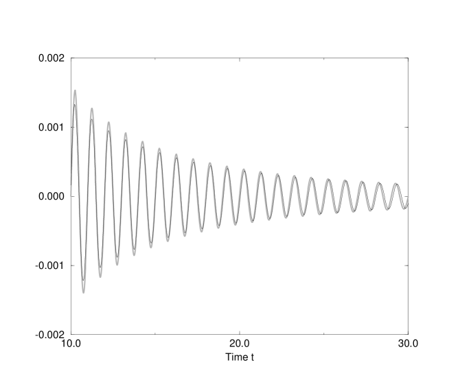
FIG. 2.: The comparison of Eq. (32) (gray line) to the numerical result (black line) with $k=m_{D}=2\pi$. The constant-amplitude oscillation has been subtracted.

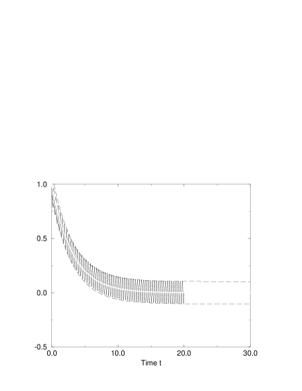
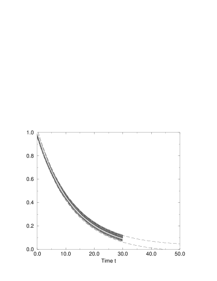
FIG. 3.: Results of the Landau damping simulations with $k=2\pi$ and $m_{D}=10\pi$ (left) and $m_{D}=20\pi$ (right). The white line is the predicted Landau damping rate $\gamma_{L}$ and the dashed lines show the envelope of the analytical result (36).

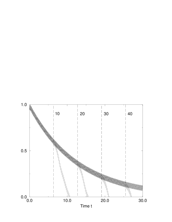
FIG. 4.: Landau damping simulations with $N_{\rm max}=10\ldots 40$ ($k=2\pi$, $m_{D}=20\pi$). The vertical dashed lines show the analytical prediction $t\approx 4N_{\rm max}/k$ for the time when the approximation should break down. The black curve is the result with $N_{\rm max}=200$ and the gray curves correspond to $N_{\rm max}=10,20,30,40$ from left to right.

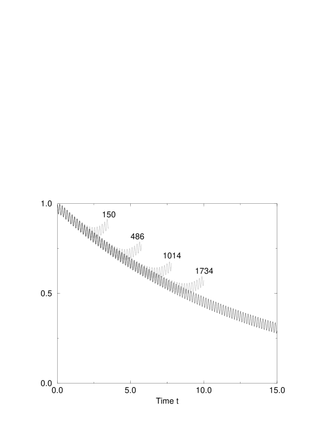
FIG. 5.: Landau damping simulations with $k=2\pi$, $m_{D}=20\pi$ in a formulation in which a large number of points on the unit sphere of velocities is used to approximate the integral. The values of $N_{v}$ were (from left to right) 2, 4, 6 and 8 and the corresponding numbers of degrees of freedom are shown in the plot.

TABLE I.: The approximate number of degrees of freedom needed in various approaches to simulate a mode with momentum $k$ reliably for time $t\gg 1/k$.

Approach	Degrees of freedom
Legendre polynomials	$4kt$
Spherical harmonics	$(kt)^{2}$
Discrete velocities	$\frac{24}{\pi^{2}}(kt)^{2}$

REFERENCES

- [1] K. Kajantie, M. Laine, K. Rummukainen, and M. Shaposhnikov, Nucl. Phys. B493, 413 (1997) [hep-lat/9612006].
- [2] P. Ginsparg, Nucl. Phys. B170, 388 (1980).
- [3] K. Kajantie, M. Laine, K. Rummukainen, and M. Shaposhnikov, Nucl. Phys. B458, 90 (1996) [hep-ph/9508379].
- [4] H. B. Nielsen and P. Olesen, Nucl. Phys. B61, 45 (1973).
- [5] T. W. B. Kibble, J. Phys. A9, 1387 (1976).
- [6] W. H. Zurek, Phys. Rept. 276, 177 (1996) [cond-mat/9607135].
- [7] G. Vincent, N. D. Antunes, and M. Hindmarsh, Phys. Rev. Lett. 80, 2277 (1998) [hep-ph/9708427].
- [8] D. Y. Grigoriev and V. A. Rubakov, Nucl. Phys. B299, 67 (1988).
- [9] V. A. Rubakov and M. E. Shaposhnikov, Usp. Fiz. Nauk 166, 493 (1996) [hep-ph/9603208].
- [10] D. Bödeker, L. McLerran, and A. Smilga, Phys. Rev. D52, 4675 (1995) [hep-th/9504123].
- [11] P. Arnold, Phys. Rev. D55, 7781 (1997) [hep-ph/9701393].
- [12] V. P. Silin, Sov. Phys. JETP 11, 1136 (1960).
- [13] R. D. Pisarski, Phys. Rev. Lett. 63, 1129 (1989); E. Braaten and R. D. Pisarski, Phys. Rev. D45, 1827 (1992).
- [14] V. P. Nair, Phys. Rev. D48, 3432 (1993) [hep-ph/9307326]; Phys. Rev. D50, 4201 (1994) [hep-th/9403146].
- [15] J. P. Blaizot and E. Iancu, Phys. Rev. Lett. 70, 3376 (1993) [hep-ph/9301236].
- [16] G. D. Moore, C. Hu, and B. Muller, Phys. Rev. D58, 045001 (1998) [hep-ph/9710436].
- [17] P. Dimopoulos, K. Farakos, and G. Koutsoumbas, Eur. Phys. J. C1, 711 (1998) [hep-lat/9703004].
- [18] K. Kajantie, M. Karjalainen, M. Laine, and J. Peisa, Nucl. Phys. B520, 345 (1998) [hep-lat/9711048].
- [19] K. Kajantie et al., Nucl. Phys. B, in press [hep-ph/9809334].
- [20] U. Kraemmer, A. K. Rebhan, and H. Schulz, Ann. Phys. 238, 286 (1995) [hep-ph/9403301].
- [21] E. Iancu, hep-ph/9710543; hep-ph/9809535.
- [22] C. R. Hu and B. Muller, Phys. Lett. B409, 377 (1997) [hep-ph/9611292].
- [23] D. Boyanovsky et al., Phys. Rev. D58, 125009 (1998) [hep-ph/9802370].
- [24] J.-P. Blaizot and E. Iancu, hep-ph/9903389.