Abstract

The procedures for studying a single narrow $s$-channel resonance or nearly degenerate resonances at a lepton collider, especially a muon collider, are discussed. In particular, we examine four methods for determining the parameters of a narrow $s$-channel resonance: scanning the resonance, measuring the convoluted cross section, measuring the Breit-Wigner area, and sitting on the resonance while varying the beam energy resolution. This latter procedure is new and appears to be potentially very powerful. Our focus is on computing the errors in resonance parameters resulting from uncertainty in the beam energy spread. Means for minimizing these errors are discussed. The discussion is applied to the examples of a light SM-Higgs, of the lightest pseudogoldstone boson of strong electroweak breaking, and of the two spin-1 resonances of the Degenerate BESS model (assuming that the beam energy spread is less than their mass splitting). We also examine the most effective procedures for nearly degenerate resonances, and apply these to the case of Degenerate BESS resonances with mass splitting of order the beam energy spread.

1 Introduction

The possibility of analyzing narrow $s$-channel resonances is considered to be one of the most important strengths of muon colliders, at present under consideration by different laboratories [1]. Most of the content of this note is indeed addressed to physics of particular relevance to future muon colliders (for general reviews see [2]). The importance of analyzing accurately an $s$-channel resonance at a lepton collider and the physical interest to be assigned to the extracted information are, of course, not new subjects. Much literature has in fact been devoted to the problem of the $Z$ resonance shape at electron-positron colliders and to the implications of its accurate measurement. Many of the special issues that arise when studying a narrow $s$-channel resonance, such as a light SM Higgs boson, have also been considered [3].

However, these latter studies assumed that the beam energy profile is perfectly known. If a resonance is so narrow that its width is smaller than or comparable to the beam energy spread, uncertainty in the beam’s energy profile can introduce substantial errors in the experimental determinations of the resonance parameters. One of the main goals of the present paper is to assess these errors. To this end, we shall present a detailed discussion of methods for studying a narrow $s$-channel resonance or systems of nearly degenerate resonances at a lepton collider, and consider applications to particular cases. We carefully analyze the errors in the measured resonance parameters (such as the total width and partial widths) that arise from the uncertainty in the energy spread of the beam. Procedures for reducing this source of errors are studied and experimental observables with minimal sensitivity to beam energy spread are emphasized. Our study will assume that the beam energy spread is independently measured, as will normally be possible. Expectations and procedures for this determination at a muon collider will be noted.

Although the parameters of a narrow $s$-channel resonance can be determined with minimal sensitivity to beam energy spread by measuring the total Breit-Wigner area, the peak total cross section and the cross sections in different final state channels, these measurements are not all easily performed with good statistical accuracy. Generally, a more effective method for determining resonance parameters is to scan the resonance using specific on- and off-resonance energy settings. In this paper, we also discuss the possibly superior new method introduced in Ref. [4] in which one operates the collider always with center of mass energy equal to the resonance mass but uses two different beam energy spreads: one smaller than the resonance width and one larger. All of these possibilities will be compared. The most immediate application is to the study of a light SM-Higgs, where, as already known [3, 5, 6], accurate measurements at a muon collider might make it possible to distinguish a standard model Higgs from the lightest Higgs of a supersymmetric model. We shall also analyze in detail resonant production of the lightest pseudogoldstone boson of dynamical electroweak symmetry breaking models. Following that, we consider two almost coincident vector resonances of the Degenerate BESS model [7] when their mass splitting is larger than the beam energy spread.

We shall then examine the case of two nearby resonances with mass splitting much smaller than their average mass, assuming that the energy spread of the beam is of the same order as the mass splitting. Different possible procedures for reducing the errors in the determination of the physical parameters will be examined. As an application we shall discuss such a situation in Degenerate BESS.

In Section 2 we present the analysis for a narrow resonance and in Section 3 the applications we have mentioned for this case. Section 4 gives the analysis for nearly degenerate resonances, and Section 5 a corresponding application.

2 Analysis for a narrow resonance

In this Section we will discuss several ways of determining the parameters of a narrow resonance at a lepton collider.

For a given decay channel, an $s$-channel resonance can be described by three parameters: the mass, the total width and the peak cross section. These quantities can only be accurately measured if the beam parameters are very well known. Measurement of the mass requires precise knowledge of the absolute energy value. Measurement of the width and cross section requires excellent knowledge of the energy spread of the beam and the ability to determine the difference between two beam energy settings with great precision.

All of these beam parameters must be known with extraordinary accuracy in order to study a very narrow resonance. For example, consider a light SM Higgs boson. In [3] it was found that the beam energy $E_{\rm beam}$ must be known to better than 1 part in $10^{6}$ and the beam energy spread $\Delta E_{\rm beam}$ must be smaller than 1 part in $10^{4}$ in order to scan the resonance and determine its width and other parameters. Below, we shall find that errors in these parameters due to uncertainty in $\Delta E_{\rm beam}$ will only be small compared to statistical errors associated with the measurements of a typical cross section (equivalent to a rate in a particular final state channel) if the error in the measurement of $\Delta E_{\rm beam}$ is smaller than $\sim 1\%$.

The independent measurement of $\Delta E_{\rm beam}$ can have both statistical and systematic error. Let us first consider the impact of statistical errors. We will argue that statistical uncertainties in $\Delta E_{\rm beam}$ (and also $E_{\rm beam}$ itself) should not be significant. Consider measurement of some resonance parameter $p$ through a series of observations over a large number ($S$) of spills. In a year of operation at a muon collider there will be something like $S=10^{8}$ spills. Each spill (i.e. each muon bunch) will contribute to the measurement of $p$, but the value of $p$ interpreted from the cross section $\sigma$ observed for a given spill will be uncertain by an amount $\delta p$. This uncertainty arises (a) because of the limited number of events $N_{i}$ accumulated during the spill and (b) due to uncertainties in $E_{\rm beam}$ and $\Delta E_{\rm beam}$ for that spill. We have, using the short hand notation of $E_{b}$ for $E_{\rm beam}$,

$$\left[\delta p\over p\right]_{i}=\left[{c^{2}\over N_{i}}+\left(a{\delta E_{b}\over E_{b}}\right)_{i}^{2}+\left(b{\delta\Delta E_{b}\over\Delta E_{b}}\right)_{i}^{2}\right]^{1/2}\,,$$ (1)

where $c={d\ln p\over d\ln\sigma}$, $a={d\ln p\over d\ln E_{b}}$ and $b={d\ln p\over d\ln\Delta E_{b}}$. $E_{b}$ and $\Delta E_{b}$ are measured by looking at oscillations in the spectra of the muon decay products arising due to spin precession of the muons in the bunch during the course of a very large number of turns around the ring. These measurements are completely independent of the measured rate(s) in question. The fractional statistical errors ${\delta E_{b}\over E_{b}}$ and ${\delta\Delta E_{b}\over\Delta E_{b}}$ for each spill are expected to be small as we shall summarize below. As a result, the contribution from the ${c^{2}\over N_{i}}$ term in Eq. (1) will normally be much larger than that from the $\delta E_{b}$ and $\delta\Delta E_{b}$ terms unless the coefficients $a$ and $b$ are very large. We will later learn that $a$ and $b$ will always be small under circumstances in which systematic errors in $E_{b}$ and $\Delta E_{b}$ do not badly distort the parameter measurement. To the extent that this is true, the statistical error $\delta p/p$ after a large number of spills, computed as

$${\delta p\over p}=\left[\sum_{i}{1\over\left({\delta p\over p}\right)_{i}^{2}}\right]^{-1/2}\,,$$ (2)

will be dominated by the usual $c/\sqrt{\sum_{i}N_{i}}$ term. Note that if this term were altogether absent, then ${\delta p\over p}$ would be proportional to $1/\sqrt{S}$ times the per spill error from $\delta E_{b}$ and $\delta\Delta E_{b}$. Thus, even if this latter were quite substantial, it would be strongly suppressed after accumulating data over $10^{8}$ spills.

Since $E_{\rm beam}$ and $\Delta E_{\rm beam}$ are expected to vary somewhat from spill to spill, what is important is the statistical error with which they can be measured in a given spill. This has been discussed in [8, 9, 10, 11]. Very roughly, the frequency of oscillation in the signal of secondary positrons from the muon decays (which signal is sensitive to the precession of the naturally-present polarization of the muons) determines $E_{\rm beam}$ and the decay with time of the oscillation signal amplitude determines $\Delta E_{\rm beam}/E_{\rm beam}$. At a resonance mass of $100~{}{\rm GeV}$,  a beam energy spread of $\Delta E_{\rm beam}/E_{\rm beam}\sim 3\times 10^{-5}$ can be achieved by an appropriate machine design while maintaining adequate yearly luminosity ($\geq 0.1~{}{\rm fb}^{-1}$). Further, in this case, for each muon spill (i.e. each muon bunch), one can determine the beam energy itself to 1 part in $10^{7}$ (5 keV) and measure the actual magnitude of $\Delta E_{\rm beam}/E_{\rm beam}$ with an accuracy of roughly $1.67\%$. For $\Delta E_{\rm beam}/E_{\rm beam}\sim 10^{-3}$, as might be useful for a much broader resonance than the SM Higgs boson and as would allow for substantially larger yearly integrated luminosity ($\geq 1~{}{\rm fb}^{-1}$), $E_{\rm beam}$ can be measured to 2 parts in $10^{6}$ (100 keV) and $\Delta E_{\rm beam}/E_{\rm beam}$ can be measured with an accuracy of roughly $0.2\%$. As described above, this level of statistical error for $E_{\rm beam}$ and $\Delta E_{\rm beam}/E_{\rm beam}$ will result in only a tiny $\delta p/p$ error for a given resonance parameter unless the coefficients $a$ and $b$ of Eq. (1) are very large. Thus, in what follows, we will analyze the parameter errors introduced by an uncertainty in $\Delta E_{\rm beam}/E_{\rm beam}$ that is assumed to be systematic in nature. The level of such uncertainty is not well understood at the moment. The energy spread will be affected by possible time dependence of other beam parameters, such as emmittance, by time-dependent backgrounds to the precession measurements, and by other sources of depolarization. Absent a detailed design for the machine and the polarimeter, [11] states that it is “quite certain” that the energy spread can be known with relative systematic error better than $\sim 1\%$, even if $\Delta E_{\rm beam}/E_{\rm beam}=3\cdot 10^{-5}$.

Given the precision with which the beam energy can be determined, it is clear that the mass of a resonance will be precisely known. We will not consider here the statistical errors in the measurements of the relevant cross sections, but these will later become important when choosing among the different procedures that we will discuss. Our main focus will be on the errors in the determination of branching ratios and total widths induced by a systematic uncertainty in the energy spread of the beam. Therefore, we will discuss the possibility of reducing such errors, and also discuss measurements which are independent of the energy spread. As already noted, these errors are expected to be important only when the width of the resonance is smaller than or comparable to the energy spread of the beam.

We assume that the resonance is well described by a Breit-Wigner shape. For a resonance $R$ of spin $j$ produced in the $s$-channel and decaying into a given final state $F$, one has

$$\sigma^{F}(E)=4\pi(2j+1)\frac{\Gamma(R\to\ell^{+}\ell^{-})\Gamma(R\to F)}{(E^{2}-M^{2})^{2}+M^{2}\Gamma^{2}}$$ (3)

where $M$ and $\Gamma$ are the mass and the width of the resonance, and $E=\sqrt{s}$. We will work in the narrow width approximation and therefore neglect the running of the width. We will consider also the total production cross section

$$\sigma(E)=4\pi(2j+1)\frac{\Gamma(R\to\ell^{+}\ell^{-})\Gamma}{(E^{2}-M^{2})^{2}+M^{2}\Gamma^{2}}$$ (4)

We assume that in the absence of bremsstrahlung the lepton beams have a Gaussian beam energy spread specified by $\Delta E_{\rm beam}/E_{\rm beam}=0.01\,R(\%)$, leading to a spread in the center of mass energy given by

$$\sigma_{E}={0.01\,R(\%)\over\sqrt{2}}\,E\sim 0.007\,R(\%)\,E\,.$$ (5)

In the absence of bremsstrahlung, the energy probability distribution $f(E)$ can be written in the scaling form

$$f(E)=\frac{1}{\sigma_{E}}g\left(\frac{E-E_{0}}{\sigma_{E}}\right)\,,$$ (6)

where $E_{0}$ is the central energy setting and

$$\int f(E)\,dE=1\,.$$ (7)

Accurate measurements of a narrow resonance require an accurate knowledge of both $\sigma_{E}$ and of the shape function $g$. We will explore the systematic uncertainties associated with errors in determining $\sigma_{E}$, assuming that the shape function $g$ is known to be of a Gaussian form.

After including bremsstrahlung (at an $e^{+}e^{-}$ collider, beamstrahlung must also be included) it is no longer possible to write the full energy distribution in a scaling form; bremsstrahlung has intrinsic knowledge of the mass of the lepton, which in leading order enters in the form $\log(E/m_{\ell})$. Since the bremsstrahlung distribution is completely known it may be convoluted with the scaling form of Eq. (6) to obtain a final energy distribution which depends upon both $\sigma_{E}$ and the (very accurately known) machine energy setting. Some useful figures illustrating the effects of bremsstrahlung at a muon collider are Figs. 30, 31 and 32 in Appendix A of [3]. One typically finds that the peak luminosity at the central beam energy, $E_{0}$, is reduced to about 60-80% of the value in the absence of bremsstrahlung, and that $d{\cal L}/dE$ falls below $10^{-3}\left.d{\cal L}/dE\right|_{E=E_{0}}$ at $E\sim 0.9E_{0}$. We will discuss results at a muon collider both before and after including bremsstrahlung, and show that the errors introduced by uncertainty in the beam energy spread can be very adequately assessed without including bremsstrahlung.

The measured cross sections are obtained from the convolution of the theoretical cross sections [see (3)] with the energy distribution:

$$\sigma_{c}^{F}(E)=4\pi(2j+1)\Gamma(R\to\ell^{+}\ell^{-})\Gamma(R\to F)h(\Gamma,\sigma_{E},E)$$ (8)

where

$$h(\Gamma,\sigma_{E},E)=\int\frac{f(E-E^{\prime})}{({E^{\prime}}^{2}-M^{2})^{2}+M^{2}\Gamma^{2}}dE^{\prime}$$ (9)

From these equations we can immediately draw two useful consequences:

• the ratio of $\sigma_{c}^{F}$ to the production cross section is given by

  $$\frac{\sigma_{c}^{F}}{\sigma_{c}}=B_{F},~{}~{}~{}B_{F}=B(R\to F)$$ (10)

  and does not depend on $\sigma_{E}$;

• due to the normalization condition (7), the integral of $\sigma_{c}^{F}$ is independent of $\sigma_{E}$

  $$\int\sigma_{c}^{F}(E)dE=\int\sigma^{F}(E)dE\,.$$ (11)

  Of course, one must be very certain that the integral over $E$ covers all of the resonance and all of the beam spread, including the low-energy bremsstrahlung tail.

Let us now consider the narrow resonance approximation. In this case, we can write

$$M^{2}\sigma^{F}(E)=\pi(2j+1)B_{\ell^{+}\ell^{-}}B_{F}\frac{\gamma^{2}}{x^{2}+\gamma^{2}/4}$$ (12)

where we have scaled the energy and the total width in terms of the energy spread evaluated at the peak (here we take $\sigma_{E}\approx\sigma_{M}$)

$$x=\frac{E-M}{\sigma_{M}},~{}~{}~{}~{}\gamma=\frac{\Gamma}{\sigma_{M}}$$ (13)

The convolution can also be written in terms of these variables, with the result (see Eq. (6))

In particular, for the production cross section, we get

$$M^{2}\sigma_{c}(E)=B_{\ell^{+}\ell^{-}}\,\Phi(x,\gamma)$$ (15)

Some simple results that are valid in the narrow resonance approximation are the following:

• If $\Gamma\gg\sigma_{M}$ (and $\Gamma$ is also large compared to bremsstrahlung energy spread), then

  $$\sigma_{c}(E)={4\pi B_{\ell^{+}\ell^{-}}\over M^{2}}{\Gamma^{2}M^{2}\over(E^{2}-M^{2})^{2}+\Gamma^{2}M^{2}}\,.$$ (16)

  A measurement of the peak cross section (summed over all final state modes) gives a direct measurement of $B_{\ell^{+}\ell^{-}}$. In addition, the resonance shape can be scanned by using a series of different energy settings for the machine and $\Gamma$ can then be determined.

• If $\Gamma\ll\sigma_{M}$, then

  $$\sigma_{c}(E)={4\pi B_{\ell^{+}\ell^{-}}\over M^{2}}{\Gamma\sqrt{\pi}\over 2\sqrt{2}\sigma_{M}}\exp\left[{-(E-M)^{2}\over 2\sigma_{M}^{2}}\right]\,,$$ (17)

  where we have assumed a Gaussian form for the beam energy spread. (We also neglected bremsstrahlung, but this could be easily included.) In this case, the peak cross section determines $B_{\ell^{+}\ell^{-}}\cdot\Gamma$ provided $\sigma_{M}$ is accurately known. $\sigma_{M}$ could in turn be measured by changing $E$ relative to $M$. However, statistical accuracy may be poor because cross sections are suppressed by $\Gamma/\sigma_{M}$ in comparison to those obtained if $\Gamma\geq\sigma_{M}$.

When scanning a resonance, the above limits make it clear that the cross section is largest and that systematic errors associated with $\sigma_{M}$ are smallest when $\sigma_{M}$ is as small compared to $\Gamma$ as possible. However, for a sufficiently narrow resonance, the luminosity reduction associated with achieving $\sigma_{M}$ values significantly smaller than $\Gamma$ is often so great that statistical uncertainties become large. Thus, we are often faced with a situation in which $\Gamma$ is comparable to or only a few times larger than $\sigma_{M}$. (For example, this will be the case when studying a light SM Higgs boson at a muon collider.) It is in this situation that systematic errors in the resonance parameters deriving from uncertainty in $\sigma_{M}$ can be enhanced.

We now discuss four ways of extracting $B_{\ell^{+}\ell^{-}}$, $B_{\ell^{+}\ell^{-}}B_{F}$ in a specific final state channel and $\Gamma$ from the data and assess the extent to which their determination will be influenced by uncertainty associated with an independent measurement of $\sigma_{M}$.

Table 1: Errors on $\Gamma$ and $B$ induced by $\Delta\sigma_{M}/\sigma_{M}=+0.05$ (upper lines) and $\Delta\sigma_{M}/\sigma_{M}=-0.05$ (lower lines) evaluated by choosing one observation at the peak and the other at $E-M=k\,\Gamma$, for $k=1,2,3$. Bremsstrahlung is neglected.

	$1\,\Gamma$		$2\,\Gamma$		$3\,\Gamma$
$\Gamma/\sigma_{M}$	$\Delta B/B$	$\Delta\Gamma/\Gamma$	$\Delta B/B$	$\Delta\Gamma/\Gamma$	$\Delta B/B$	$\Delta\Gamma/\Gamma$
1	${+0.220}$	${-0.205}$	${+0.171}$	${-0.160}$	${+0.114}$	${-0.101}$
	${-0.140}$	${+0.198}$	${-0.119}$	${+0.153}$	${-0.089}$	${+0.094}$
2	${+0.065}$	${-0.075}$	${+0.043}$	${-0.037}$	${+0.035}$	${-0.023}$
	${-0.053}$	${+0.072}$	${-0.039}$	${+0.035}$	${-0.033}$	${+0.023}$
3	${+0.031}$	${-0.036}$	${+0.023}$	${-0.017}$	${+0.022}$	${-0.013}$
	${-0.027}$	${+0.034}$	${-0.022}$	${+0.017}$	${-0.021}$	${+0.013}$
4	${+0.018}$	${-0.020}$	${+0.016}$	${-0.011}$	${+0.015}$	${-0.009}$
	${-0.017}$	${+0.019}$	${-0.015}$	${+0.010}$	${-0.014}$	${+0.009}$

Scan of the resonance - If $\Gamma\mathrel{\raise 1.29167pt\hbox{$>$\kern-7.5pt\lower 4.30554pt\hbox{$\sim$}}}\sigma_{M}$, one of the most direct ways to determine the parameters of an $s$-channel resonance is through a three-point scan [3]. In this method one measures the production cross section $\sigma_{c}$ at three different energies. However, the position of the peak is independent of the energy spread, and we do not expect that uncertainty in the latter will induce an error in the mass of the resonance (we have checked explicitly that this is indeed the case). Therefore we will assume in the following that the mass of the resonance is known with high accuracy, and, as a consequence, we will take into account only two scan points; one will be chosen at the peak and the other one off the peak. We will shortly discuss how the results depend on the position of this last point. The parameters $(B,\Gamma)$ are then extracted by a two parameter fit. Here, $B=B_{\ell^{+}\ell^{-}}$ if one is able to sum over all final state modes, and $B=B_{\ell^{+}\ell^{-}}B_{F}$ if one focuses on a particular final state. In principle this problem has a unique solution, by deconvoluting the observed cross section. However, the error in the determination of $\sigma_{M}$ (the energy spread at the peak of the resonance) induces an error on the determination of the parameters of the resonance. Assuming that the measured value of $\sigma_{c}$ at a given energy $E$ is given by $\sigma_{c}(E,B,\Gamma,\sigma_{M})$ (here again we use the narrow resonance approximation to put $\sigma_{E}\approx\sigma_{M}$), the changes in the values of $B$ and $\Gamma$ that result if $\sigma_{M}$ is shifted by an amount $\Delta\sigma_{M}$ can be evaluated through the equation

$$\sigma_{c}(E,B,\Gamma,\sigma_{M})=\sigma_{c}(E,B+\Delta B,\Gamma+\Delta\Gamma,\sigma_{M}+\Delta\sigma_{M})$$ (18)

or, from Eq. (15),

$$\Phi(x,\gamma)=\Phi(x+\Delta x,\gamma+\Delta\gamma)\left(1+\frac{\Delta B}{B}\right)$$ (19)

where

If we measure the cross section at two different energies, and assume that $\Delta\sigma_{M}$ is the same at these two nearby energies (as would be typical of a systematic error), we can easily employ Eq. (19) to determine the induced fractional shifts $\Delta\Gamma/\Gamma$ and $\Delta B/B$. We fix one of the two points at the peak ($x=0$), and we let the other one vary between $E-M=\Gamma$ and $E-M=3\Gamma$. The induced systematic errors are illustrated in a series of Tables. In Tables 1 and 2, we assume a Gaussian energy distribution without including bremsstrahlung and tabulate errors induced by $\Delta\sigma_{M}/\sigma_{M}=0.05$ and 0.01, respectively. As clear from Eq. (19), the fractional errors on $\Gamma$ and $B$ depend only on the $E-M$ choice and on the reduced width $\gamma$, but not on $B$.

Table 2: Same as Table 1 for $\Delta\sigma_{M}/\sigma_{M}=+0.01$ (upper lines) and $\Delta\sigma_{M}/\sigma_{M}=-0.01$ (lower lines).

	$1\,\Gamma$		$2\,\Gamma$		$3\,\Gamma$
$\Gamma/\sigma_{M}$	$\Delta B/B$	$\Delta\Gamma/\Gamma$	$\Delta B/B$	$\Delta\Gamma/\Gamma$	$\Delta B/B$	$\Delta\Gamma/\Gamma$
1	${+0.036}$	${-0.040}$	${+0.029}$	${-0.031}$	${+0.020}$	${-0.020}$
	${-0.033}$	${+0.040}$	${-0.027}$	${+0.031}$	${-0.019}$	${+0.019}$
2	${+0.012}$	${-0.015}$	${+0.008}$	${-0.007}$	${+0.007}$	${-0.004}$
	${-0.011}$	${+0.015}$	${-0.008}$	${+0.007}$	${-0.007}$	${+0.004}$
3	${+0.006}$	${-0.007}$	${+0.005}$	${-0.003}$	${+0.004}$	${-0.003}$
	${-0.006}$	${+0.007}$	${-0.004}$	${+0.003}$	${-0.004}$	${+0.003}$
4	${+0.004}$	${-0.004}$	${+0.003}$	${-0.002}$	${+0.003}$	${-0.002}$
	${-0.003}$	${+0.004}$	${-0.003}$	${+0.002}$	${-0.003}$	${+0.002}$

As expected from our earlier discussion, the fractional errors become smaller for larger $\Gamma/\sigma_{M}$. The fractional errors are also decreased by moving the second point of the scan away from the peak (see Tables 1 and 2). On the other hand the statistical errors for $\sigma_{c}$ are increasing as

$$\sigma_{c}(E)/\sigma_{c}(M)=\frac{\Phi(x,\gamma)}{\Phi(0,\gamma)}$$ (21)

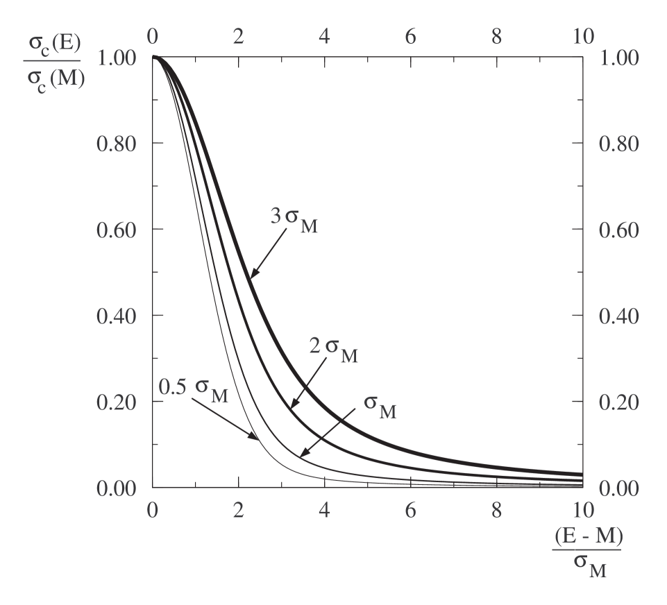
Figure 1: Plot of the ratio $\sigma_{c}(E)/\sigma_{c}(M)$ vs. $x=(E-M)/\sigma_{M}$, for $\Gamma=k\sigma_{M}$, with $k=0.5,1,2,3$.

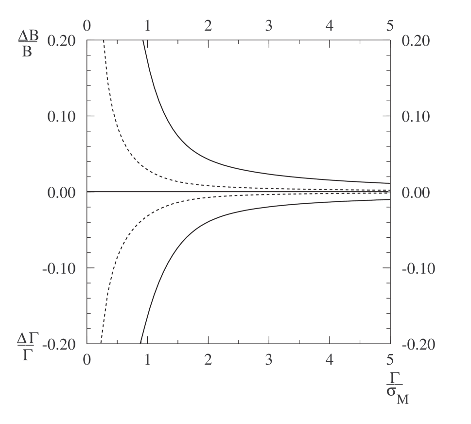
Figure 2: The fractional errors induced in $B$ and $\Gamma$ by $\Delta\sigma_{M}$ as functions of $\Gamma/\sigma_{M}$ when employing the three-point scan measurement ($E=M$, $E=M\pm 2\Gamma$); results are shown for $\Delta\sigma_{M}/\sigma_{M}=0.05$ (solid line) and $\Delta\sigma_{M}/\sigma_{M}=0.01$ (dashed line).

becomes smaller. (Due to presence of background, the decrease is not simply proportional to $\sqrt{\sigma_{c}(M)/\sigma_{c}(E)}$.) By fixing the amount of luminosity that one can safely lose without incurring substantial statistical error in $\sigma_{c}(E)$, and for a given ratio $\Gamma/\sigma_{M}$, one can, by looking at Fig. 1, fix the second scan point. For instance, for $\Gamma=2\sigma_{M}$, allowing for a loss in luminosity of 60%, we see that the point to be chosen is $x\approx 2$ corresponding to $E\approx M+\Gamma$. By choosing the second point of the scan at $E=M+2\Gamma$, the resulting behaviour of the systematic errors vs. $\gamma$ is illustrated in Fig. 2. For a given uncertainty on the energy spread the errors decrease for increasing $\gamma$. Therefore, as noted earlier, one should employ the smallest value of $\sigma_{M}$ consistent with having luminosity large enough to give small statistical $\sigma_{c}$ errors. For instance, at $\gamma=1$ the errors on the resonance parameters are of order $2.5\div 3.5$ times $\Delta\sigma_{M}/\sigma_{M}$, whereas for $\gamma=3$ they are down to $0.3\div 0.5$ times $\Delta\sigma_{M}/\sigma_{M}$.

Of course, a full study of the optimization of this procedure in a concrete case requires also taking into account the third scan point. In fact, one has the further freedom of moving the position of this point, with corresponding changes in the errors. One can show that by taking the third scan point in a symmetric position with respect to the other off-peak point, one gets the same errors shown in Tables 1 and 2 (in the absence of bremsstrahlung). By taking an asymmetric configuration the results are in between the ones obtained with the corresponding symmetric configurations. For instance, by taking one point at the peak, one at $E=M+2\Gamma$ and the third one at $E=M-\Gamma$, we find, for $\gamma=1$ and $\Delta\sigma_{M}/\sigma_{M}=0.05$, $\Delta\Gamma/\Gamma=-0.174$ and $\Delta B/B=+0.186$.

Table 3: Errors for $\Gamma$ and $B$ induced by $\Delta\sigma_{M}/\sigma_{M}=+0.05$ for no bremsstrahlung (first lines, from Table 1), and after including bremsstrahlung for $R=0.003\%$ (second lines), $R=0.03\%$ (third lines) and $R=0.1\%$ (fourth lines). The energy profile before bremsstrahlung is taken to be a Gaussian specified by the $\sigma_{M}$ corresponding to a given $R$ taking $M=100~{}{\rm GeV}$.

	$1\,\Gamma$		$2\,\Gamma$		$3\,\Gamma$
$\Gamma/\sigma_{M}$	$\Delta B/B$	$\Delta\Gamma/\Gamma$	$\Delta B/B$	$\Delta\Gamma/\Gamma$	$\Delta B/B$	$\Delta\Gamma/\Gamma$
1	${+0.22}$	${-0.21}$	${+0.17}$	${-0.16}$	${+0.11}$	${-0.10}$
	${+0.22}$	${-0.21}$	${+0.18}$	${-0.16}$	${+0.12}$	${-0.11}$
	${+0.22}$	${-0.21}$	${+0.18}$	${-0.16}$	${+0.12}$	${-0.11}$
	${+0.22}$	${-0.21}$	${+0.18}$	${-0.16}$	${+0.12}$	${-0.11}$
2	${+0.065}$	${-0.075}$	${+0.043}$	${-0.037}$	${+0.035}$	${-0.023}$
	${+0.067}$	${-0.078}$	${+0.046}$	${-0.044}$	${+0.040}$	${-0.032}$
	${+0.065}$	${-0.075}$	${+0.044}$	${-0.041}$	${+0.037}$	${-0.029}$
	${+0.067}$	${-0.077}$	${+0.045}$	${-0.042}$	${+0.039}$	${-0.031}$
3	${+0.031}$	${-0.036}$	${+0.023}$	${-0.017}$	${+0.022}$	${-0.013}$
	${+0.031}$	${-0.035}$	${+0.024}$	${-0.020}$	${+0.023}$	${-0.017}$
	${+0.031}$	${-0.037}$	${+0.024}$	${-0.020}$	${+0.023}$	${-0.017}$
	${+0.031}$	${-0.038}$	${+0.024}$	${-0.021}$	${+0.022}$	${-0.016}$
4	${+0.018}$	${-0.020}$	${+0.016}$	${-0.011}$	${+0.015}$	${-0.009}$
	${+0.019}$	${-0.022}$	${+0.017}$	${-0.013}$	${+0.015}$	${-0.011}$
	${+0.018}$	${-0.021}$	${+0.016}$	${-0.012}$	${+0.015}$	${-0.011}$
	${+0.018}$	${-0.020}$	${+0.015}$	${-0.012}$	${+0.015}$	${-0.011}$

Table 4: Errors for $\Gamma$ and $B$ expressed as $\Delta\Gamma/\Gamma=c_{\Gamma}\Delta\sigma_{M}/\sigma_{M}$ and $\Delta B/B=c_{B}\Delta\sigma_{M}/\sigma_{M}$ in the limit of small $\Delta\sigma_{M}/\sigma_{M}$. Same entry ordering and bremsstrahlung assumptions as in Table 3.

	$1\,\Gamma$		$2\,\Gamma$		$3\,\Gamma$
$\Gamma/\sigma_{M}$	$~{}~{}~{}c_{B}$	$~{}~{}~{}c_{\Gamma}$	$~{}~{}~{}c_{B}$	$~{}~{}~{}c_{\Gamma}$	$~{}~{}~{}c_{B}$	$~{}~{}~{}c_{\Gamma}$
1	3.4	$-$4.0	2.8	$-$3.1	2.0	$-$2.0
	3.6	$-$4.3	2.8	$-$3.2	2.1	$-$2.1
	3.2	$-$3.7	2.8	$-$3.2	2.1	$-$2.1
	3.4	$-$3.9	2.8	$-$3.2	2.1	$-$2.2
2	1.2	$-$1.5	0.81	$-$0.72	0.69	$-$0.45
	1.2	$-$1.5	0.85	$-$0.81	0.72	$-$0.59
	1.2	$-$1.5	0.86	$-$0.82	0.74	$-$0.61
	1.2	$-$1.5	0.85	$-$0.82	0.74	$-$0.61
3	0.58	$-$0.70	0.46	$-$0.34	0.43	$-$0.26
	0.62	$-$0.76	0.48	$-$0.40	0.43	$-$0.32
	0.60	$-$0.76	0.48	$-$0.42	0.46	$-$0.36
	0.57	$-$0.71	0.48	$-$0.42	0.44	$-$0.36
4	0.35	$-$0.40	0.31	$-$0.21	0.30	$-$0.17
	0.39	$-$0.45	0.30	$-$0.24	0.30	$-$0.26
	0.39	$-$0.43	0.32	$-$0.23	0.29	$-$0.23
	0.35	$-$0.40	0.29	$-$0.24	0.28	$-$0.20

Inclusion of bremsstrahlung might complicate the picture developed above, since the induced errors could, in principle, depend upon the resonance mass and the value of $R$, even when holding $\Gamma/\sigma_{M}$ and $(E-M)/\sigma_{M}$ fixed. To determine if the effects of bremsstrahlung are important for determining systematic errors coming from uncertainty in $\sigma_{M}$, we begin by considering again $\Delta\sigma_{M}/\sigma_{M}=+0.05$. We adopt $M=100~{}{\rm GeV}$ and consider $R=0.003\%$, $0.03\%$, and $0.1\%$ at a muon collider. The resulting errors are given in Table 3 in comparison to the no-bremsstrahlung results of the upper lines of Table 1. The induced errors computed including bremsstrahlung are quite independent of $R$ and (within the numerical errors of our programs) are essentially the same as those computed in the absence of bremsstrahlung. This can be further illustrated in the limit of very small $\Delta\sigma_{M}/\sigma_{M}$. In this limit, one can simply compute the errors induced in $B$ and $\Gamma$ by using a linear expansion of Eq. (18) and solving the resulting matrix equation. The results for $\Delta B/B$ and $\Delta\Gamma/\Gamma$ expressed as a coefficient times $\Delta\sigma_{M}/\sigma_{M}$ are given in Table 4 for four cases. The first case is that of no bremsstrahlung. (Note that for $\Delta\sigma_{M}/\sigma_{M}=\pm 0.01$ the errors predicted are quite close to those of Table 2.) The other three cases are for $M=100~{}{\rm GeV}$ and $R=0.003\%$, $0.03\%$, and $0.1\%$, including bremsstrahlung. Once again, we see that the error coefficients computed including bremsstrahlung do not depend much on $R$ and are essentially the same (within the numerical errors of our programs) as the error coefficients computed without including bremsstrahlung. Thus, in what follows we will discuss errors from $\Delta\sigma_{M}/\sigma_{M}$ without including the effects of bremsstrahlung. Once a particular resonance is discovered, the effects of bremsstrahlung upon the results presented here can be easily incorporated to whatever precision is required.

As regards $e^{+}e^{-}$ colliders, at which bremsstrahlung is a more substantial effect, a study (similar to that above for the $\mu^{+}\mu^{-}$ collider) shows that the Gaussian approximation for studying systematic errors from $\Delta\sigma_{M}$ is again reasonable. Although beamstrahlung is also important at an $e^{+}e^{-}$ collider, we did not study its effects. However, current $e^{+}e^{-}$ collider designs are such that the energy spreading from beamstrahlung is typically comparable to or smaller than that from bremsstrahlung.

An interesting general question regarding the scan procedure is how to optimize the choice of $\sigma_{M}$ relative to $\Gamma$ so as to minimize the net statistical plus systematic error. Let us consider using $k=1$ for the scan, assuming a resonance mass of $M=100~{}{\rm GeV}$ and that $\Delta\sigma_{M}/\sigma_{M}$ is small ($\mathrel{\raise 1.29167pt\hbox{$<$\kern-7.5pt\lower 4.30554pt\hbox{$\sim$}}}0.02$), so that the linear error expansion using coefficients $c_{\Gamma}$ and $c_{B}$ is valid. A very rough parameterization for the induced error in $\Gamma$ when $0.2\mathrel{\raise 1.29167pt\hbox{$<$\kern-7.5pt\lower 4.30554pt\hbox{$\sim$}}}\Gamma/\sigma_{M}\mathrel{\raise 1.29167pt\hbox{$<$\kern-7.5pt\lower 4.30554pt\hbox{$\sim$}}}3$ and $\Delta\sigma_{M}/\sigma_{M}\mathrel{\raise 1.29167pt\hbox{$<$\kern-7.5pt\lower 4.30554pt\hbox{$\sim$}}}0.02$ is

$${\Delta\Gamma\over\Gamma}\sim 3.3\left({\sigma_{M}\over\Gamma}\right)^{1.288}{\Delta\sigma_{M}\over\sigma_{M}}\,.$$ (22)

The optimal choice of $R$ for determining the parameters of a given resonance depends upon many factors: how the machine luminosity varies with $R$; the variation of $\Delta\sigma_{M}/\sigma_{M}$ with $R$; the variation of the $\Delta\sigma_{M}$-induced errors as a function of $R$; the magnitude of the resonance width (in particular, as compared to $\sigma_{M}$); and the size of backgrounds in the important final states to which the resonance decays. At a muon collider, $R$ in the range $0.1\%\div 0.15\%$ is the natural result and allows maximal luminosity. Increasing $R$ above this range does not result in significant luminosity increase; in contrast, the luminosity declines rapidly as $R$ is decreased below this range. A convenient parameterization for the luminosity of an $E=100~{}{\rm GeV}$ muon collider, valid for $0.003\%\mathrel{\raise 1.29167pt\hbox{$<$\kern-7.5pt\lower 4.30554pt\hbox{$\sim$}}}R\mathrel{\raise 1.29167pt\hbox{$<$\kern-7.5pt\lower 4.30554pt\hbox{$\sim$}}}0.12\%$, is: 

$$L_{\rm year}=1.2~{}{\rm fb}^{-1}\,\left({R\over 0.12\%}\right)^{0.67362}\,.$$ (23)

The specific coefficient in Eq. (23) represents the most pessimistic estimate for the instantaneous luminosities. On occasion we shall also discuss results assuming a factor of 10 larger coefficient, which we shall refer to as the optimistic luminosity estimate. We do not know what to expect for the variation of the systematic error in $\sigma_{M}$ as a function of $R$. In order to understand how the optimization might work, we have adopted on a purely adhoc basis a form that mimics the per-spill statistical error: 

$${\Delta\sigma_{M}\over\sigma_{M}}=2\cdot 10^{-3}\,\left({R\over 0.12\%}\right)^{-0.57477}\,.$$ (24)

This form corresponds to a decreasing fractional systematic error in $\sigma_{M}$ as $R$ increases, as seems a likely possibility. Finally, it is useful to recall the value of $\sigma_{M}$ as a function of $R$:

$$\sigma_{M}=86~{}{\rm MeV}\,{M\over 100~{}{\rm GeV}}\,\left({R\over 0.12\%}\right)\,.$$

For $R=0.003\%$, the smallest $R$ that is likely to be achievable, these quantities have the values $L_{\rm year}=0.1~{}{\rm fb}^{-1}$, ${\Delta\sigma_{M}/\sigma_{M}}=0.0167$, and $\sigma_{M}\sim 2~{}{\rm MeV}$ (for $M=100~{}{\rm GeV}$). The rough implications of these dependencies are as follows.

• For a broad resonance, defined as one with $\Gamma\gg 0.001M$, one should operate the muon collider at its natural $R$ value of order $0.12\%$. The $\Delta\sigma_{M}$-induced errors will be very tiny, both because $\Gamma/\sigma_{M}$ is very large and because $\Delta\sigma_{M}/\sigma_{M}$ should be small for such $R$. A precision scan of the resonance is readily possible in this case. Further, the resonance cross section is maximal for large $\Gamma/\sigma_{M}$ and both background and signal rates vary slowly as a function of $R$.

• For a resonance with $\Gamma<0.001M$, one will wish to reduce $R$ until $\Gamma\mathrel{\raise 1.29167pt\hbox{$>$\kern-7.5pt\lower 4.30554pt\hbox{$\sim$}}}\sigma_{M}$. The primary reasons to avoid $\Gamma<\sigma_{M}$ are to avoid the large $\Delta\sigma_{M}$-induced errors summarized above and to maintain adequate sensitivity to the resonance width. Keeping $\Gamma/\sigma_{M}>1$, one can combine the above formulae with the predicted variation of statistical error as a function of $R$ at fixed $L$ to determine the optimal $R$ choice. To illustrate, we will focus on the statistical error for $\Gamma$ obtained using the three-point scan with measurements at $E=M,M\pm 2\sigma_{M}$. If $\Gamma/\sigma_{M}$ is large (typically $>7\div 10$) the signal cross sections at the three scan points are roughly independent of $R$ (but only for $R$ values smaller than or not too much larger than that corresponding to $\sigma_{M}$). Since the background cross section is also independent of $R$, statistical errors would not vary much with $R$ if the total integrated luminosity is held fixed. More generally, one will find that, at fixed $L$, $\Delta\Gamma/\Gamma\propto R^{p}$ with $p>0$. (This is a very crude representation valid only for a limited range of $R$.) The exact rate of increase depends upon both $\Gamma/\sigma_{M}$ and the background level. Such cases will be discussed shortly. However, even if $p=0$, $\Delta\Gamma/\Gamma$ also varies as $1/\sqrt{L}$, where the available $L$ is given in Eq. (23). Defining $f\equiv R/0.003\%$, the net result is that we can write $(\Delta\Gamma/\Gamma)_{\rm stat.}=c_{\rm stat.}f^{p-0.337}$. Meanwhile, if we insert the expressions for $\sigma_{M}$ and $\Delta\sigma_{M}/\sigma_{M}$ in the expression for the $\Delta\sigma_{M}$-induced $\Delta\Gamma/\Gamma$, we find $(\Delta\Gamma/\Gamma)_{\rm syst.}=c_{\rm syst.}f^{0.713}$, where (for the $k=1$ three-point scan) $c_{\rm syst.}\sim 0.06\left({2~{}{\rm MeV}\over\Gamma}\right)^{1.288}$ if $M=100~{}{\rm GeV}$; we have normalized $\Gamma$ to the approximate width of a $100~{}{\rm GeV}$ SM Higgs boson. If $p-0.337<0$, as would apply for $p\sim 0$, then, if the statistical and systematic errors are added in quadrature, the opposite signs of their $f$ exponents means that there will be a minimum in the combined error as a function of $f$. If we use as a reference the value $f_{0}$ such that $c_{\rm stat.}=c_{\rm syst.}$, then one finds that the optimal $f$ is such that $f/f_{0}=R/R_{0}\sim 0.7$ when $p\sim 0$ (requiring $\Gamma/\sigma_{M}(R_{0})\gg 1$). In other words, one should choose a value of $R$ somewhat smaller than that value which would yield equal statistical and systematic errors.

  However, large $\Gamma/\sigma_{M}$ cannot be achieved for the very narrow Higgs and pseudogoldstone bosons discussed later in the paper. Even for the larger $M_{H}$ and $M_{P^{0}}$ values of possible interest for this optimization discussion, we have, at best, $\Gamma/\sigma_{M}(R=0.003\%)\sim 3\div 5$. Starting from $R=0.003\%$, one finds that, at fixed total $L$, $\Delta\Gamma/\Gamma$ increases quite rapidly with increasing $R$. As two examples, $\Gamma/\sigma_{M}(R=0.003\%)\sim 3$ ($\sim 5$) for a SM-like Higgs boson with $M_{H}\sim 140~{}{\rm GeV}$ ($\sim 150~{}{\rm GeV}$). In these two cases, $(\Delta\Gamma/\Gamma)_{\rm stat.}$ increases by a factor $\sim\sqrt{1}0$ ($\sim\sqrt{2}$) as $R$ increases from $0.003\%$ to $0.01\%$. Representing this increase using a power law (it is actually somewhat faster than a power law), we can roughly write $(\Delta\Gamma/\Gamma)_{\rm stat.}\sim cR^{p}$ at fixed $L$, with $p\sim 1$ ($p\sim 0.3$) for $M_{H}=140~{}{\rm GeV}$ ($M_{H}\sim 150~{}{\rm GeV}$). (Note that for $R$ above the $0.003\%$ to $0.01\%$ range, the $p$ values are much bigger.) From the analysis given in the preceding paragraph, we immediately see that if $p>0.337$, the best statistical and systematic errors will both be achieved by taking $R$ as small as possible. In the SM Higgs case, $\Gamma/\sigma_{M}>5$, corresponding to $M_{H}>150~{}{\rm GeV}$ would be required before $p<0.337$ and there could be some possible gain from increasing $R$. Similarly, in the case of the narrow pseudogoldstone boson $P^{0}$ it is only at the very largest $M_{P^{0}}=200~{}{\rm GeV}$ mass considered that $p$ falls just slightly below $0.337$. In practice, our a priori knowledge of $\Gamma$ (from the initial scan needed to pin down the precise location of the $H$ or $P^{0}$) will be too imprecise to allow for such optimization; one should plan on operating the machine at $R=0.003\%$ if initial information indicates that we are dealing with a Higgs or pseudogoldstone boson.

Measuring the on-peak cross sections for different $\sigma_{M}$ - In this technique [4] one presumes that $M$ is already quite well known and that one has in hand a rough idea of the size of $\Gamma$. (This is the likely result after the first rough scan used to locate the resonance.) One then operates the collider at $E=M$ for two different values of $\sigma_{M}$ (spending perhaps a year or two at each value). The results of Eqs. (16) and (17) show that if $\sigma_{M}^{\rm min}\ll\Gamma$ and $\sigma_{M}^{\rm max}\gg\Gamma$, then $\sigma_{c}(\sigma_{M}^{\rm min})/\sigma_{c}(\sigma_{M}^{\rm max})={2\sqrt{2}\sigma_{M}^{\rm max}\over\Gamma\sqrt{\pi}}$. The systematic error in $\Gamma$ is then given by $(\Delta\Gamma/\Gamma)_{\rm syst.}=\Delta\sigma_{M}^{\rm max}/\sigma_{M}^{\rm max}$. In practice, $\sigma_{M}^{\rm max}/\sigma_{M}^{\rm min}$ will be limited in size. If we define $\sigma_{M}^{\rm central}=\sqrt{\sigma_{M}^{\rm max}\sigma_{M}^{\rm min}}$ (the geometric mean value) and compute $r_{c}\equiv\sigma_{c}(\sigma_{M}^{\rm min})/\sigma_{c}(\sigma_{M}^{\rm max})=\Phi(0,\gamma_{\rm min})/\Phi(0,\gamma_{\rm max})$ (where $\gamma_{\rm max,min}=\Gamma/\sigma_{M}^{\rm max,min}$) as a function of $\Gamma$, our ability to measure $\Gamma$ in this way for any given value of $\sigma_{M}^{\rm max}/\sigma_{M}^{\rm min}$ is determined by the slope $|s|$ of $\ln[\Gamma/\sigma_{M}^{\rm central}]$ plotted as a function of $\ln[r_{c}]$. The relevant plot from Ref. [4] appears in Fig. 3. For a known $\sigma_{M}^{\rm central}$, the $|s|$ at any $\Gamma/\sigma_{M}^{\rm central}$ gives the relation $(\Delta\Gamma/\Gamma)_{\rm stat.}=|s|(\Delta r_{c}/r_{c})_{\rm stat.}$, where $\Delta r_{c}/r_{c}$ is computed by combining the fractional statistical errors for $\sigma_{c}(\sigma_{M}^{\rm min})$ and $\sigma_{c}(\sigma_{M}^{\rm max})$ in quadrature. The point at which the magnitude of the slope, $|s|$, is smallest indicates the point at which a given fractional statistical error in the cross section ratio will give the most accurate determination (as measured by fractional error) of $\Gamma/\sigma_{M}^{\rm central}$. We observe that $\Gamma/\sigma_{M}^{\rm central}\sim 2\div 3$ gives the smallest $|s|$ (and hence smallest statistical error), although $|s|$ at $\Gamma/\sigma_{M}^{\rm central}\sim 1$ is not that much larger. As expected, the larger $\sigma_{M}^{\rm max}/\sigma_{M}^{\rm min}$, the smaller $|s|$ at any given $\Gamma/\sigma_{M}^{\rm central}$. The systematic error in $\Gamma$ due to uncertainties in $\sigma_{M}^{\rm max}$ and $\sigma_{M}^{\rm min}$ is obtained from

$${\Phi\left(0,{\Gamma\over\sigma_{M}^{\rm min}}\right)\over\Phi\left(0,{\Gamma\over\sigma_{M}^{\rm max}}\right)}={\Phi\left(0,{\Gamma+\Delta\Gamma\over\sigma_{M}^{\rm min}+\Delta\sigma_{M}^{\rm min}}\right)\over\Phi\left(0,{\Gamma+\Delta\Gamma\over\sigma_{M}^{\rm max}+\Delta\sigma_{M}^{\rm max}}\right)}\,.$$ (25)

In most instances, the $\sigma_{M}^{\rm min}$ measurement is not very sensitive to the precise value of $\sigma_{M}^{\rm min}$, in which case the result is $(\Delta\Gamma/\Gamma)_{\rm syst.}=\Delta\sigma_{M}^{\rm max}/\sigma_{M}^{\rm max}$. More generally $(\Delta\Gamma/\Gamma)_{\rm syst.}=\Delta\sigma_{M}/\sigma_{M}$ to the extent that $\Delta\sigma_{M}/\sigma_{M}$ is the same at the different $\sigma_{M}$ settings (as might apply for systematic errors of a certain type). From this we see one clear advantage of this technique: the systematic error in $\Gamma$ due to systematic error in $\sigma_{M}$ does not increase with decreasing $\Gamma/\sigma_{M}^{\rm max,min}$. If statistical errors for measuring the two $\sigma_{c}$’s can be kept small, this is a clear advantage of the technique as compared to the scan technique in which small $\Gamma/\sigma_{M}$ leads to large $\Delta\sigma_{M}$-induced systematic error even if statistics are excellent for all measurements. We will shortly discuss issues related to statistical errors.

To continue our analysis of systematic errors, let us note that, in the limit of very high statistics for the cross section measurements (i.e. zero statistical error for $r_{c}$), precise values of both $\gamma_{\rm min}=\Gamma/\sigma_{M}^{\rm min}$ and $\gamma_{\rm max}=\Gamma/\sigma_{M}^{\rm max}$ are obtained by the above procedure. Further, $\sigma_{c}(\sigma_{M}^{\rm min})$ and $\sigma_{c}(\sigma_{M}^{\rm max})$ are given by $B\Phi(0,\gamma_{\rm min})$ and $B\Phi(0,\gamma_{\rm max})$, respectively, where $B$ stands for $B_{\ell^{+}\ell^{-}}$ or $B_{\ell^{+}\ell^{-}}B_{F}$, depending upon whether we are looking at the total rate or the rate in some particular final channel $F$. As a result, there is no systematic error in $B$ from uncertainty in $\sigma_{M}$, only statistical error associated with the number of events observed. This is another advantage of this technique.

Of course small systematic errors are not important if statistical errors for the technique are not also small. We summarize the considerations [4]. For the SM Higgs and the $P^{0}$ we found that it is best to use $\sigma_{M}^{\rm min}$ corresponding to $R=0.003\%$ and $\sigma_{M}^{\rm max}$ corresponding to $R=0.03\%$, so that $\sigma_{M}^{\rm central}$ corresponds to $R=0.003\%\times\sqrt{10}$. The parameterization for the variation of $L_{\rm year}$ given in Eq. (23) implies that $L_{\rm year}=0.1~{}{\rm fb}^{-1}$ ($0.47~{}{\rm fb}^{-1}$) for $R=0.003\%$ ($0.03\%$). If, for example, $\Gamma/\sigma_{M}^{\rm central}=1$, one finds $\sigma_{c}(\sigma_{M}^{\rm min})/\sigma_{c}(\sigma_{M}^{\rm max})=4.5$, implying that the signal rate $S(\sigma_{M})=L_{\rm year}(\sigma_{M})\sigma_{c}(\sigma_{M})$ is nearly the same for $\sigma_{M}^{\rm max}$ as for $\sigma_{M}^{\rm min}$. However, the background rate $B$ is proportional to $L$ and thus $B/S$ is a factor of 4.7 times larger at $\sigma_{M}^{\rm max}$ than at $\sigma_{M}^{\rm min}$. Consequently, the statistical error in the measurement of $\sigma_{c}(\sigma_{M}^{\rm max})$ will be worse than for $\sigma_{c}(\sigma_{M}^{\rm min})$ for the same $S$.  For a given running time at a given $\sigma_{M}$, one must compute the channel-by-channel $S$ and $B$ rates, compute the fractional error in $\sigma_{c}(\sigma_{M})$ for each channel, and then combine all channels to get the net $\sigma_{c}(\sigma_{M})$ error. This must be done for $\sigma_{M}=\sigma_{M}^{\rm min}$ and $\sigma_{M}=\sigma_{M}^{\rm max}$. One then computes the net $r_{c}$ and net $\sigma_{c}$ errors as:

The ratio of running times at $\sigma_{M}^{\rm min}$ vs. $\sigma_{M}^{\rm max}$ cannot be chosen so as to simultaneously minimize the net $\Delta\sigma_{c}/\sigma_{c}$ and $\Delta r_{c}/r_{c}$. The former is minimized by running only at $\sigma_{M}^{\rm min}$, while the latter is typically minimized for $t(\sigma_{M}^{\rm min})/t(\sigma_{M}^{\rm max})\mathrel{\raise 1.29167pt\hbox{$<$\kern-7.5pt\lower 4.30554pt\hbox{$\sim$}}}1$. For the SM Higgs, a good compromise is to take $t(\sigma_{M}^{\rm min})/t(\sigma_{M}^{\rm max})=1$. As demonstrated in the next section, it turns out that for both the $P^{0}$ and the SM Higgs boson, the ratio $L_{\rm year}(R=0.03\%)/L_{\rm year}(R=0.003\%)\sim 4.7$ and the predicted cross sections and backgrounds are such that this technique is very competitive with the scan technique as regards statistical errors for $\Gamma$.

Of course, for resonances (such as those of the Degenerate BESS model considered later) that have fairly large widths, the normal scan procedure can achieve superior results to the $r_{c}$-ratio technique. This is because there will be little sacrifice in luminosity associated with choosing an $R$ such that $\Gamma/\sigma_{M}$ is substantially larger than 1. Measurements on the wings of the resonance will have nearly the same statistical accuracy as measurements at the resonance peak.

Measurement of $\Gamma$ using the ratio of the $\ell^{+}\ell^{-}$ final state and total cross sections - First of all let us discuss the measurement of absolute and relative branching ratios. This is possible by simply measuring the cross sections in different final states, holding the energy fixed: $\sigma_{c}^{F_{1}}/\sigma_{c}^{F_{2}}=B_{F_{1}}/B_{F_{2}}$ and $\sigma_{c}^{F}/\sigma_{c}=B_{F}$. As apparent from Eq. (10), such cross section ratios do not depend on $\sigma_{M}$. Therefore, we can measure branching ratios and ratios of branching ratios with no systematic error induced by the energy spread. Of course, to measure $\sigma_{c}$, we must be able to sum over all final states for which $B_{F}$ is substantial, taking into account backgrounds and systematics associated with correctly determining the relative normalizations of different final states. This might not be easy, and could even be impossible if the resonance has some effectively invisible decays unless the branching ratio for invisible decays can be measured in a different experimental setting (in particular, one in which invisible decays can be effectively ‘tagged’ by producing the resonance in association with some other particle).

Given $B_{\ell^{+}\ell^{-}}$, the value of $\sigma_{c}$ and Eq. (15) can then be used to determine $\Gamma$ if $\sigma_{M}$ is known. The error on $\Gamma$ induced by uncertainty in $\sigma_{M}$, given the absence of systematic error in $B_{\ell^{+}\ell^{-}}$, is obtained from Eq. (19) with $\Delta B=0$,

$$\Phi(x,\gamma)=\Phi(x+\Delta x,\gamma+\Delta\gamma)\,.$$ (27)

If we measure $\sigma_{c}$ and $\sigma_{c}^{\ell^{+}\ell^{-}}$ at the resonance peak we have $\Delta x=0$ and Eq. (27) then requires $\Delta\gamma=0$; in turn,

$$\Delta\gamma=0\longrightarrow\frac{\Delta\Gamma}{\Gamma}=\frac{\Delta\sigma_{M}}{\sigma_{M}}\,.$$ (28)

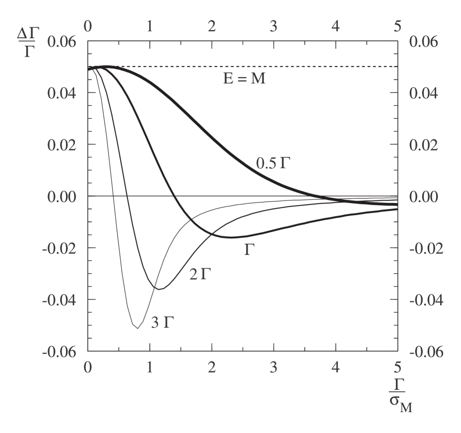
Figure 4: The fractional error induced in $\Gamma$ as a function of $\Gamma/\sigma_{M}$ for $E-M=k\Gamma$, with $k=0,1,2,3$, assuming a known value of $B_{\ell^{+}\ell^{-}}$ from the peak measurements of $\sigma_{c}$ and $\sigma_{c}^{\ell^{+}\ell^{-}}$. The value of $\Delta\sigma_{M}/\sigma_{M}$ is fixed at 0.05.

Therefore, the systematic error induced in $\Gamma$ does not depend on $\gamma$. On the other hand, if we move away from the peak, the situation changes drastically, as illustrated in Fig. 4 which gives $\Delta\Gamma/\Gamma$ vs. $\gamma$ for $\Delta\sigma_{M}/\sigma_{M}$ equal to 0.05. This figure can be trivially scaled for different values of $\Delta\sigma_{M}/\sigma_{M}$. We see that above $\gamma\approx 2$ the error decreases as one moves further away from the resonance peak. For values below $\gamma\approx 2$ the situation is more complicated, but for each choice of the energy there is a zero in the error.  Therefore, by opportunely choosing the energy of the measurement one could try to work in a region where the systematic error is very much reduced. For instance, if $\Gamma\approx 1.4\sigma_{M}$, by taking $E=M+\Gamma$, one has $\Delta\Gamma=0$. Notice that the locations of the zeroes do not depend on $\Delta\sigma_{M}$.

There are two potentially severe difficulties associated with this technique. First, in many instances the $\ell^{+}\ell^{-}$ decay mode has a small branching ratio. If the resulting event rate in the $\ell^{+}\ell^{-}$ final state is not large, the statistical error for $\sigma_{c}^{\ell^{+}\ell^{-}}$ will be large. Statistics for $E$ significantly different from $M$ (as required to take advantage of the zeroes discussed above) would be the first to become problematical. Second, we have already noted that measurement of $\sigma_{c}$ may be quite tricky. One must correctly normalize different final state channels relative to one another and assume that all final state channels with substantial branching ratio are visible. Regarding the latter, there is the alternative of measuring the branching ratio for invisible final states using other experimental situations/techniques and then making the appropriate correction to compute the full $\sigma_{c}$ given the contributions to $\sum_{F}\sigma_{c}^{F}$ that can be measured in the $s$-channel setting.

Of course, in some instances $B_{\ell^{+}\ell^{-}}$ will also be measured at other machines or via other processes. Also in this case, one can immediately determine $\Gamma$ given a measurement of $\sigma_{c}$. Alternatively, if $B_{F}$ is also known for some final state $F$ (as well as $B_{\ell^{+}\ell^{-}}$), $\sigma_{c}^{F}/(B_{\ell^{+}\ell^{-}}B_{F})$ will give a determination of $\Gamma$ with systematic uncertainty from $\Delta\sigma_{M}$ as described above.

Measurement of the Breit-Wigner area - As apparent from Eq. (11), the energy integral of the cross section does not depend on $\sigma_{M}$, and, in the narrow width approximation, is given by

$$\int\sigma_{c}(E)\,dE=4\pi^{2}(2j+1)\,\Gamma\cdot\,B_{\ell^{+}\ell^{-}}$$ (29)

Therefore, even if the energy spread is very poorly known, so long as it does not change as one scans over the resonance one could still measure the integral of the cross section, which is proportional to the product $\Gamma\cdot B_{\ell^{+}\ell^{-}}$, and obtain $B_{\ell^{+}\ell^{-}}$ from the ratio of the peak cross sections $\sigma_{c}^{\ell^{+}\ell^{-}}/\sigma_{c}$ (or, possibly, in another experimental setting). Of course, as discussed with regard to the previous procedure, the statistical error for $\sigma_{c}^{\ell^{+}\ell^{-}}$ might be large even when measured at the resonance peak. In addition, the event rate substantially off-resonance (as compared to both $\Gamma$ and $\sigma_{M}$) would be small (while typical backgrounds would be essentially constant). Thus, one can often only measure the cross section with good statistical accuracy over a limited portion of the full range.

If $\Gamma\gg\sigma_{M}$, and $\sigma_{M}$ is known ahead of time (via spin-precession measurements or the like), this fact will quickly become apparent after measuring the cross section at a few energy settings with $E-M\gg\sigma_{M}$. A reliable value for $\Gamma\cdot\,B_{\ell^{+}\ell^{-}}$ can normally be obtained so long as statistics are good at the peak. The procedure is that based on Eq. (16). One will measure $\sigma_{c}(E)$ for a set of points perhaps out to $E-M\sim\pm 2\Gamma$, and the remainder of the integral will be determined using the Breit-Wigner shape that would have been revealed by the measurements made. Sensitivity to $\sigma_{M}$ will be very minimal.

If $\sigma_{M}\gg\Gamma$, then the energy dependence of $\sigma_{c}(E)$ is determined by $\sigma_{M}$, see Eq. (17), or more generally by $g$ of Eq. (6) (bremsstrahlung should be included). Given a known value for $\sigma_{M}$ and a set of measured points, the remainder of the integral can be computed. However, statistical errors are likely to be quite large because the cross section is suppressed by the ratio $\Gamma/\sigma_{M}$.

Clearly, the most difficult case is that in which the resonance is very narrow and the smallest achievable $\sigma_{M}$ value is such that $\Gamma\sim\sigma_{M}$. Unless statistics remain good far off the peak, which is not likely, deconvolution of the effects of $\sigma_{M}$ and $\Gamma$ is required. The simplest deconvolution procedures for known $\sigma_{M}$ are the scan and ratio procedures outlined previously. Thus, if $\Gamma\sim\sigma_{M}$, the three-point scan technique and the technique of varying $\sigma_{M}$ while keeping $E=M$ are the most efficient for determining the parameters of an $s$-channel resonance so long as systematic uncertainty in the energy spread of the beam is smaller than $1\%\div 2\%$. (Of course, the appropriate strategy for exploring a resonance would be quite different if $\sigma_{M}$ is not independently measured with high statistical accuracy using the precession measurements.)

3 Applications

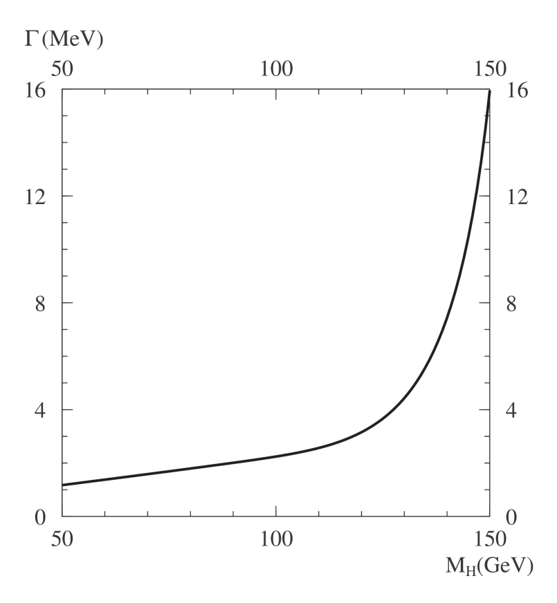
Figure 5: The total width of the SM-Higgs boson as a function of $M_{H}$.

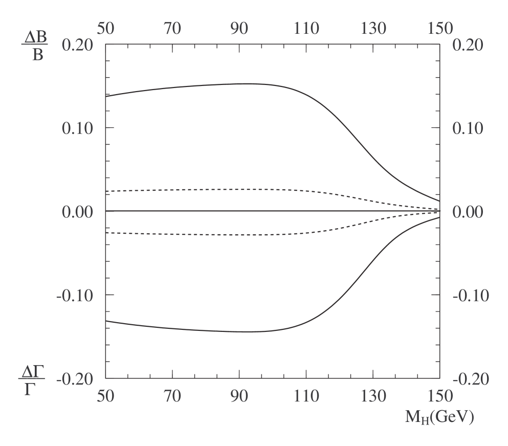
Figure 6: The $\Delta\sigma_{M}$-induced fractional errors in $B$ and $\Gamma$ as functions of $M_{H}$ assuming a three-point resonance scan ($E=M$, $E=M\pm 2\Gamma$); results are shown for $\Delta\sigma_{M}/\sigma_{M}=0.05$ (solid line) and $\Delta\sigma_{M}/\sigma_{M}=0.01$ (dashed line). The value of the beam resolution $R$ has been fixed to 0.003%.

SM-Higgs boson - In this Section we will apply the first two methods of Section 2 to the study of a light SM-Higgs boson. Consider first the three-point scan. By using the results of Fig. 2 one can easily determine the errors induced by the uncertainty in the energy spread as a function of the Higgs mass. For the evaluation of the Higgs width as a function of the mass, we make use of the expressions given in Ref. [12]. The decay channels we have considered are $b\bar{b}$, $\tau^{+}\tau^{-}$, $c\bar{c}$, $gg$ and $WW^{*}$, $ZZ^{*}$ (one of the two final bosons being virtual). The resulting total width is given in Fig. 5. We have considered the interval $50\leq M_{H}({\rm GeV})\leq 150$, but recall that, actually, there is an experimental lower bound at $90\%$ C.L. of about 90 GeV [13]. Below 110 GeV, the width of the Higgs increases approximately linearly with the mass (aside from logarithmic effects due to the running of the quark masses) which means that the ratio $\Gamma_{H}/\sigma_{M}$ is approximately constant. By choosing $R=0.003\%$ (see [5]) we get $\Gamma_{H}/\sigma_{M}\approx 1$. From Fig. 2, we see that the $\Delta\sigma_{M}$-induced errors in $B$ and in $\Gamma_{H}$ are about 15% and 2.5% for $\Delta\sigma_{M}/\sigma_{M}=0.05$ and 0.01, respectively, for a $k=2$ scan (as appropriate, given that $\Gamma_{H}\sim\sigma_{M}$, for comparing to the $E=M,~{}E=M\pm 2\sigma_{M}$ scan summarized below that was used to estimate statistical errors). Above 110 GeV, the systematic errors decrease rapidly due to the fast increase of the width. Fig. 6 summarizes the $\Delta B/B$ and $\Delta\Gamma_{H}/\Gamma_{H}$ fractional systematic errors as a function of $M_{H}$ for $R=0.003\%$ and $k=2$. Notice that, at least in the region up to 110 GeV, it will be mandatory to have values of $R$ of the order 0.003%. For instance, if we take $R=0.01\%$, corresponding to $\Gamma_{H}/\sigma_{M}\approx 0.3$ (for $50\leq M_{H}({\rm GeV})\leq 110$), the fractional $\Delta\sigma_{M}$-induced errors in $B$ and $\Gamma_{H}$ increase to about $14\%\div 16\%$ for $\Delta\sigma_{M}/\sigma_{M}=0.01$, as can be seen from the dashed line of Fig. 2.

Table 5: Percentage errors ($1\sigma$) for $\sigma_{c}B(H\to b\overline{b},WW^{\star},ZZ^{\star})$ (extracted from channel rates) and $\Gamma_{H}$ for $s$-channel Higgs production at the muon collider assuming beam energy resolution of $R=0.003\%$. Results are presented for two integrated four-year luminosities: $L=4~{}{\rm fb}^{-1}$ ($L=0.4~{}{\rm fb}^{-1}$). An optimized three-point scan is employed using measurements at $E=M_{H}$, $E=M_{H}+2\sigma_{M}$ and $E=M_{H}-2\sigma_{M}$, with luminosities of $L/5$, $2L/5$ and $2L/5$, respectively. [For the cross section measurements, this is equivalent to $L\sim 2~{}{\rm fb}^{-1}$ ($L=0.2~{}{\rm fb}^{-1}$) at the $E=M_{H}$ peak]. This table is taken from Ref. [5]. Efficiencies and cuts are those employed in [3]. The effects of bremsstrahlung are included.

Quantity	Errors
Mass (GeV)	80	$M_{Z}$	100	110
$\sigma_{c}B(b\overline{b})$	$0.8\%(2.4\%)$	$7\%(21\%)$	$1.3\%(4\%)$	$1\%(3\%)$
$\sigma_{c}B(WW^{\star})$	$-$	$-$	$10\%(32\%)$	$5\%(15\%)$
$\sigma_{c}B(ZZ^{\star})$	$-$	$-$	$-$	$62\%(190\%)$
$\Gamma_{H}$	$3\%(10\%)$	$25\%(78\%)$	$10\%(30\%)$	$5\%(16\%)$
Mass (GeV)	120	130	140	150
$\sigma_{c}B(b\overline{b})$	$1\%(3\%)$	$1.5\%(5\%)$	$3\%(9\%)$	$9\%(28\%)$
$\sigma_{c}B(WW^{\star})$	$3\%(10\%)$	$2.5\%(8\%)$	$2.3\%(7\%)$	$3\%(9\%)$
$\sigma_{c}B(ZZ^{\star})$	$16\%(50\%)$	$10\%(30\%)$	$8\%(26\%)$	$11\%(34\%)$
$\Gamma_{H}$	$5\%(16\%)$	$6\%(18\%)$	$9\%(29\%)$	$34\%(105\%)$

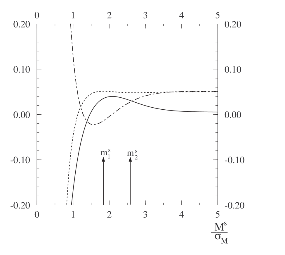
Figure 13: The fractional errors in the partial widths, $\Delta\Gamma(R_{i}\to\ell^{+}\ell^{-})/\Gamma(R_{i}\to\ell^{+}\ell^{-})$, $i=1,2$ (dashed and dot-dashed lines respectively), and in the mass splitting, $\Delta M^{s}/M^{s}$ (continuous line), induced by an energy spread uncertainty of $\Delta\sigma_{M}/\sigma_{M}=0.05$, as a function of $m^{s}$ for $a=\Gamma(R_{2}\to\ell^{+}\ell^{-})/\Gamma(R_{1}\to\ell^{+}\ell^{-})=2$. The input cross section measurements are at $x_{max}$, see Eq. (46), $x=0.1$ and $x=0.2$.

It is interesting to compare these systematic errors to the statistical errors. The analysis at a muon collider done in Ref. [5] gives statistical errors for a three-point scan using scan points at $E=M,~{}E=M\pm 2\sigma_{M}$ and $R=0.003\%$, assuming $L=4~{}{\rm fb}^{-1}$ or $L=0.4~{}{\rm fb}^{-1}$ total accumulated luminosity (corresponding to 4 years of operation for optimistic or pessimistic, respectively, instantaneous luminosity). The results of that analysis are summarized in Table 5. Except for $M_{H}\sim M_{Z}$, the $L=4~{}{\rm fb}^{-1}$ statistical error for measuring the total width would be of order $3\%\div 10\%$ when $80\leq M_{H}\leq 140~{}{\rm GeV}$. Therefore, to avoid contaminating this high precision measurement error with systematic uncertainty from $\Delta\sigma_{M}$ we will certainly want to have $\Delta\sigma_{M}/\sigma_{M}\mathrel{\raise 1.29167pt\hbox{$<$\kern-7.5pt\lower 4.30554pt\hbox{$\sim$}}}1\%$. If one adopts the $L=0.4~{}{\rm fb}^{-1}$ luminosity assumption (the benchmark value of Refs. [10, 11]), and if $m_{H}<130~{}{\rm GeV}$ and not near $M_{Z}$, the statistical measurement error for $\Gamma_{H}$ is in the 10% to 20% range. This means that $\Delta\sigma_{M}/\sigma_{M}$ as large as $5\%$ would be very undesirable. Finally, we re-emphasize the fact that performing the scan using larger $R$ than $R=0.003\%$ leads to larger statistical errors until $M_{H}$ approaches the $WW$ decay threshold and $\Gamma_{H}/\sigma_{M}(R=0.003\%)>5$. For lower $M_{H}$, the $R=0.003\%$ results are the best that can be achieved despite the smaller luminosity at $R=0.003\%$ as compared to higher $R$ values. For example, the error in $\Gamma_{H}$ for a given luminosity using $R=0.01\%$ can be read off from Fig. 13 of [3]. One finds that $L(R=0.01\%)/L(R=0.003\%)=20,10,2$ is required in order that the $\Gamma_{H}$ statistical errors for $R=0.01\%$ be equal to those for $R=0.003\%$ at $M_{H}=130,140,150~{}{\rm GeV}$, respectively. Existing machine designs are such that $L_{\rm year}(R=0.01\%)/L_{\rm year}(R=0.003\%)=0.22~{}{\rm fb}^{-1}/0.1~{}{\rm fb}^{-1}=2.2$. Thus, increasing $R$ would not improve the scan-procedure statistical errors until $M_{H}>150~{}{\rm GeV}$. In addition, $\Delta\sigma_{M}$-induced systematic errors always rise rapidly with increasing $R$. For $M_{H}\leq 150~{}{\rm GeV}$, one should employ the smallest value of $R$ possible.

Table 6: Percentage errors ($1\sigma$) for $\sigma_{c}B(H\to b\overline{b},WW^{\star},ZZ^{\star})$ (extracted from channel rates) and $\Gamma_{H}$ for $s$-channel Higgs production at the muon collider. Operation at $E=M_{H}$ is assumed and the $r_{c}$-ratio technique is used for determining $\Gamma_{H}$. Results are presented assuming accumulated luminosities of $L=2~{}{\rm fb}^{-1}$ ($L=0.2~{}{\rm fb}^{-1}$) at $R=0.003\%$ and $L=9.4~{}{\rm fb}^{-1}$ ($L=0.94~{}{\rm fb}^{-1}$) at $R=0.03\%$, corresponding to roughly two years of running at each $R$ for optimistic (pessimistic) instantaneous luminosity assumptions. Efficiencies and cuts employed appear in [3]. The effects of bremsstrahlung are included.

Quantity	Errors
Mass (GeV)	80	$M_{Z}$	100	110
$\sigma_{c}B(b\overline{b})$	$0.7\%(2.2\%)$	$6.3\%(20\%)$	$1.2\%(3.8\%)$	$0.9\%(2.8\%)$
$\sigma_{c}B(WW^{\star})$	$-$	$-$	$8.2\%(26\%)$	$3.8\%(12\%)$
$\sigma_{c}B(ZZ^{\star})$	$-$	$-$	$-$	$60\%(190\%)$
$\Gamma_{H}$	$6\%(19\%)$	$63\%(200\%)$	$14\%(45\%)$	$8\%(25\%)$
Mass (GeV)	120	130	140	150
$\sigma_{c}B(b\overline{b})$	$0.9\%(2.8\%)$	$1.4\%(4.4\%)$	$2.4\%(7.6\%)$	$6.6\%(21\%)$
$\sigma_{c}B(WW^{\star})$	$2.4\%(7.7\%)$	$1.8\%(5.7\%)$	$1.6\%(5.0\%)$	$1.8\%(5.6\%)$
$\sigma_{c}B(ZZ^{\star})$	$15\%(46\%)$	$7.9\%(25\%)$	$6.3\%(20\%)$	$7.0\%(22\%)$
$\Gamma_{H}$	$6.3\%(20\%)$	$6\%(19\%)$	$5.4\%(17\%)$	$4.7\%(18\%)$

Let us now compare to the $r_{c}$-ratio technique. We employ the same total of 4 years of operation as considered for the three-point scan, but always with $E=M_{H}$. As noted earlier, a good sharing of time is to devote two years to running at $R=0.003\%$, accumulating $L=2~{}{\rm fb}^{-1}$ ($L=0.2~{}{\rm fb}^{-1}$) for optimistic (pessimistic) instantaneous luminosity, and a second two years to running at $R=0.03\%$, corresponding to [using the luminosity scaling law of Eq. (23)] $L=9.4~{}{\rm fb}^{-1}$ ($L=0.94~{}{\rm fb}^{-1}$) of accumulated luminosity. For $R=0.03\%$, $\Gamma_{H}/\sigma_{M}^{\rm max}\sim 0.1$ and, as noted earlier, each $\sigma_{c}B_{F}$ cross section is decreased by almost the same factor by which the luminosity has increased, leaving the number of signal events unchanged. However, the background is increased by a factor of 4.7. A complete calculation is required. This was performed in [4]. The various $\sigma_{c}B_{F}$ statistical errors are summarized in Table 6 along with the $\Delta\Gamma_{H}/\Gamma_{H}$ statistical error computed by combining all the listed final state channels and following the procedure of Eq. (LABEL:sigcerror). We observe that the ratio technique becomes superior to the scan technique for the larger $M_{H}$ values ($M_{H}>130~{}{\rm GeV}$). This is correlated with the fact that $\Gamma_{H}/\sigma_{M}^{\rm min}$ (where $\sigma_{M}^{\rm min}$ is that for $R=0.003\%$) becomes substantially larger than 1 for such $M_{H}$. In particular, for larger $M_{H}$, $\Gamma_{H}/\sigma_{M}^{\rm central}$ is in a range such that $|s|$ and, consequently, the error in $\Gamma_{H}$ will be minimal. Thus, the two techniques are actually quite complementary — by employing the best of the two procedures, a very reasonable determination of $\Gamma_{H}$ and very precise determinations of the larger channel rates will be possible for all $M_{H}$ below $2M_{W}$.

Finally, we again note that the $r_{c}$-ratio technique has the advantage that the $\Delta\sigma_{M}$-induced systematic error in $\Gamma_{H}$ is equal to $\Delta\sigma_{M}/\sigma_{M}$ and will, therefore, be smaller by a factor of about 2.5 (if $M_{H}\leq 120~{}{\rm GeV}$) for the $r_{c}$-ratio technique than for the scan technique and that there is no $\Delta\sigma_{M}$-induced systematic error in the $B_{\ell^{+}\ell^{-}}B_{F}$ determinations. Thus, although the statistical errors for the $r_{c}$-ratio procedure are larger than for the scan procedure when $M_{H}<130~{}{\rm GeV}$, if the fractional error in $\sigma_{M}$ is substantially larger than $0.01$, the $r_{c}$-ratio could have net overall (statistical plus systematic) error that is smaller than the scan technique down to $M_{H}$ values significantly below $130~{}{\rm GeV}$.

The lightest PNGB - The $s$-channel production of the lightest neutral pseudo-Nambu-Goldstone boson (PNGB) ($P^{0}$), present in models of dynamical breaking of the electroweak symmetry which have a chiral symmetry larger than $SU(2)\times SU(2)$, has recently been explored [14, 15]. In the broad class of models considered in [14], the $P^{0}$ is of particular interest because it contains only down-type techniquarks (and charged technileptons) and thus has a mass scale that is most naturally set by the mass of the $b$-quark. Other color-singlet PNGB’s will have masses most naturally set by $m_{t}$, while color non-singlet PNGB’s will generally be even heavier. The $M_{P^{0}}$ mass range, that is typically suggested by technicolor models [16], is $10~{}{\rm GeV}<M_{P^{0}}<200~{}{\rm GeV}$.

Discovery of the $P^{0}$ in the $gg\to P^{0}\to\gamma\gamma$ mode at the Tevatron Run II and at the LHC will almost certainly be possible unless its mass is either very small ($\mathrel{\raise 1.29167pt\hbox{$<$\kern-7.5pt\lower 4.30554pt\hbox{$\sim$}}}30~{}{\rm GeV}$?) or very large ($\mathrel{\raise 1.29167pt\hbox{$>$\kern-7.5pt\lower 4.30554pt\hbox{$\sim$}}}200~{}{\rm GeV}$?), where the question marks are related to uncertainties in backgrounds in the inclusive $\gamma\gamma$ channel. Run I data at Tevatron can already be used to exclude a $P^{0}$ in the $50-200~{}{\rm GeV}$ mass range for a number of technicolors $N_{TC}>12-16$. In contrast, an $e^{+}e^{-}$ collider, while able to discover the $P^{0}$ via $e^{+}e^{-}\to\gamma P^{0}$, so long as $M_{P^{0}}$ is not close to $M_{Z}$, is unlikely (unless the TESLA $500~{}{\rm fb}^{-1}$ per year option is built or $N_{TC}$ is very large) to be able to determine the rates for individual $\gamma F$ final states ($F=b\overline{b},\tau^{+}\tau^{-},gg$ being the dominant $P^{0}$ decay modes) with sufficient accuracy such as to yield more than very rough indications about the parameters of the technicolor model. The $\gamma\gamma$ collider mode of operation at an $e^{+}e^{-}$ collider would allow one to discover and study the $P^{0}$ with greater precision.

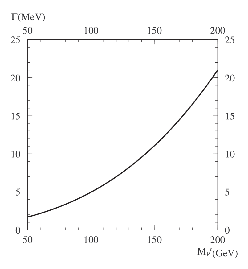
Figure 7: The total width of the lightest PNGB $P^{0}$ as a function of $M_{P^{0}}$ (for the choice of model parameters given in Ref. [14]).

A $\mu^{+}\mu^{-}$ collider would play a very special role with regard to determining key properties of the $P^{0}$. In particular, the $P^{0}$, being comprised of $D\overline{D}$ and $E\overline{E}$ techniquarks, will naturally have couplings to the down-type quarks and charged leptons of the SM. Thus, $s$-channel production ($\mu^{+}\mu^{-}\to P^{0}$) is predicted to have a substantial rate for $\sqrt{s}\sim M_{P^{0}}$. Because the $P^{0}$ has a very narrow width (see Fig. 7), not much larger than that of a SM-Higgs boson of the same mass, in order to maximize this rate it is important that one operates the $\mu^{+}\mu^{-}$ collider so as to have extremely small beam energy spread, $R=0.003\%$. For such an $R$, the resolution in $E=\sqrt{s}$ of the muon collider, $\sigma_{E}$, is of order $\sigma_{E}\sim 1~{}{\rm MeV}(E/50~{}{\rm GeV})$, whereas the $P^{0}$ width, $\Gamma_{P^{0}}$, varies from $2~{}{\rm MeV}$ to $20~{}{\rm MeV}$ as $M_{P^{0}}$ ranges from $50~{}{\rm GeV}$ up to $200~{}{\rm GeV}$ (small differences with respect to [14] come from running fermion masses). Thus, $\sigma_{E}<\Gamma_{P^{0}}$ is possible and leads to very high $P^{0}$ production rates for typical $\mu^{+}\mu^{-}\to P^{0}$ coupling strength.

Assuming that the $P^{0}$ is discovered at the Tevatron, the LHC or (as might be the only possibility if $M_{P^{0}}$ is very small) at an $e^{+}e^{-}$ collider (possibly operating in the $\gamma\gamma$ collider mode), the $\mu^{+}\mu^{-}$ collider could quickly (in less than a year) scan the mass range indicated by the previous discovery (for the expected uncertainty in the mass determination) and center on $\sqrt{s}\simeq M_{P^{0}}$ to within $<\sigma_{M}$. A first very rough estimate of $\Gamma_{P^{0}}$ would also emerge from this initial scan. One would then proceed with a dedicated study of the $P^{0}$. One technique would be to use the optimal three-point scan [14] of the $P^{0}$ resonance (with measurements at $E=M_{P^{0}}$ and $E=M_{P^{0}}\pm 2\sigma_{M}$ using $R=0.003\%$). The three-point scan would determine with high statistical precision all the $\mu^{+}\mu^{-}\to P^{0}\to F$ channel rates and give a reasonably accurate measurement of the total width $\Gamma_{P^{0}}$. For the particular technicolor model parameters analysed in [14], 4 years of the pessimistic yearly luminosity ($L_{\rm year}=0.1~{}{\rm fb}^{-1}$) devoted to the scan yields the results presented in Fig. 19 of [14].  Sample statistical errors for $\sigma_{c}B(P^{0}\to{\rm all})$ and $\Gamma_{P^{0}}$ taken from this figure at $M_{P^{0}}=60~{}{\rm GeV}$, $80~{}{\rm GeV}$, $M_{Z}$, $110~{}{\rm GeV}$, $150~{}{\rm GeV}$ and $200~{}{\rm GeV}$ are given in Table 7.

Table 7: Fractional statistical errors ($1\sigma$) for $\sigma_{c}B(P^{0}\to{\rm all})$ (combining $b\bar{b}$, $\tau^{+}\tau^{-}$, $c\bar{c}$ and $gg$ tagged-channel rates — see [14]) and $\Gamma_{P^{0}}$ for $s$-channel $P^{0}$ production at the muon collider. We compare results for an $R=0.003\%$ three-point scan with total integrated luminosity of $L=0.4~{}{\rm fb}^{-1}$ (corresponding to four years of running at pessimistic luminosity, with distribution $L/5$ at $E=M_{P^{0}}$, $2L/5$ at $E=M_{P^{0}}+2\sigma_{M}$ and $2L/5$ at $E=M_{P^{0}}-2\sigma_{M}$) to results obtained using the $r_{c}$-ratio technique assuming accumulated luminosities at $E=M_{P^{0}}$ of $L=0.2f~{}{\rm fb}^{-1}$ at $R=0.003\%$ and $L=0.94(2-f)~{}{\rm fb}^{-1}$ at $R=0.03\%$ (corresponding to roughly $2f$ years of running at $R=0.003\%$ and $(4-2f)$ years of running at $R=0.03\%$ for pessimistic instantaneous luminosity assumptions). $f$ (tabulated below) is chosen to minimize the error in $\Gamma_{P^{0}}$. We employ the efficiencies, cuts and tagging procedures described in [14]. The effects of bremsstrahlung are included.

Quantity	Errors for the scan procedure
Mass (GeV)	60	80	$M_{Z}$	110	150	200
$\sigma_{c}B$	0.0029	0.0054	0.043	0.0093	0.012	0.018
$\Gamma_{P^{0}}$	0.014	0.029	0.25	0.042	0.052	0.10
Quantity	Errors for the $r_{c}$-ratio procedure
Mass (GeV)	60	80	$M_{Z}$	110	150	200
$f$	0.8	0.7	0.6	0.8	0.9	1.0
$\sigma_{c}B$	0.0029	0.0062	0.055	0.010	0.011	0.016
$\Gamma_{P^{0}}$	0.014	0.028	0.24	0.041	0.039	0.053

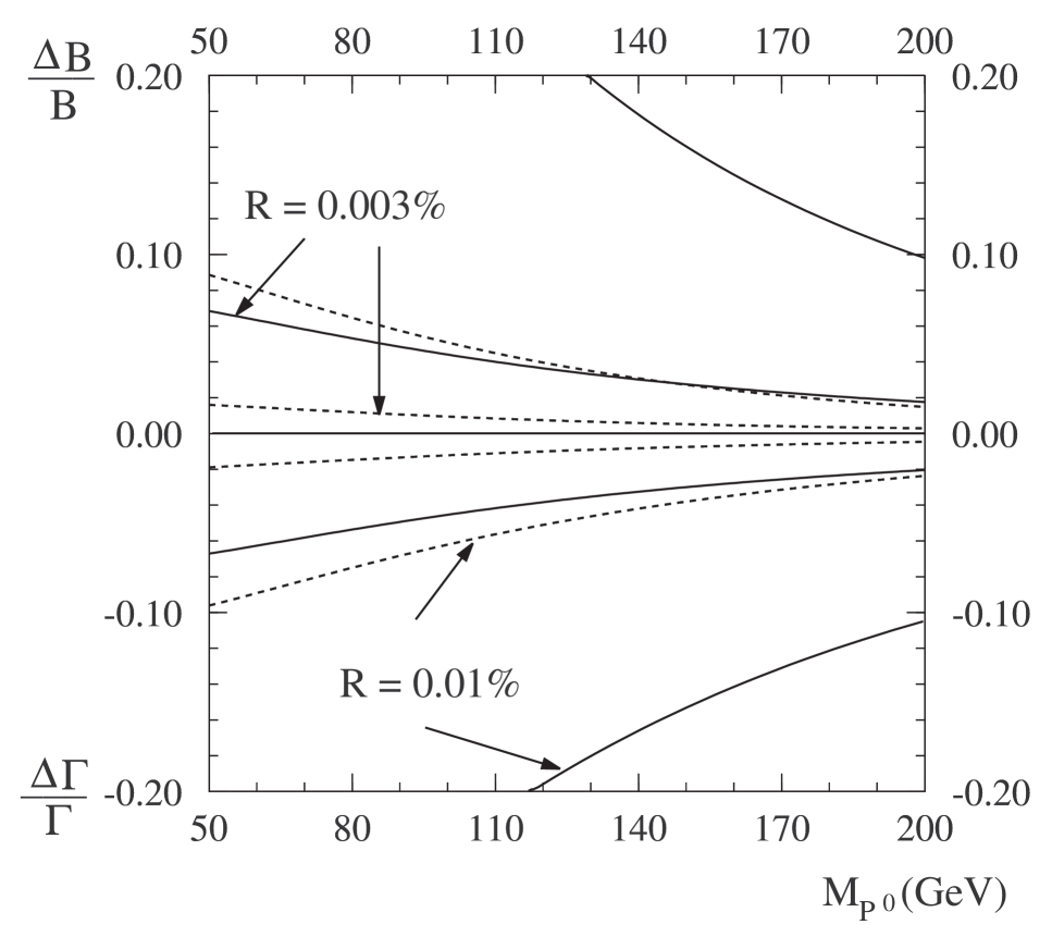
Figure 8: The $\Delta\sigma_{M}$-induced fractional errors in $B$ and $\Gamma=\Gamma_{P^{0}}$ as functions of $M_{P^{0}}$ assuming a three-point resonance scan ($E=M$, $E=M\pm 2\sigma_{M}$); results are shown for $\Delta\sigma_{M}/\sigma_{M}=0.05$ (solid line) and $\Delta\sigma_{M}/\sigma_{M}=0.01$ (dashed line), and for $R=0.003\%$ and $R=0.01\%$.

In the analysis performed in [14], we did not consider the errors induced by a systematic error in the energy spread. In Fig. 8 we show the $\Delta\sigma_{M}$-induced fractional errors for the branching ratio $B$ (where $B=B_{\ell^{+}\ell^{-}}B_{F}$ if we focus on a given final state or $B=B_{\ell^{+}\ell^{-}}$ if we sum over all final states) and for $\Gamma_{P^{0}}$ predicted for the same three-point scan measurement ($E=M,~{}E=M\pm 2\sigma_{M}$, $R=0.003\%$) as employed for the statistical error analysis summarized above. Results are shown for the two cases of $\Delta\sigma_{M}/\sigma_{M}=0.05$ (solid line) and $\Delta\sigma_{M}/\sigma_{M}=0.01$ (dashed line). For $R=0.003\%$, we find $\Delta\Gamma_{P^{0}}/\Gamma_{P^{0}}\sim c_{\Gamma_{P^{0}}}\Delta\sigma_{M}/\sigma_{M}$ with $c_{\Gamma_{P^{0}}}\sim 1.5$ for $M_{P^{0}}\sim 60~{}{\rm GeV}$ falling to $c_{\Gamma_{P^{0}}}\sim 0.45$ for $M_{P^{0}}\sim 200~{}{\rm GeV}$. For $M_{P^{0}}\mathrel{\raise 1.29167pt\hbox{$<$\kern-7.5pt\lower 4.30554pt\hbox{$\sim$}}}80~{}{\rm GeV}$, the result is that the induced $\Delta\Gamma_{P^{0}}/\Gamma_{P^{0}}$ systematic errors are comparable to the expected statistical errors even for $\Delta\sigma_{M}/\sigma_{M}=0.01$. For example, at $M_{P^{0}}=60~{}{\rm GeV}$ both the systematic error and the statistical error are of order 1.5%. In the neighborhood of the $Z$ peak the errors from the optimal three-point scan [14] are largely dominated by the $Z$ background and the $\Delta\sigma_{M}/\sigma_{M}$ effect can be neglected if $\Delta\sigma_{M}/\sigma_{M}$ is not large. For $M_{P^{0}}\sim 150~{}{\rm GeV}$ ($\sim 200~{}{\rm GeV}$), $c_{\Gamma_{P^{0}}}\sim 0.6$ ($0.45$), i.e. $\Delta\Gamma_{P^{0}}/\Gamma_{P^{0}}\sim 0.6\Delta\sigma_{M}/\sigma_{M}$ ($0.45\Delta\sigma_{M}/\sigma_{M}$), while the statistical $\Delta\Gamma_{P^{0}}/\Gamma_{P^{0}}$ error from the three-point scan [14] would be of the order $5\%$ ($10\%$). Thus, for $\Delta\sigma_{M}/\sigma_{M}\leq 0.01$ the systematic error would be much smaller than the statistical error. As a result, for $M_{P^{0}}\mathrel{\raise 1.29167pt\hbox{$>$\kern-7.5pt\lower 4.30554pt\hbox{$\sim$}}}100~{}{\rm GeV}$, as far as the $\Delta\sigma_{M}$-induced errors for $\Gamma_{P^{0}}$ are concerned, one could consider employing a value of $R$ larger than $0.003\%$. As an example, $R=0.01\%$ could be chosen. Since $\Gamma_{P^{0}}/\sigma_{M}$ is still $\mathrel{\raise 1.29167pt\hbox{$>$\kern-7.5pt\lower 4.30554pt\hbox{$\sim$}}}1$ for this $R$ and $M_{P^{0}}\mathrel{\raise 1.29167pt\hbox{$>$\kern-7.5pt\lower 4.30554pt\hbox{$\sim$}}}100~{}{\rm GeV}$, we can expect that systematic errors will still be under control. The actual systematic errors resulting from an $E=M$, $E=M\pm 2\sigma_{M}$ three-point scan appear in Fig. 8. For $M_{P^{0}}\sim 150~{}{\rm GeV}$ ($\sim 200~{}{\rm GeV}$) and $\Delta\sigma_{M}/\sigma_{M}=0.01$, one finds systematic error of $\Delta\Gamma_{P^{0}}/\Gamma_{P^{0}}\sim 0.028$ ($0.022$), which is indeed an acceptable level. However, as described in the previous Section, despite the factor of 2.2 increase [see Eq. (23)] in yearly luminosity achieved by increasing $R$ from $0.003\%$ to $0.01\%$, the decrease in the signal to background ratio is very substantial and would lead to worse statistical errors unless $M_{P^{0}}>200~{}{\rm GeV}$ [for which $\Gamma_{P^{0}}/\sigma_{M}(R=0.003\%)>5$]. Thus, for $M_{P^{0}}<200~{}{\rm GeV}$ and typical model parameters as embodied in the choices of Ref. [14], one should employ $R=0.003\%$ for the scan.

Let us now consider the $r_{c}$-ratio technique for the $P^{0}$. We will compare to the scan technique using the choices $R=0.003\%$ for $\sigma_{M}^{\rm min}$ and $R=0.03\%$ for $\sigma_{M}^{\rm max}$. This means $\sigma_{M}^{\rm central}\sim 6.3~{}{\rm MeV}\,(M_{P^{0}}/100~{}{\rm GeV})$. From Fig. 7, we then find $\Gamma_{P^{0}}/\sigma_{M}^{\rm central}\sim 2/3$ at $M_{P^{0}}=50~{}{\rm GeV}$ rising slowly to 1.6 at $M_{P^{0}}=200~{}{\rm GeV}$. This region is that for which the slope $|s|$ (see Fig. 3) is smallest. Consequently, the error in $\Gamma_{P^{0}}$ will be small if that for $r_{c}$ is. The $\Delta\sigma_{c}/\sigma_{c}$ errors for 3 years of operation at pessimistic instantaneous luminosity ($L=0.3~{}{\rm fb}^{-1}$) at $R=0.003\%$ were given in Fig. 19 of Ref. [14]. We rescale these errors to $L=0.2f~{}{\rm fb}^{-1}$ (corresponding to $2f$ years of operation at $R=0.003\%$), where $f$ will be chosen to minimize the error in $r_{c}$. We also compute $\Delta\sigma_{c}/\sigma_{c}$ for $L=0.94(2-f)~{}{\rm fb}^{-1}$ devoted to $R=0.03\%$ running (corresponding to $4-2f$ years of operation at this latter $R$). The net $\Delta\sigma_{c}/\sigma_{c}$ is computed using Eq. (LABEL:sigcerror) after combining all final state channels. We also compute $\Delta r_{c}/r_{c}$ according to the Eq. (LABEL:sigcerror) procedure. The corresponding statistical error for $\Gamma_{P^{0}}$ is then computed using the appropriate $|s|$ slope value. We then search for the value of $f$ (see above) such that $\Delta\Gamma_{P^{0}}/\Gamma_{P^{0}}$ is smallest. The value of $f$ and the corresponding errors for the combined-channel $\sigma_{c}$ and for $\Gamma_{P^{0}}$ error are given in Table 7 for the same $M_{P^{0}}$ values as considered for the three-point scan procedure. For $\sigma_{c}$, the $r_{c}$-ratio procedure statistical errors are very similar to the 4-year three-point scan statistical errors for all $M_{P^{0}}$ values considered. For $\Gamma_{P^{0}}$, the $r_{c}$-ratio procedure statistical errors are as good as the tabulated 4-year three-point scan statistical errors for $M_{P^{0}}<110~{}{\rm GeV}$, and become superior for larger $M_{P^{0}}$ values where $\Gamma_{P^{0}}/\sigma_{M}^{\rm central}$ is significantly larger than unity.

As we have discussed, for the $r_{c}$-ratio procedure, the fractional systematic error in $\Gamma_{P^{0}}$ is equal to that in $\sigma_{M}$ and there is no systematic error in $B\equiv B_{\mu^{+}\mu^{-}}B_{F}$. In contrast, we have seen that for $M_{P^{0}}<80~{}{\rm GeV}$ the systematic errors in $\Gamma_{P^{0}}$ and $B$ from the scan technique will be somewhat larger than $\Delta\sigma_{M}/\sigma_{M}$. Taking $\Gamma_{P^{0}}$ as an example, the scan systematic errors are of order $1.5\Delta\sigma_{M}/\sigma_{M}$. As summarized earlier, this means that the scan systematic error for $\Delta\sigma_{M}/\sigma_{M}=0.01$ is essentially the same as the scan statistical error computed assuming pessimistic luminosity. For optimistic luminosity the scan systematic error would be dominant. Thus, the $r_{c}$-ratio procedure will actually give better overall (systematic plus statistical) error for $\Gamma_{P^{0}}$ and, especially, $B$ than the scan procedure for low as well as high $M_{P^{0}}$ values. This will become especially important if the luminosity available is better than the pessimistic value or if $\Delta\sigma_{M}/\sigma_{M}>0.01$. If a narrow resonance is observed in the $\gamma\gamma$ final state at the Tevatron or LHC, and if it has the weak coupling to $ZZ$ that is typical of a pseudogoldstone boson, then the $r_{c}$-ratio technique for precision measurements of its properties at the muon collider is strongly recommended.

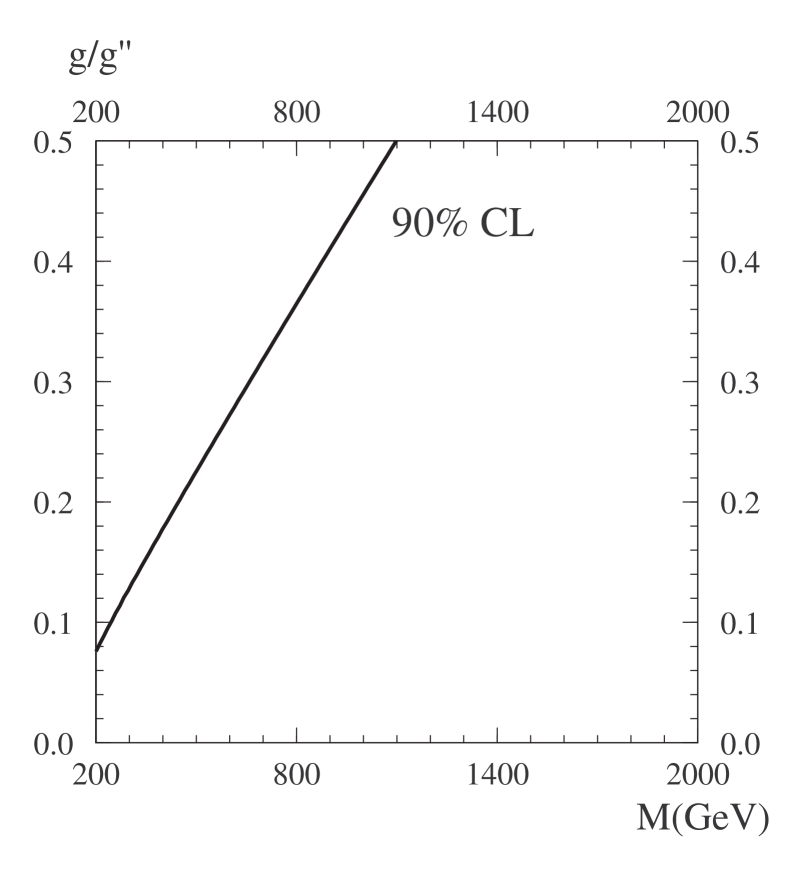
Figure 9: The bound in the $(M,g/g^{\prime\prime})$ parameter plane of the Degenerate BESS model arising from existing precision experimental data. The region to the left of the solid line is disallowed at $\geq 90\%$ CL.

Degenerate BESS - The Degenerate BESS model [7] describes two isotriplets of nearly degenerate vector resonances $(\vec{L},\vec{R})$ characterized by two parameters $(M,g^{\prime\prime})$, the common mass (when the EW interactions are turned off) and their gauge coupling. The main feature of the model is the decoupling property, which implies very loose bounds from existing precision experiments [13] as shown in Fig. 9. Another consequence is that the decay of the resonances into pairs of ordinary gauge vector bosons is quite depressed. The total widths for the two neutral states $(L_{3},R_{3})$ are given by

$$\Gamma_{L_{3},R_{3}}=M\,h_{L_{3},R_{3}}(g/g^{\prime\prime})\,,$$ (30)

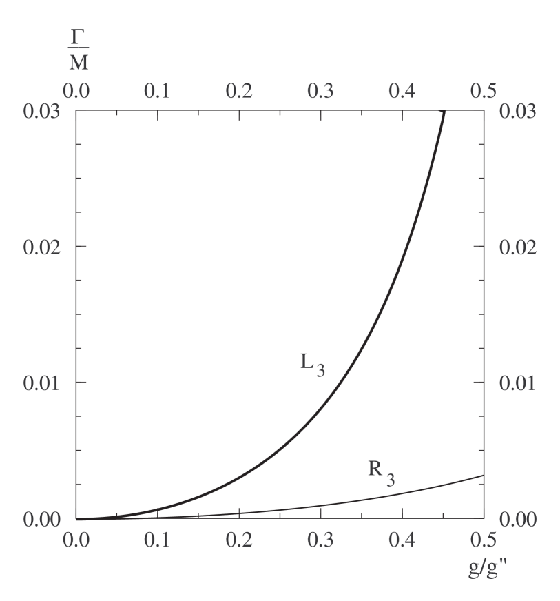
Figure 10: The ratio $\Gamma/M$ as a function of $g/g^{\prime\prime}$ for the Degenerate BESS for the neutral vector resonances $L_{3}$ and $R_{3}$.

where $g$ is the weak coupling constant. The behaviour of the total widths as functions of $g/g^{\prime\prime}$ is shown in Fig. 10, whereas for $g/g^{\prime\prime}\ll 1$ one has

$$h_{L_{3}}\approx 0.068\left(\frac{g}{g^{\prime\prime}}\right)^{2},~{}~{}~{}h_{R_{3}}\approx 0.01\left(\frac{g}{g^{\prime\prime}}\right)^{2}\,.$$ (31)

The ratio of the widths, $\Gamma_{L_{3}}/\Gamma_{R_{3}}$, in the interval $0\leq g/g^{\prime\prime}\leq.5$ approximately varies between $0.15$ and $0.07$. The weak interactions break the mass degeneracy giving rise to the mass splitting

$$M^{s}=M_{L_{3}}-M_{R_{3}}=M\,h_{M^{s}}(g/g^{\prime\prime})\,.$$ (32)

The behaviour of $h_{M^{s}}$ for $g/g^{\prime\prime}\ll 1$ is

$$h_{M^{s}}\approx(1-\tan^{2}\theta_{W})\left(\frac{g}{g^{\prime\prime}}\right)^{2}\approx 0.7\left(\frac{g}{g^{\prime\prime}}\right)^{2}\,.$$ (33)

The branching ratios into charged lepton pairs are almost parameter independent and rather sizeable

$$B(L_{3}\to\ell^{+}\ell^{-})\approx 4.5\%,~{}~{}~{}~{}B(R_{3}\to\ell^{+}\ell^{-})\approx 13.6\%\,.$$ (34)

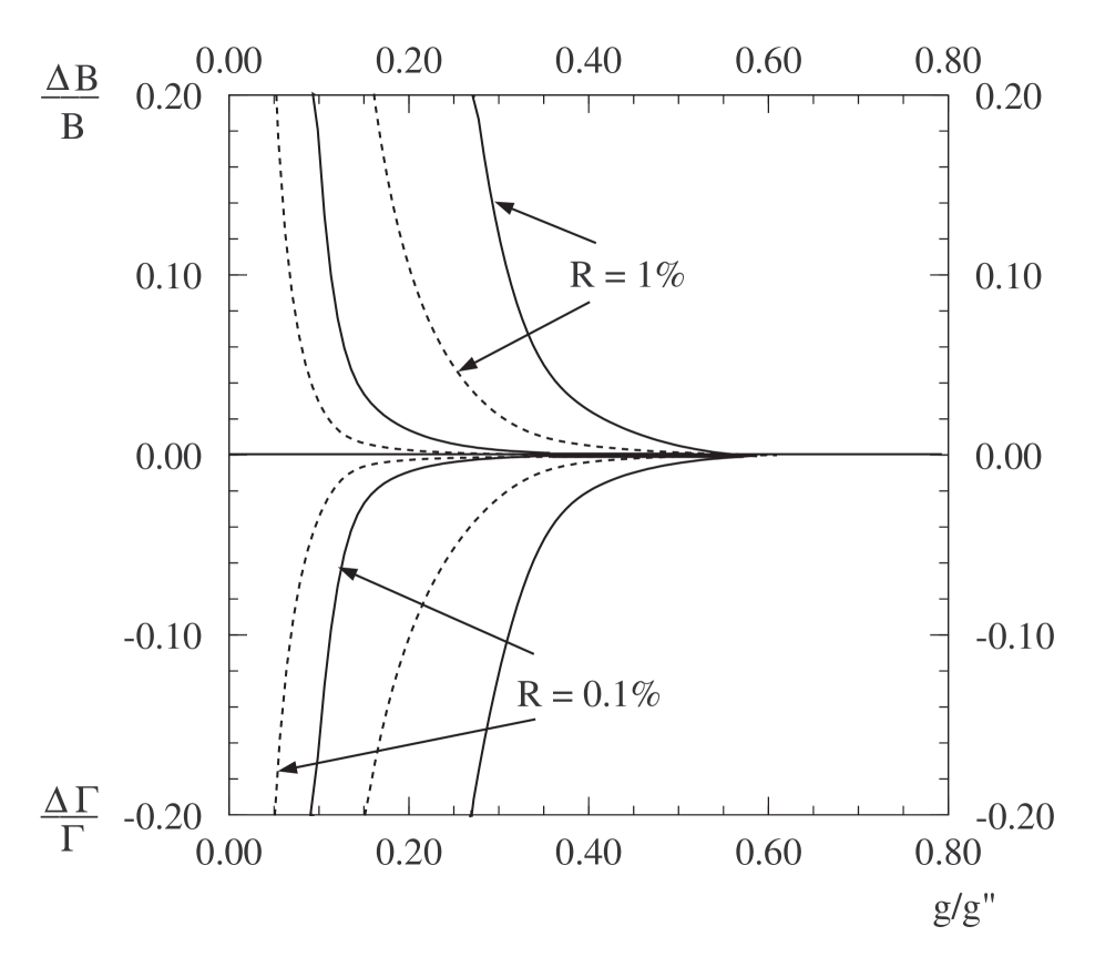
Figure 11: The Degenerate BESS model: the fractional errors on $B$ and $\Gamma$ for the vector resonance $L_{3}$ as functions of $g/g^{\prime\prime}$ from the three-point scan measurement ($E=M$, $E=M\pm 2\Gamma$), for $\Delta\sigma_{M}/\sigma_{M}=0.05$ (solid line) and $\Delta\sigma_{M}/\sigma_{M}=0.01$ (dashed line), and for $R=0.1\%$ and $R=1\%$.

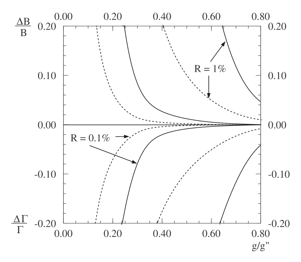
Figure 12: Same as in Fig. 11 for the vector resonance $R_{3}$.

In this Section, we will assume that $\sigma_{M}$ is much smaller than $M^{s}$, and therefore we can apply the previous analysis to the two resonances separately. The case $\sigma_{M}\approx M^{s}\gg\Gamma_{L_{3},R_{3}}$ will be studied in Section 4. By combining Fig. 2 with Fig. 10, we easily obtain the $\Delta\sigma_{M}$-induced fractional errors in the branching ratios and in the widths of the two resonances $L_{3}$ and $R_{3}$ as functions of $g/g^{\prime\prime}$ for different choices of $\sigma_{M}$ [equivalently, $R$; see Eq. (5)]. The results are given in Figs. 11 and 12 for $L_{3}$ and $R_{3}$, respectively, for the choices $\Delta\sigma_{M}/\sigma_{M}=1\%$ and 5%, and for $R=1\%$ and 0.1%. (Because the resonance widths are large, we do not need the very small values of $R$ required to study the SM Higgs or the $P^{0}$.) Combining these results with the bounds on the portion of parameter space still allowed by precision experiments, one can put lower limits on the masses of the resonances such that they have not been excluded and yet one is able to measure the widths with no more than a given systematic uncertainty from $\Delta\sigma_{M}$. For instance, in the case of a machine with $R=1\%$ (typical of an $e^{+}e^{-}$ collider) and for $\Delta\sigma_{M}/\sigma_{M}=1\%$, one finds, from Fig. 10, that $g/g^{\prime\prime}\mathrel{\raise 1.29167pt\hbox{$>$\kern-7.5pt\lower 4.30554pt\hbox{$\sim$}}}0.3$ is needed to avoid $\Delta\sigma_{M}$-induced errors in $\Gamma_{L_{3}}$ above $2\%$. From Fig. 9, the portion of parameter space that is still allowed by precision experiment can be roughly expressed by

$$\frac{M}{1000~{}{\rm GeV}}\mathrel{\raise 1.29167pt\hbox{$>$\kern-7.5pt\lower 4.30554pt\hbox{$\sim$}}}2.17\left(\frac{g}{g^{\prime\prime}}+0.01\right)\,.$$ (35)

Therefore, the $g/g^{\prime\prime}\mathrel{\raise 1.29167pt\hbox{$>$\kern-7.5pt\lower 4.30554pt\hbox{$\sim$}}}0.3$ requirement converts to the requirement that $M\mathrel{\raise 1.29167pt\hbox{$>$\kern-7.5pt\lower 4.30554pt\hbox{$\sim$}}}670~{}{\rm GeV}$. This means that, at lepton colliders with $R=1\%$ and $\Delta\sigma_{M}/\sigma_{M}=1\%$, one will be able to measure $\Gamma_{L_{3}}$ (for an allowed $L_{3}$ resonance) with a $\Delta\sigma_{M}$-induced error of less than 2% only if the mass of the resonance is greater than 670 GeV. Similar considerations apply to $R_{3}$, where keeping the systematic error in $\Gamma_{R_{3}}$ below $2\%$ requires $g/g^{\prime\prime}\mathrel{\raise 1.29167pt\hbox{$>$\kern-7.5pt\lower 4.30554pt\hbox{$\sim$}}}0.7$, leading to $M\mathrel{\raise 1.29167pt\hbox{$>$\kern-7.5pt\lower 4.30554pt\hbox{$\sim$}}}1540$ GeV. In the case of a muon collider, $R=0.1\%$ can be achieved while maintaining large luminosity. In this case, the $\Delta\sigma_{M}$-induced fractional error for $L_{3}$ is below $2\%$, for $\Delta\sigma_{M}/\sigma_{M}=1\%$, if $g/g^{\prime\prime}\mathrel{\raise 1.29167pt\hbox{$>$\kern-7.5pt\lower 4.30554pt\hbox{$\sim$}}}0.12$, which converts to $M\mathrel{\raise 1.29167pt\hbox{$>$\kern-7.5pt\lower 4.30554pt\hbox{$\sim$}}}280~{}{\rm GeV}$ for $L_{3}$ resonances not already excluded by the precision data. The corresponding limits for $R_{3}$ are $g/g^{\prime\prime}\mathrel{\raise 1.29167pt\hbox{$>$\kern-7.5pt\lower 4.30554pt\hbox{$\sim$}}}0.3$ and $M\mathrel{\raise 1.29167pt\hbox{$>$\kern-7.5pt\lower 4.30554pt\hbox{$\sim$}}}670~{}{\rm GeV}$. In particular, we see from Fig. 9 that, at a machine working at the top threshold (about 350 GeV), only resonances with $g/g^{\prime\prime}\mathrel{\raise 1.29167pt\hbox{$<$\kern-7.5pt\lower 4.30554pt\hbox{$\sim$}}}0.14$ have not already been excluded by the precision data. Therefore, only a machine with $R\leq 0.1\%$ would be able to measure the width and branching ratios of an allowed resonance without encountering significant systematic uncertainty coming from $\Delta\sigma_{M}/\sigma_{M}\sim 0.01$.

4 Analysis for nearly degenerate resonances

In this Section we will discuss nearly degenerate resonances, i.e. the case of a mass splitting much smaller than the average mass of the resonances, $M^{s}=M_{2}-M_{1}\ll M=(M_{1}+M_{2})/2$. We will be interested in the case where the energy spread of the beam is of the same order of magnitude as the mass splitting between the two peaks, $\sigma_{M}\approx M^{s}$. We will also assume that the widths of the two resonances are much smaller than the mass splitting, i.e. $\Gamma_{1},\,\Gamma_{2}\ll M^{s}$. It follows also that $\Gamma_{1},\,\Gamma_{2}\ll\sigma_{M}$. In this approximation, we can safely describe the cross section as the sum of two Breit-Wigner functions, and furthermore we can use the narrow width approximation. Therefore, 

$$M^{2}\sigma_{c}=B_{\ell^{+}\ell^{-}}^{1}\Phi(x_{1},\gamma_{1})+B_{\ell^{+}\ell^{-}}^{2}\Phi(x_{2},\gamma_{2})\,,$$ (36)

where $B_{\ell^{+}\ell^{-}}^{1}$ and $B_{\ell^{+}\ell^{-}}^{2}$ are the branching ratios of the resonances into $\ell^{+}\ell^{-}$, and

$$x_{1}=\frac{E-M_{1}}{\sigma_{M}},~{}~{}~{}x_{2}=\frac{E-M_{1}-M^{s}}{\sigma_{M}}=x_{1}-m^{s}$$ (37)

and

$$M_{2}=M_{1}+M^{s},~{}~{}~{}m^{s}=\frac{M^{s}}{\sigma_{M}}\,.$$ (38)

We have also assumed $M\approx M_{1}\approx M_{2}$. For a Gaussian beam we recall that the function $\Phi(x,\gamma)$ defined in Eq. (LABEL:scaled-conv) is given by

$$\Phi(x,\gamma)=\sqrt{\frac{\pi}{2}}(2j+1)\int_{-\infty}^{+\infty}e^{-(x-y)^{2}/2}\frac{\gamma^{2}}{y^{2}+\gamma^{2}/4}dy\,.$$ (39)

We may evaluate this expression by performing the Fourier transforms of the Gaussian distribution and of the Breit-Wigner and then taking the inverse Fourier transform. We get

$$\Phi(x,\gamma)=(2j+1)\pi^{3/2}\gamma\int_{-\infty}^{+\infty}dpe^{-p^{2}/2+ipx}\left(\theta(p)e^{-p\gamma/2}+\theta(-p)e^{+p\gamma/2}\right)\,.$$ (40)

Since we are assuming that the resonance widths are much smaller than the energy spread, we may evaluate Eq. (40) in the $\gamma\to 0$ approximation, yielding

$$\Phi(x,\gamma)=(2j+1)\gamma\sqrt{2}\pi^{3/2}e^{-x^{2}/2}\,,$$ (41)

as earlier given in Eq. (17) for $j=0$. As previously noted, this expression shows that when the energy spread is much bigger than the width the convolution gives rise to a Gaussian function with spread $\sigma_{M}$, and we loose any information about the total width. In fact, the total cross section $\sigma_{c}$ depends only on the product $B_{\ell^{+}\ell^{-}}\gamma=\Gamma(R\to\ell^{+}\ell^{-})/\sigma_{M}$. In the case of two resonances with $\gamma_{1},\,\gamma_{2}\to 0$, we thus find

$$M^{2}\sigma_{c}=(2j+1)\sqrt{2}\pi^{3/2}\left(g_{1}e^{-x_{1}^{2}/2}+g_{2}e^{-(x_{1}-m^{s})^{2}/2}\right)\,,$$ (42)

where

$$g_{i}=\gamma_{i}B^{i}_{\ell^{+}\ell^{-}}=\frac{\Gamma(R_{i}\to\ell^{+}\ell^{-})}{\sigma_{M}}\,.$$ (43)

The function (42) is invariant under the substitution

$$g_{1}\leftrightarrow g_{2},~{}~{}~{}x_{1}\leftrightarrow m^{s}-x_{1}$$ (44)

The behaviour of the function is characterized by the ratio

$$\frac{g_{2}}{g_{1}}=\frac{\Gamma(R_{2}\to\ell^{+}\ell^{-})}{\Gamma(R_{1}\to\ell^{+}\ell^{-})}\equiv a$$ (45)

and by $m^{s}$. For small $m^{s}$, the convolution of the Gaussian with the two Breit-Wigners has a single maximum in between 0 and $m^{s}$ depending on the value of $a$. For instance, for $a=1$ the maximum is at $m^{s}/2$. In this situation, the second derivative of the function (42) has two zeros corresponding to the changes of curvature before and after the peak. By increasing $m^{s}$ the second derivative acquires a third zero (in fact, a double zero). This is due to the effect of the smaller Breit-Wigner which gives rise to a further change of the curvature. Just to get an idea, we list in Table 5, for several choices of $a$, the critical value $m^{s}_{1}$ of $m^{s}$ at which this third zero occurs. As $m^{s}$ is increased further, there comes a point at which the two Breit-Wigner maxima start to show up. The minimum value of $m^{s}$ required to see two maxima, $m^{s}_{2}$, is given as a function of the ratio $a$ in Table 8. Notice that the invariance (44) implies $m^{s}_{i}(a)=m^{s}_{i}(1/a)$.

Table 8: Values of $m^{s}$ at which the double zero of the second derivative of the function (42) occurs ($m^{s}_{1}(a)$) and at which the two maxima of the function (42) start to show up ($m^{s}_{2}(a)$).

$a$	$m^{s}_{1}(a)$	$m^{s}_{2}(a)$
1	2	2
2	1.85	2.63
3	2.02	2.85
4	2.20	2.98
5	2.31	3.08

We can now discuss the type of measurements necessary to determine the parameters $M_{1}$, $M_{2}$, $g_{1}$ and $g_{2}$. In this discussion, we will use the notation $x\equiv x_{1}$. We first determine the overall location in energy of the resonance structure by locating the absolute maximum of the cross section. For small $m^{s}$, such that the individual resonance peaks are unresolved, the cross section has a single maximum near the location of the resonance with the larger $g$; we will assume that it is $g_{2}$ which is largest. For $m^{s}$ large enough that the peaks are resolved, we may locate the larger maximum. We denote the location of the maximum in the cross section by $E_{\rm max}$, and choose this as our first energy setting. We write

$$E_{\rm max}=\sigma_{M}x_{\rm max}+M_{1}\,,$$ (46)

where $x_{\rm max}$ is a function of $a$ and $m^{s}$ which can be evaluated numerically from Eq. (42). For instance, for $a\mathrel{\raise 1.29167pt\hbox{$>$\kern-7.5pt\lower 4.30554pt\hbox{$\sim$}}}2$ it is a good approximation to assume $x_{\rm max}\approx m^{s}$ (specially for $m^{s}$ bigger than the critical value $m^{s}_{2}$), implying $E_{\rm max}\simeq M_{2}$. The value of the cross section at $x_{\rm max}$ provides a second input into determining $M_{1,2}$ and $g_{1,2}$. To complete the process of determining these four parameters, we need two more measurements. If $m^{s}$ is larger than $m_{2}^{s}$, so that a second (lower) maximum is present, we can use the location of the second maximum and the cross section value at this second maximum as our two additional measurements. We effectively have four equations in four unknowns, two equations involving the derivatives of Eq. (42) and two involving the absolute magnitude of Eq. (42). If no second maximum is present, then we must effectively determine the slope of $\sigma_{c}(x)$ of Eq. (42) at some energy location away from $x_{\rm max}$ and determine the cross section at this same location. Measurements of $\sigma_{c}(x)$ at two nearby values of $x$ away from $x_{\rm max}$ are needed. That these approaches are really equivalent becomes apparent when we realize that the $m^{s}>m_{2}^{s}$ procedure of locating the second maximum actually requires measuring the slope of $\sigma_{c}(x)$ and finding its second zero. (Recall that this discussion assumes infinite statistics so that we will end up effectively computing the minimum error that will be induced by uncertainty in $\sigma_{M}$.)

In the absence of a second maximum, the choice of the other two energies can be difficult if $m^{s}$ is smaller than the critical value $m^{s}_{1}$. In fact, in this case the convolution of the two Breit-Wigner looks very much like the convolution with a single Breit-Wigner. Not surprisingly, to obtain reasonable errors it is necessary that $\sigma_{M}$ be such that $m^{s}$ is at least bigger than $m^{s}_{1}$. Let us assume that for $m^{s}>m^{s}_{1}$ we can approximately locate the energy corresponding to $x\sim 0$ and that we measure the cross section at two points in its vicinity (as well as at $x=x_{\rm max}$). If $m^{s}$ is greater than $m^{s}_{2}$, we may continue to employ the above procedure or we may use the alternative procedure outlined earlier based on the fact that the cross section has two maxima, one near $x=0$ and one near $x=m^{s}$; in the alternative procedure, we measure the energy and the cross section at the two peaks.

We consider first the former procedure that is the only choice if $m^{s}<m^{s}_{2}$. We start our analysis by taking $a=2$ and then later discuss the modifications for different values of $a$. From the measurement which fixes the energy scale (see Eq. (46)) we find the following relation between the parameter errors and the uncertainty in the energy spread:

$$\left(1+\frac{\Delta\sigma_{M}}{\sigma_{M}}\right)x_{\rm max}(m^{s}+\Delta m^{s})+\Delta m_{1}-x_{\max}(m^{s})=0\,,$$ (47)

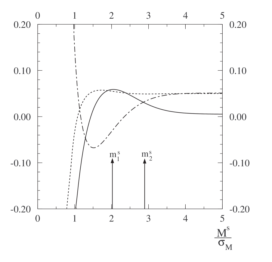
Figure 14: Same as in Fig. 13, with $a=3$.

where $\Delta M_{1}=\sigma_{M}\Delta m_{1}$ is the error in $M_{1}$ and $\Delta m^{s}$ is the error in $m^{s}$. From this equation we can eliminate $\Delta m_{1}$ in terms of the other errors. This has been done by using the approximation $x_{\rm max}\approx m^{s}$. The errors on $M^{s}$ and on the partial widths can then be determined using the three cross sections — $\sigma_{c}(x_{\rm max})$ and $\sigma_{c}(x)$ at two other $x$ values near 0 — following a procedure analogous to that discussed for a single resonance using Eq. (18). In particular, we assume measurements of the cross section at $x_{\max}$ and at $x=0.1$ and $x=0.2$. The resulting fractional errors for $\Gamma(R_{i}\to\ell^{+}\ell^{-})$ ($i=1,2$) and $M^{s}$ are given in Fig. 13 as a function of $M^{s}/\sigma_{M}$ for $\Delta\sigma_{M}/\sigma_{M}=5\%$. As expected, the errors grow rapidly once $m^{s}$ falls below $m^{s}_{1}$. As $m^{s}$ is increased above $m^{s}_{1}$, there is a change of curvature in the fractional error curves around the critical value $m^{s}_{2}$, after which the fractional errors approach asymptotic limits. Notice that the asymptotic value of $\Delta M^{s}/M^{s}$ is zero, whereas $\Delta\Gamma(R_{i}\to\ell^{+}\ell^{-})/\Gamma(R_{i}\to\ell^{+}\ell^{-})\to\Delta\sigma_{M}/\sigma_{M}$ for both $i=1,2$. This is because the cross sections depend only on the ratio $\Gamma(R_{i}\to\ell^{+}\ell^{-})/\sigma_{M}$. In Fig. 14 we represent the same quantities but for $a=3$, and we see results very similar to those for $a=2$ except for changes due to the different values of the critical points $m^{s}_{1}$ and $m^{s}_{2}$. We have tried different choices for the two measured points off the maximum, varying them up to $x=0.3$, without any significant change in the results.

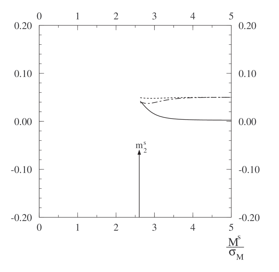
Figure 15: Same as in Fig. 13, again with $a=2$ but using the positions of the two maxima and the cross section values at the two maxima for determining the fractional errors.

We now consider the alternative procedure outlined earlier that is possible when two cross section maxima become visible, that is when the mass splitting is bigger than $m^{s}_{2}$. In this case, the four measurements for determining $M_{1,2}$ and $g_{1,2}$ are the energy locations of the two maxima and the cross sections at these two maxima. The measurement of the energy of the second maximum gives rise to a condition similar to the one of Eq. (47). The resulting fractional errors in $M^{s}$ and $\Gamma(R_{i}\to\ell^{+}\ell^{-})$ are given in Fig. 15 (for $a=2$), and are essentially the same as obtained in the previous procedure when $m^{s}>m^{s}_{2}$.

The basic conclusion from these analyses is that for $m^{s}$ of the order of the critical value $m^{s}_{2}$, the fractional errors in the parameters of the resonances are of the order of the fractional error in $\sigma_{M}$. For smaller $m^{s}$ the errors become very large. For $m^{s}$ significantly bigger than $m^{s}_{2}$, the fractional error in the mass splitting rapidly approaches zero while the fractional errors for the $\Gamma(R_{i}\to\ell^{+}\ell^{-})$ partial widths become equal to the fractional error in the energy spread. In short, we can use the critical value $m^{s}_{2}$ in order to discriminate between a good and a bad determination of the mass splitting.

5 Application to Degenerate BESS

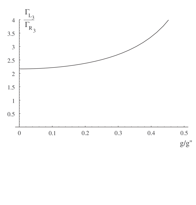
Figure 16: The ratio $\Gamma(L_{3}\to\ell^{+}\ell^{-})/\Gamma(R_{3}\to\ell^{+}\ell^{-})$ vs. $g/g^{\prime\prime}$ in the Degenerate BESS model.

In Degenerate BESS one can show that the condition $M^{s}\gg\Gamma_{L},\,\Gamma_{R}$ is rather well satisfied (by one and two orders of magnitude respectively). Therefore we can apply the analysis of the previous Section. From Fig. 16, we see that the value of $a$ is almost constant and approximately 2.2 for $g/g^{\prime\prime}$ up to 0.2, and then $a$ increases up to $\approx 4$ for $g/g^{\prime\prime}=0.5$. As discussed in the last Section, we can use the values of $m^{s}_{2}$ given in Table 8 in order to determine the minimum value of $M^{s}/\sigma_{M}$ needed in order to make a good determination of the mass splitting. For $a=2.2$ one finds that the minimum value is $m^{s}_{2}=2.68$. As in our earlier single resonance discussions, for any fixed value of the energy resolution $R$, we convert this bound into lower bounds for $g/g^{\prime\prime}$ and for the mass $M$ of nearly degenerate resonances that have not already been excluded by precision experimental data. From $M^{s}/\sigma_{M}\mathrel{\raise 1.29167pt\hbox{$>$\kern-7.5pt\lower 4.30554pt\hbox{$\sim$}}}2.68$ we get

We see that for $R=1\%$ a machine with energy near the top threshold would just be at the border of being able to accurately measure the mass difference between the $L_{3}$ and $R_{3}$ resonances not already excluded by precision data.

6 Conclusions

We have considered the production of a narrow resonance via $s$-channel collisions of leptons ($\ell=e$ or $\mu$). Here, a ‘narrow’ resonance is defined as one that has width $\Gamma$ substantially smaller than the beam energy spread $\Delta E_{\rm beam}$ that is natural for the collider (and therefore is associated with the largest instantaneous luminosity). It will be convenient to use the parameterization $\Delta E_{\rm beam}=0.01R\,E_{\rm beam}$, where $R$ is in per cent. For example, at a muon collider with center of mass energy $E\sim 100~{}{\rm GeV}$, $R\sim 0.12\%$ allows for maximal $L$ and $L$ declines rapidly as $R$ is forced to smaller values by compression techniques. A resonance with width $\Gamma\ll 0.001M$ would then be narrow. Our focus has been on the systematic error that might be introduced into measurements of the parameters of a narrow resonance due to systematic uncertainty in the value of $\Delta E_{\rm beam}/E_{\rm beam}$. The important parameters that can be measured are the branching ratio of the resonance into the charged leptons (i.e. those that are being collided), the product of this leptonic branching ratio times that for the resonance to decay to a particular final state, and the total width of the resonance. We examined four methods for determining the resonance parameters: (1) a scan of the resonance; (2) sitting on the resonance and changing the beam energy resolution; (3) measurement of the cross section in the $\ell^{+}\ell^{-}$ final state; and (4) measurement of the Breit-Wigner area. Methods (3) and (4) avoid the introduction of systematic errors due to uncertainty in $\Delta E_{\rm beam}/E_{\rm beam}$, but for the integrated luminosities that are anticipated to be available the statistical errors associated with these techniques would be quite large for a narrow resonance. Methods (1) and (2) can provide resonance parameter determinations with small statistical error. However, even in the limit of infinite statistical accuracy, determinations of the resonance parameters are sensitive to systematic uncertainties in $\Delta E_{\rm beam}$ if $\Gamma$ is not much larger than $\Delta E_{\rm beam}$. At a muon collider, the smallest $R$ that can be achieved is expected to be $R=0.003\%$, for which $\Delta E_{\rm beam}\sim\Gamma_{H}$ for a light SM Higgs boson and $\Delta E_{\rm beam}\sim\Gamma_{P^{0}}/2$ for the lightest pseudo goldstone boson of a technicolor model. Consequently, in these and other similar cases, a detailed assessment of the systematic errors in resonance parameter determinations introduced by uncertainty in $\Delta E_{\rm beam}$ is very important.

We have performed a general analysis to determine the (systematic) errors in the measured resonance parameters induced by a systematic uncertainty in $\Delta E_{\rm beam}$. We find that the induced fractional errors in the leptonic branching ratio (and also the product of the leptonic branching ratio times the branching ratio into any given final state) and in the total width can be expressed as universal functions of the ratio $\Gamma/\sigma_{M}$, where $\sigma_{M}$ is the spread in total center of mass energy resulting from the beam energy spreads: $\sigma_{M}/M=0.01R/\sqrt{2}$. In the case of the minimal three-point scan, with sampling at $E=M,E=M\pm k\Gamma$, the error functions also depend on $k$.

For a minimal three-point scan with $k=1$, the induced $\Delta\Gamma/\Gamma$ fractional systematic errors were parameterized as a function of $\Gamma/\sigma_{M}$ in Eq. (22). Very roughly, for $\Gamma/\sigma_{M}\sim 2.5$ we find that the induced fractional errors in $\Gamma$ and $B=B_{\ell^{+}\ell^{-}}$ or $B_{\ell^{+}\ell^{-}}B_{F}$ ($F$=final state) are of the order of the fractional uncertainty $\Delta\sigma_{M}/\sigma_{M}$. As $\Gamma/\sigma_{M}$ increases above 2, the fractional errors smoothly decrease. For values of $\Gamma/\sigma_{M}$ below 1, the fractional errors in the resonance parameters increase very rapidly. For example, for $\Gamma/\sigma_{M}\sim 1$ ($\sim 0.2$) the $\Delta\sigma_{M}$-induced fractional systematic errors in the resonance parameters increase to $\sim 3.5\div 4\Delta\sigma_{M}/\sigma_{M}$ ($\sim 20\div 25\Delta\sigma_{M}/\sigma_{M}$), for the $k=1$ scan. Thus, to avoid large systematic errors from $\Delta\sigma_{M}$, it is imperative to operate the collider with $\Gamma/\sigma_{M}$ no smaller than 1. If $R$ can be adjusted to achieve values significantly larger than 1, one can consider how to optimize the choice of $R$ so as to minimize the total statistical plus systematic error. A discussion was presented leading to the following two basic conclusions. (a) For a broad resonance, defined as one with $\Gamma\gg 0.001M$, one should operate the muon collider at its natural $R$ value of order $0.12\%$. The $\Delta\sigma_{M}$-induced errors will be very tiny, both because $\Gamma/\sigma_{M}$ is very large and because $\Delta\sigma_{M}/\sigma_{M}$ should be small for such $R$. (b) For a resonance with $\Gamma<0.001M$, one will typically wish to operate at an $R$ that is significantly smaller than that value which would yield equal statistical and systematic errors. In a typical case, this would mean a value of $R$ such that $\Gamma/\sigma_{M}$ is larger than $5\div 10$. Of course, if the resonance is extremely narrow, it may happen that $\Gamma/\sigma_{M}$ is of order, or not much larger than, unity even for $R=0.003\%$. In this case, it will normally be essential to run with $R=0.003\%$ even though this $R$ yields the smallest machine luminosity. Larger values of $R$ lead to a drastic decline in the signal to background ratio in a typical final state that, in turn, leads to very poor statistical errors (given the rather slow compensating increase with $R$ of the instantaneous luminosity).

For a narrow resonance with $\Gamma\ll 0.001M$, the technique in which one sits on the resonance peak and measures the cross section for two different values of $\sigma_{M}$ ($\sigma_{M}^{\rm max}>\Gamma$ and $\sigma_{M}^{\rm min}<\Gamma$) is a strong competitor to the scan technique. $\Gamma/\sigma_{M}^{\rm central}$ (where $\sigma_{M}^{\rm central}=\sqrt{\sigma_{M}^{\rm max}\sigma_{M}^{\rm min}}$) is determined by the ratio $r_{c}=\sigma_{c}(\sigma_{M}^{\rm min})/\sigma_{c}(\sigma_{M}^{\rm max})$, where $\sigma_{c}$ is the measured cross section. For $\sigma_{M}^{\rm max}/\sigma_{M}^{\rm min}$ of order 5 to 20, the statistical error in $\Gamma/\sigma_{M}^{\rm central}$ is smallest if $\Gamma/\sigma_{M}^{\rm central}\sim 2\div 3$. The larger $\sigma_{M}^{\rm max}/\sigma_{M}^{\rm min}$, the smaller the statistical error for $\Gamma/\sigma_{M}^{\rm central}$. For a typical choice of $\sigma_{M}^{\rm max}/\sigma_{M}^{\rm min}=10$, one finds a statistical error of $\Delta\Gamma/\Gamma\sim 1.8\Delta r_{c}/r_{c}$ for $\Gamma/\sigma_{M}^{\rm central}\sim 2\div 3$. This technique has the advantage that the $\Delta\sigma_{M}$-induced systematic error in $\Gamma$ is simply given by $\Delta\Gamma/\Gamma=\Delta\sigma_{M}/\sigma_{M}$, while there is no systematic error in the determination of any of the $B\equiv B_{\mu^{+}\mu^{-}}B_{F}$ branching ratio products ($F$ = a particular final state). Of course, if the resonance is very narrow (e.g. as narrow as a light SM Higgs boson or a light pseudogoldstone boson), $\Gamma/\sigma_{M}^{\rm central}\sim 2\div 3$ will not be achievable. In this case, the best that one can do is to employ $\sigma_{M}^{\rm min}$ ($\sigma_{M}^{\rm max}$) as given by $R=0.003\%$ ($R=0.03\%$). The statistical error in $\Gamma$ for such a situation is typically still very good.

Let us now summarize how these results apply in the specific cases we explored.

In the case of a three-point scan of the SM Higgs boson, we have shown that in the region $M_{H}\mathrel{\raise 1.29167pt\hbox{$<$\kern-7.5pt\lower 4.30554pt\hbox{$\sim$}}}110~{}{\rm GeV}$ it is mandatory to have $R\mathrel{\raise 1.29167pt\hbox{$<$\kern-7.5pt\lower 4.30554pt\hbox{$\sim$}}}0.003\%$. In fact, even for this very small $R$ value, $\Gamma_{H}/\sigma_{M}$ is still $\mathrel{\raise 1.29167pt\hbox{$<$\kern-7.5pt\lower 4.30554pt\hbox{$\sim$}}}1$, the very minimum needed for accurate measurements of resonance parameters. For $\Gamma_{H}/\sigma_{M}\sim 1$ the fractional systematic errors induced in $\Gamma_{H}$ from uncertainty in the beam energy spread are of order $3\Delta\sigma_{M}/\sigma_{M}$ for a $k=2$ scan. This should be compared to the typically-expected statistical errors tabulated in Table 5. For example, for $M_{H}=110~{}{\rm GeV}$ the statistical error in $\Delta\Gamma_{H}/\Gamma_{H}$ is $\sim 5\%$ for optimistic 4-year integrated luminosity of $L=4~{}{\rm fb}^{-1}$ at $R=0.003\%$; $\Delta\sigma_{M}/\sigma_{M}\mathrel{\raise 1.29167pt\hbox{$<$\kern-7.5pt\lower 4.30554pt\hbox{$\sim$}}}0.01$ would be needed for the systematic error to be smaller than the statistical error. For the pessimistic 4-year integrated luminosity of $L=0.4~{}{\rm fb}^{-1}$, the statistical error would be much larger (e.g. $\Delta\Gamma_{H}/\Gamma_{H}\sim 16\%$ at $M_{H}=110~{}{\rm GeV}$) and the $\Delta\sigma_{M}$-induced error would be much smaller than the statistical error if $\Delta\sigma_{M}/\sigma_{M}\mathrel{\raise 1.29167pt\hbox{$<$\kern-7.5pt\lower 4.30554pt\hbox{$\sim$}}}0.01$. Note, however, that increasing $R$ is not appropriate as this would push one into the $\Gamma_{H}/\sigma_{M}<1$ region, implying large statistical errors and still larger systematic errors.

For the $\sigma_{M}^{\rm max,min}$ on-peak ratio technique, one must choose $\sigma_{M}^{\rm min}$ corresponding to $R=0.003\%$ ($\Gamma_{H}/\sigma_{M}^{\rm min}\sim 1$). Results for statistical errors were presented in Table 6. As a point of comparison, for optimistic (pessimistic) instantaneous luminosity and 4 years of operation, the net production rate error after summing over important channels is of order 0.8% (2.7%) for $M_{H}=110~{}{\rm GeV}$, and the $\Delta\Gamma_{H}/\Gamma_{H}$ statistical error is of order 8% (25%). Although the statistical $\Delta\sigma_{c}/\sigma_{c}$ fractional error is somewhat smaller for the ratio technique than for the scan technique, the $\Delta\Gamma_{H}/\Gamma_{H}$ statistical error is larger. However, the ratio technique might still be better if $\Delta\sigma_{M}/\sigma_{M}$ were as large as $5\%$, especially if the optimistic luminosity level is available. This is because the systematic error in $\Gamma_{H}$ is equal to $\Delta\sigma_{M}/\sigma_{M}$ for the ratio technique as opposed to $3\Delta\sigma_{M}/\sigma_{M}$ for the scan technique. The $r_{c}$-ratio technique becomes increasingly superior as the assumed luminosity increases. For $M_{H}\geq 130~{}{\rm GeV}$, the ratio technique gives smaller statistical errors for both $\sigma_{c}B$ and $\Gamma_{H}$ than does the scan technique (for which statistical errors rapidly become very large). Indeed, the two procedures are nicely complementary in that at least one of them will allow a measurement of $\Gamma_{H}$ with statistical accuracy below 6% (20%) for optimistic (pessimistic) luminosity.

For the lightest PNGB ($P^{0}$) of an extended technicolor model, the $\Delta\sigma_{M}$-induced errors for the three-point scan method can be kept smaller than in the case of the SM Higgs boson. This is because, for typical model parameters, the $P^{0}$ has a width that is larger than that of a SM Higgs boson; $\Gamma_{P^{0}}/\sigma_{M}>2$ is quite likely for $R\approx 0.003\%$. For example, the parameter choices of [14] give $\Gamma_{P^{0}}\sim 5~{}{\rm MeV}$ vs. $\sigma_{M}\sim 2~{}{\rm MeV}$ at $M_{P^{0}}=100~{}{\rm GeV}$. As we have seen, the resulting $\Gamma_{P^{0}}/\sigma_{M}\sim 2.5$ yields $\Delta\sigma_{M}$-induced resonance parameter fractional errors of order $\Delta\sigma_{M}/\sigma_{M}$. This can be compared to the statistical errors given in Table 7, computed assuming the pessimistic 4-year integrated luminosity of $L=0.4~{}{\rm fb}^{-1}$. For example, at $M_{P^{0}}=110~{}{\rm GeV}$ the fractional statistical error for $\Gamma_{P^{0}}$ would be $\sim 0.04$, which is much larger than the systematic error if $\Delta\sigma_{M}/\sigma_{M}\sim 0.01$. For $M_{P^{0}}<80~{}{\rm GeV}$, the statistical error in $\Gamma_{P^{0}}$ declines to the $1\%\div 3\%$ level while the systematic error for $\Delta\sigma_{M}/\sigma_{M}=0.01$ rises to about this same level. As $M_{P^{0}}$ increases from $150~{}{\rm GeV}$ to $200~{}{\rm GeV}$, the statistical error for $\Gamma_{P^{0}}$ rises from $\sim 5\%$ to $\sim 10\%$ while the systematic error is below $1\%$ if $\Delta\sigma_{M}/\sigma_{M}=0.01$. For optimistic integrated luminosity of $L=4~{}{\rm fb}^{-1}$, the statistical errors would be smaller than quoted above. For $\Delta\sigma_{M}/\sigma_{M}=0.01$, the induced systematic errors would generally dominate for $M_{P^{0}}\leq 80~{}{\rm GeV}$.

The $P^{0}$ resonance is sufficiently narrow that one should also consider using the $\sigma_{M}^{\rm max,min}$ on-peak ratio technique to determine $\Gamma_{P^{0}}$. For 4-year pessimistic luminosity operation we find the statistical errors for $\Gamma_{P^{0}}$ given in Table 7. For the on-peak ratio technique, the systematic error in $\Gamma_{P^{0}}$ is equal to $\Delta\sigma_{M}/\sigma_{M}$ and for lower $M_{P^{0}}$ values would only be smaller than the statistical $\Gamma_{P^{0}}$ error if $\Delta\sigma_{M}/\sigma_{M}\mathrel{\raise 1.29167pt\hbox{$<$\kern-7.5pt\lower 4.30554pt\hbox{$\sim$}}}0.01$. For optimistic luminosity, the $1\%$ systematic error induced in $\Gamma_{P^{0}}$ for $\Delta\sigma_{M}/\sigma_{M}=0.01$ would dominate over the statistical error for all but $M_{P^{0}}\sim M_{Z}$ and $M_{P^{0}}>150~{}{\rm GeV}$. Most importantly, the statistical and systematic errors of the ratio technique are at least as good as, and often better than, obtained using the scan technique. For $M_{P^{0}}\leq 110~{}{\rm GeV}$, the statistical $\Gamma_{P^{0}}$ errors of the ratio technique are almost the same as obtained via the three-point scan (performed with $R=0.003\%$), while the systemic $\Gamma_{P^{0}}$ errors from the ratio technique are smaller ($\Delta\sigma_{M}/\sigma_{M}$ vs. $\sim 1.5\Delta\sigma_{M}/\sigma_{M}$). For $M_{P^{0}}\geq 120~{}{\rm GeV}$, the $\Delta\sigma_{M}$-induced systematic errors are comparable for the two techniques, but the statistical errors for the ratio technique are substantially smaller than for the three-point scan. Precision measurements of the properties of a $P^{0}$ resonance would, thus, always be best performed using the ratio procedure.

In the case of the two resonances of the Degenerate BESS model, we have determined (for several typical $R$ values) the region of the model parameter space for which the fractional errors in the resonance properties ($\Gamma$, $\ldots$) induced by $\Delta\sigma_{M}$ are less than a given fixed value. Induced errors are small for large resonance masses. But, for any given choice of $R$, as the resonance mass is decreased, while maintaining model parameter choices such that the model is still consistent with precision experimental data, there comes a point at which, even for $\Delta\sigma_{M}/\sigma_{M}\sim 0.01$, the induced error becomes large. For allowed model parameter choices yielding a resonance mass below this, the resonance’s properties cannot be measured accurately. The lowest masses of the resonances that correspond to precision-data-allowed BESS model parameters, and for which $\Delta\sigma_{M}$-induced errors in the measured resonance properties are small, decrease rapidly with decreasing $R$. As a result, the ability to achieve $R<0.1\%$ at a muon collider would be crucial for exploring the low-resonance-mass portions of Degenerate BESS parameter space not currently excluded by precision data.

Finally, we have performed the analysis of two nearly degenerate resonances, a situation encountered in a number of theoretical examples, including the Degenerate BESS model and the minimal supersymmetric model. We focused on the case in which the total widths of the resonances are much smaller than the mass splitting. We have shown that, in general, the $\Delta\sigma_{M}$-induced fractional error in the measured mass splitting, $M^{s}$, and in the leptonic partial widths of the resonances (or leptonic partial widths times final state branching fraction) depend only on $M^{s}/\sigma_{M}$ and on the ratio of the two partial widths, $a$. The main result is that the errors are generally big for $M^{s}/\sigma_{M}$ less than a certain critical value (typically in the $2\div 3$ range) that is a function of $a$. As $M^{s}/\sigma_{M}$ increases beyond the critical value, the $\Delta\sigma_{M}$-induced fractional error in the mass splitting approaches zero rapidly, whereas the fractional errors in the partial widths approach $\Delta\sigma_{M}/\sigma_{M}$. As a concrete case, we have discussed the application to the two spin-1 resonances of the Degenerate BESS model for beam energy spread of the same order as the mass splitting between them. We determined the regions of the model parameter space in which $M^{s}$ could be measured with $\Delta\sigma_{M}$-induced fractional error below a given fixed value assuming a given value of $R$. The smaller the value of $R$ that can be used while maintaining sufficient luminosity for small statistical errors, the larger the fraction of allowed parameter space for which $M^{s}$ can be measured with small $\Delta\sigma_{M}$-induced error. In particular, $R<0.1\%$ is required if we are to be able to separate the degenerate resonance peaks for model parameter choices not already excluded by precision experimental data in which the resonance masses are as low as $100~{}{\rm GeV}$.

Acknowledgements We wish to thank A. Blondel for the interesting discussions during the CERN Workshop on muon colliders, where this paper was conceived. JFG is supported in part by the U.S. Department of Energy and by the Davis Institute for High Energy Physics.

Figure 3: $\Gamma/\sigma_{M}^{\rm central}$ plotted as a function of the cross section ratio $\sigma_{c}(\sigma_{M}^{\rm min})/\sigma_{c}(\sigma_{M}^{\rm max})$ for various values of $\sigma_{M}^{\rm max}/\sigma_{M}^{\rm min}$ keeping $\sigma_{M}^{\rm central}\equiv\sqrt{\sigma_{M}^{\rm max}\sigma_{M}^{\rm min}}$ fixed.

References

- [1] The following web pages contain informations on muon collider studies: www.fnal.gov/projects/muoncollider; www.cap.bnl.gov/mumu/muhomepage.html; www.hep.princeton.edu/mumu/nice; www.cern.ch/autin/MuonsAtCERN/index.htm.
- [2] V. Barger, M.S. Berger, K. Fujii , J.F. Gunion, T. Han, C. Heusch, W. Hong, S.K. Oh, Z. Parsa, S. Rajpoot, R. Thun and B. Willis, Proceedings of the Workshop on Physics Potential and Development of Colliders, 2nd, Sausalito, CA, 17-19 Nov 1994, ed. D. B. Cline. Amer. Inst. Phys., p. 55 (1996). V. Barger, M.S. Berger, J.F. Gunion and T. Han, ITP Proceedings of the Conference on Future High Energy Colliders, Santa Barbara, CA, 21-25 Oct 1996, ed. Z. Parsa. Amer. Inst. Phys., p. 219 (1997). J.F. Gunion, Proceedings of the 5th International Conference on Physics Beyond the Standard Model, Balholm, Norway, April-May 1997, eds. G. Eigen, P. Osland and B. Stugu, Amer. Inst. Phys., p. 234 (1997). J.F. Gunion, Proceedings of the Workshop on Physics at the First Muon Collider and at the Front End of a Muon Collider, Batavia, IL, 6-9 Nov 1997, eds. S. Geer and R. Raja. Amer. Inst. Phys., p. 37 (1998). C. Quigg, Proceedings of the Workshop on Physics at the First Muon Collider and at the Front End of a Muon Collider, Batavia, IL, 6-9 Nov 1997, eds. S. Geer and R. Raja. Amer. Inst. Phys., p. 242 (1998). V. Barger, Proceedings of the International Conference on Physics Potential and Development of Colliders (MUMU 97), 4th, San Francisco, CA, 10-12 Dec 1997, ed. D.B. Cline, Amer. Inst. Phys. (1998).
- [3] V. Barger, M.S. Berger, J.F. Gunion, and T.Han, Phys. Rev. Lett. 75 (1995) 1462; ibidem, Phys. Rep. 286 (1997) 1.
- [4] R. Casalbuoni, S. De Curtis, A. Deandrea, D. Dominici, R. Gatto and J.F. Gunion, hep-ph/9904253, April, 1999.
- [5] J.F. Gunion, Proceedings of the 5th International Conference on Physics Beyond the Standard Model, Balholm, Norway, 29 Apr – 4 May 1997, eds. G. Eigen, P. Osland and B. Stugu, AIP (1997), p. 234.
- [6] M. Demarteau and T. Han, Proceedings of the Workshop on Physics at the First Muon Collider and at the Front End of a Muon Collider, Batavia, IL, 6-9 Nov 1997, eds. S. Geer and R. Raja. Amer. Inst. Phys., p. 177 (1998). V. Barger, Proceedings of the 5th International Conference on Supersymmetries in Physics (SUSY 97), Philadelphia, PA, May 1997, eds. M. Cvetic and P. Langacker. Amsterdam, North- Holland, 1998, Nucl. Phys. Proc. Suppl. 62, p. 13 (1998).
- [7] R. Casalbuoni, A. Deandrea, S. De Curtis, D. Dominici, F. Feruglio, R. Gatto, M. Grazzini, Phys. Lett. B349 (1995) 533. R. Casalbuoni, A. Deandrea, S. De Curtis, D. Dominici, R. Gatto, M. Grazzini, Phys. Rev. D53 (1996) 5201. R. Casalbuoni, S. De Curtis, D. Dominici, M. Grazzini, Phys. Rev. D56 (1997) 2812.
- [8] Proceedings of the DPF/DPB Summer Study on New Directions for High-Energy Physics (Snowmass 96), Snowmass, CO, 25 Jun - 12 Jul 1996, eds. D.G. Cassel, L. Trindle Gennari and R.H. Siemann, Stanford Linear Accelerator Center (1997) (C96/06/25).
- [9] R. Raja and A. Tollestrup, Proceedings of the Workshop on Physics at the First Muon Collider and at the Front End of a Muon Collider, Batavia, IL, 6-9 Nov 1997, eds. S. Geer and R. Raja. Amer. Inst. Phys., p. 583 (1998).
- [10] C.M. Ankenbrandt et al., [Muon Collider Collaboration], Status of Muon Collider Research and Development and Future Plans, FERMILAB-PUB-98-179, January, 1999.
- [11] B. Autin et al., Report of Prospective Study of Muon Storage Rings in Europe, to be published as a CERN yellow Report.
- [12] A. Djouadi, D. Haidt, B.A. Kniehl, B. Mele and P.M. Zerwas, Proceedings of the Workshop - Munich, Annecy Hamburg, February 4 to September 3, 1991, Part A, DESY 92-123A, ed. P.M. Zerwas, p. 11 (1992).
- [13] D. Karlen, Proceedings of the International Conference on High-energy Physics. 29th, (ICHEP 98), Vancouver, Canada, 23-29 Jul 1998.
- [14] R. Casalbuoni, S. De Curtis, A. Deandrea, D. Dominici, R. Gatto and J.F. Gunion, Proceedings of the Workshop on Physics at the First Muon Collider and at the Front End of a Muon Collider, Batavia, IL, 6-9 Nov 1997, eds. S. Geer and R. Raja. Amer. Inst. Phys., p. 772 (1998).; ibidem UCD-98-13, DFF-316-7-98, UGVA-DPT-07-1011, hep-ph/9809523 (to be published on Nucl. Phys.).
- [15] K. Lane, BUHEP-98-01, hep-ph/9801385. E. Eichten, K. Lane and J. Womersley, Phys. Rev. Lett. 80 (1998) 5489.
- [16] E. Fahri and L. Susskind, Phys. Rep. 74 (1981) 277.